On Tuning Parameter Selection in Model Selection and Model Averaging: A Monte Carlo Study

Abstract

Model selection and model averaging are popular approaches for handling modeling uncertainties. The existing literature offers a unified framework for variable selection via penalized likelihood and the tuning parameter selection is vital for consistent selection and optimal estimation. Few studies have explored the finite sample performances of the class of ordinary least squares (OLS) post-selection estimators with the tuning parameter determined by different selection approaches. We aim to supplement the literature by studying the class of OLS post-selection estimators. Inspired by the shrinkage averaging estimator (SAE) and the Mallows model averaging (MMA) estimator, we further propose a shrinkage MMA (SMMA) estimator for averaging high-dimensional sparse models. Our Monte Carlo design features an expanding sparse parameter space and further considers the effect of the effective sample size and the degree of model sparsity on the finite sample performances of estimators. We find that the OLS post-smoothly clipped absolute deviation (SCAD) estimator with the tuning parameter selected by the Bayesian information criterion (BIC) in finite sample outperforms most penalized estimators and that the SMMA performs better when averaging high-dimensional sparse models.

1. Introduction

Model selection and model averaging have long been the competing approaches in dealing with modeling uncertainties in practice. Model selection estimators help us search for the most relevant variables, especially when we suspect that the true model is likely to be sparse. On the other hand, model averaging aims to smooth over a set of candidate models so as to reduce risks relative to committing to a single model.

Uncovering the most relevant variables is one of the fundamental tasks of statistical learning, which is more difficult if modeling uncertainty is present. The class of penalized least squares estimators have been developed to handle modeling uncertainty. Fan and Li (2006) laid out a unified framework for variable selection via penalized likelihood.

Tuning parameter selection is vital in the optimization of the penalized least squares estimators for achieving consistent selection and optimal estimation. To select the proper tuning parameter, the existing literature offers two frequently applied approaches, which are the cross-validation (CV) approach and the information criterion (IC)-based approach. Shi and Tsai (2002) have shown that the Bayesian information criterion (BIC), under certain conditions, can consistently identify the true model when the number of parameters and the size of the true model are both finite. Wang et al. (2009) further proposed a modified BIC for tuning parameter selection when the number of parameters diverges with the increase in the sample size.

Although most of the penalized least squares estimators such as the adaptive least absolute shrinkage and selection operator (AdaLASSO) by Zou (2006), the smoothly clipped absolute deviation penalty (SCAD) estimator by Fan and Li (2001), and the minimax concave penalty (MCP) estimator by Zhang (2010) have been researched with well-documented finite sample performances, few studies have focused on the finite sample performances of the class of ordinary least squares (OLS) post-selection estimators with the tuning parameter choice determined by different tuning parameter selection approaches.

Despite decent selection performance from the current penalized least squares estimators, there is not yet a unified approach in estimating the distribution of such estimators, due to the complicated constraints and penalty functions. Knight and Fu (2000); Pötscher and Leeb (2009) and Pötscher and Schneider (2009) investigated the distributions of LASSO-type and SCAD estimators and concluded that they tend to be highly non-normal. Hansen (2014) stated that the distribution for model selection and model averaging estimators are highly non-normal but routinely ignored. This ushered in the development of the class of post-selection estimators such as the OLS post-LASSO estimator by Belloni and Chernozhukov (2013). Such a class of OLS post-selection estimators avoids the complicated constraints and penalty functions when building inferences.

Model averaging is applied to hedge against the risks stemming from the possible specification errors of a single model. For this paper, we attempt to combine the model selection and model averaging approaches to deal with modeling uncertainty. Therefore, inspired by the shrinkage averaging estimator (SAE) by Schomaker (2012) and the Mallows model averaging (MMA) criterion by Hansen (2007), we further propose a shrinkage Mallows model averaging (SMMA) estimator to reduce the asymptotic risks in high-dimensional sparse models from possible specification errors. Briefly, the existing model averaging methods lack a systematic rule in selecting candidate models, while penalty estimation methods are sensitive to the choice of tuning parameters. The shortcomings of these two methods motivate us to propose our SMMA estimator, which effectively combines these two methods to address such weaknesses. That is, our estimator provides a data-driven approach to select the candidate models for averaging, while at the same time, the usage of a set of data-driven tuning parameters relieves the sensitivity problem of the shrinkage estimators. Finite sample performances from the SMMA will be compared with some of the existing model averaging estimators.

The Monte Carlo design is similar to that of Wang et al. (2009), which features an expanding sparse parameter space as the sample size increases. Our Monte Carlo design further considers the effect of changes in the effective sample size and the degree of model sparsity on the finite sample performances of model selection and model averaging estimators. We find that the OLS post-SCAD(BIC) estimator in finite samples outperforms most of the current penalized least squares estimators. In addition, the SMMA performs better given sparser models. This supports the use of the SMMA estimator when averaging high dimensional sparse models.

The rest of the paper is organized as follows. Section 2 gives a brief review of the existing model selection and model averaging estimators in the literature. Section 3 introduces our proposed SMMA estimator. Section 4 reports the finite sample performances of the OLS post-selection estimators and compares the finite sample performance of the SMMA with those of the existing model averaging estimators. Section 5 concludes.

2. Literature Review

In this section, we will review some of the frequently applied model selection and model averaging estimators in the existing literature. We start by defining a simple linear model from which the corresponding model selection and model averaging estimators will be defined, respectively, in the following subsections. Consider a simple linear model given by

$$y_i=X_i^T\beta +{\epsilon }_i,\forall i=1,2,\cdots ,n,$$

(1)

where $X_i$ is a $p\times 1$ vector of exogenous regressors, and $\beta$ is a $p\times 1$ parameter vector with only $p_0$ number of nonzero parameters. We further assume that $p_0<p$ and that the error term ${\epsilon }_i\sim i.i.d(0,{\sigma }^2)$. The literature on model selection and model averaging is large and continues to grow with time. Our review below is limited to the most frequently used model selection and model averaging estimators.

2.1. Model Selection

The traditional best subsets approach predating the class of penalized least squares estimators is generally computationally costly and highly unstable due to the discrete nature of the selection algorithm, as pointed out in Fan and Li (2001). The subsequent stepwise approach, which is essentially a variation of the best subsets approach, frequently fails to generate a solution path that leads to the global minimum. In addition, both approaches assume all variables are relevant, even if the underlying true model might have a sparse representation. Then came the class of penalized least squares estimators, which minimize the loss function subjected to some forms of penalty. Some of the frequently applied penalized least squares estimators include the ridge estimator, the LASSO-type estimators, the SCAD estimator, and the MCP estimator.

Hoerl and Kennard (1970) introduced the original ridge estimator with an $l_2$ penalty. The ridge estimator is defined as

$${\widehat{\beta }}^{ridge}=\underset{\beta }{argmin}{∥y-X\beta ∥}^2+\lambda \sum _{k=1}^p{\beta }_k^2,$$

(2)

where $\lambda$ is the so-called tuning parameter.

Tibshirani (1996) introduced an $l_1$ -penalty and constructed the LASSO estimator as follows:

$${\widehat{\beta }}^{LASSO}=\underset{\beta }{argmin}{∥y-X\beta ∥}^2+\lambda \sum _{k=1}^p|{\beta }_k|.$$

(3)

Compared to the best subsets approach, where all possible subsets need to be evaluated for variable selection, both of the ridge and LASSO estimators conduct the selection and estimation of the parameters simultaneously, thus gaining computational savings. However, both estimators fail to satisfy the oracle properties, due to inconsistent selection and asymptotic bias. The oracle properties describe the ability of an estimator to perform the same asymptotically, as if we knew the true specification of the model beforehand. In the high-dimensional parametric estimation literature, an oracle efficient estimator is therefore able to simultaneously identify the nonzero parameters and achieve optimal estimation of the nonzero parameters. However, Fan and Li (2001) and Zou (2006), among others, questioned whether the LASSO satisfies the oracle properties.

Thus, various LASSO-type estimators have been developed since then to overcome the selection bias of the original ridge and LASSO estimator. Zou and Hastie (2005) introduced the elastic net estimator by averaging between the $l_1$ penalty and $l_2$ penalty. Specifically, the elastic net estimator is defined as

$${\widehat{\beta }}^{ElasticNet}=\underset{\beta }{argmin}{∥y-X\beta ∥}^2+{\lambda }_1\sum _{k=1}^p|{\beta }_k|+{\lambda }_2\sum _{k=1}^p{\beta }_k^2,$$

(4)

where depending on the choices of the two tuning parameters, ${\lambda }_1$ and ${\lambda }_2$, the elastic net estimator combines the properties of the ridge estimator and the LASSO estimator and enjoys the oracle properties.

Zou (2006) further introduced a LASSO-type estimator, namely the adaptive LASSO estimator, which is defined as

$${\widehat{\beta }}^{AdaLASSO}=\underset{\beta }{argmin}{∥y-X\beta ∥}^2+\lambda \sum _{k=1}^p{\widehat{w}}_k|{\beta }_k|,$$

(5)

where the adaptive weights ${\widehat{w}}_k={|{\widehat{\beta }}_k^{*}|}^{-\gamma }$ with $\gamma >0$, and ${\widehat{\beta }}^{*}$ denotes any root-n consistent estimator for $\beta$. The adaptive LASSO estimator also fulfills the oracle properties.

Fan and Li (2001) proposed the smoothly clipped absolute deviation (SCAD) penalty estimator, which features a symmetric non-concave penalty function that leads to sparse solutions. The SCAD estimator is defined as

$${\widehat{\beta }}^{SCAD}=\underset{\beta }{argmin}{∥y-X\beta ∥}^2+\sum _{k=1}^{p}F\left(\right|{\beta }_k|;\lambda ,\gamma ),$$

(6)

where the continuously differentiable penalty function $F\left(\right|\beta |;\lambda ,\gamma )$ is defined as

$$F\left(\right|\beta |;\lambda ,\gamma )=\left\{\begin{array}{cc}\lambda \left|\beta \right|\hfill & \mathrm{if}\left|\beta \right|\le \lambda \hfill \\ \frac{2\gamma \lambda \left|\beta \right|-{\left|\beta \right|}^2-{\lambda }^2}{2\gamma -1}\hfill & \mathrm{if}\gamma \lambda >\left|\beta \right|>\lambda \hfill \\ \frac{{\lambda }^2(\gamma +1)}{2}\hfill & \mathrm{if}\left|\beta \right|\ge \gamma \lambda \hfill \end{array}\right.,$$

(7)

and $\gamma$ defaults to $3.7$ following the recommendation from Fan and Li (2001).

Zhang (2010) introduced the minimax concave penalty (MCP) estimator, which produces nearly unbiased variable selection. The MCP estimator is defined as

$${\widehat{\beta }}^{MCP}=\underset{\beta }{argmin}{∥y-X\beta ∥}^2+\sum _{k=1}^{p}F\left(\right|{\beta }_k|;\lambda ,\gamma ),$$

(8)

where the continuously differentiable penalty function $F\left(\right|\beta |;\lambda ,\gamma )$ is defined as

$$F\left(\right|\beta |;\lambda ,\gamma )=\left\{\begin{array}{cc}\lambda \left|\beta \right|-\frac{{\left|\beta \right|}^2}{2\gamma },\hfill & \mathrm{if}\left|\beta \right|\le \lambda \gamma \hfill \\ \frac{1}{2}\gamma {\lambda }^2,\hfill & \mathrm{if}\left|\beta \right|>\lambda \gamma \hfill \end{array}\right.,$$

(9)

and $\gamma$ defaults to 3, as suggested by Breheny and Huang (2011).

2.1.1. Choice of Tuning Parameter

Tuning parameters play a crucial role in the optimization problem for the aforementioned penalized least squares estimators to achieve consistent selection and optimal estimation. There exists an extensive debate in the model selection literature regarding the proper choice for the tuning parameter. Two of the frequently applied approaches used to select the tuning parameter are the n-fold cross-validation (CV), or the generalized cross-validation (GCV) approach, and the information criterion (IC)-based approach. In practice, the CV approach could also be computationally costly for big datasets.

The traditional IC approaches have been modified for the selection of the tuning parameters in the penalized least squares framework. Shi and Tsai (2002) have shown that the BIC, under certain conditions, can consistently identify the true model when the number of parameters and the size of the true model are finite. For scenarios where the number of parameters diverges with the increase in the sample size, Wang et al. (2009) proposed a modified BIC for the selection of the tuning parameter. This criterion yields consistent selection and reduces asymptotic risks. Fan and Tang (2013) further introduced a generalized information criterion (GIC) for determining the optimal tuning parameters in penalty estimators. They proved that the tuning parameters selected by such a GIC produce consistent variable selection and generate computational savings.

Regarding the generation of the candidate tuning parameters in the penalized likelihood framework, Tibshirani et al. (2010) first introduced the cyclical coordinate descent algorithm to compute the solution path for generalized linear models with convex penalties such as LASSO and Elastic Net. This algorithm helps generate a set of candidate tuning parameters to facilitate the selection of the optimal tuning parameter. Breheny and Huang (2011) further applied this algorithm to calculate the solution path for non-convex penalty estimators such as the SCAD and MCP estimators. They compared the performances of some of the popular penalty estimators such as the LASSO, SCAD, and MCP estimators for variable selection in sparse models. Their simulation study and data examples indicated that the choice of the tuning parameter greatly affects the outcome of the variable selection.

2.1.2. Post-Selection Estimators

Despite decent selection performance from the current mainstream penalized least squares estimators, there is not yet a unified approach in estimating the distribution of such estimators, due to the complicated constraints and penalty functions. Knight and Fu (2000); Pötscher and Leeb (2009) and Pötscher and Schneider (2009), among others, investigated the distributions of LASSO-type and SCAD estimators and concluded that they tend to be highly non-normal. This ushered in the burgeoning development in post-model-selection inferential methods. Hansen (2014) stated that the distributions for the model selection and model averaging estimators are highly non-normal but routinely ignored in practice. Belloni and Chernozhukov (2013) proposed the OLS post-LASSO estimator, which, under certain assumptions, outperforms the LASSO estimator in reducing asymptotic risks associated with high-dimensional sparse models. The OLS post-LASSO estimator utilizes the LASSO estimator as a variable selection operator in the first step and reverts back to the OLS estimator to produce parameter estimates for the selected model in the second step. Such an estimator avoids the complicated penalty functions in estimating the distribution of the estimator in the second step and thus yields easier access to inference that is solely based on the OLS estimator. Inspired by the OLS post-LASSO estimator, other post-selection estimators could be constructed with the tuning parameters in the penalty function selected by either the BIC or GCV approach.

For example, an OLS post-SCAD(BIC) estimator can be constructed with the tuning parameter in the penalty function selected by the BIC approach. More specifically, let $\Lambda =\{{\lambda }^1,\cdots ,{\lambda }^q\}$ be the set of candidate tuning parameters and $|\Lambda |=q$ with $q\in {\mathbb{Z}}^{+}$ .

Given any $\lambda \in \Lambda$ and $\gamma$ defaulting to 3.7, the SCAD estimator from Equation (6) evaluated at $\lambda$ gives

$${\widehat{\beta }}^{\lambda }=\underset{\beta }{argmin}{∥y-X\beta ∥}^2+\sum _{k=1}^{p}F\left(\right|{\beta }_k|;\lambda ).$$

(10)

The BIC evaluated at this $\lambda$ is defined as $BI{C}_{\lambda }$, which is given by

$$BI{C}_{\lambda }=log\left(\frac{{∥y-X{\widehat{\beta }}^{\lambda }∥}^2}{n}\right)+\left|S_{\lambda }\right|\frac{log\left(n\right)}{n}{C}_n,$$

(11)

where the values for $\lambda$ originate from an exponentially decaying grid as in Tibshirani et al. (2010). Let $S_{\lambda }$ denote the set of nonzero parameters of the model when evaluated at $\lambda$, and more specifically, $S_{\lambda }=\{k:{\widehat{\beta }}_k^{\lambda }\ne 0\}$. For any set $\mathbb{S}$, let $\left|\mathbb{S}\right|$ represent its cardinality. Then, $|S_{\lambda }|$ gives the number of nonzero parameters of the model when evaluated at $\lambda$, and $C_n$ is a constant. Shi and Tsai (2002) have shown that the above BIC with $C_n=1$ consistently identifies the true model when both p and $p_0$ are finite.

The estimate of the optimal tuning parameter is denoted by ${\widehat{\lambda }}^{BIC}$, which is the solution to the following problem:

$${\widehat{\lambda }}^{BIC}=\underset{\lambda \in \{{\lambda }^1,\cdots ,{\lambda }^q\}}{argmin}BI{C}_{\lambda }.$$

(12)

Consequently, ${\widehat{\beta }}^{{\widehat{\lambda }}^{BIC}}$ minimizes the SCAD penalized objective function given by Equation (6); i.e.,

$${\widehat{\beta }}^{{\widehat{\lambda }}^{BIC}}=\underset{\beta }{argmin}{∥y-X\beta ∥}^2+\sum _{k=1}^{p}F(|{\beta }_k|,{\widehat{\lambda }}^{BIC}).$$

(13)

Denoting $S_{{\widehat{\lambda }}^{BIC}}=\{k:{\widehat{\beta }}_k^{{\widehat{\lambda }}^{BIC}}\ne 0\}$, we define the OLS post-SCAD(BIC) estimator as

$${\widehat{\beta }}^{BIC}=\underset{\beta }{argmin}{∥y-\sum _{l\in S_{{\widehat{\lambda }}^{BIC}}}^{}{X}_l{\beta }_l∥}^2,$$

(14)

where $X_l$ is an $n\times 1$ vector, which is the $l^{th}$ column of the predictor matrix X, and ${\beta }_l$ is the $l^{th}$ parameter.

In the same vein, other OLS post-selection estimators such as the OLS post-MCP (BIC or GCV) estimator could also be constructed for comparing the finite sample performances. The OLS post-MCP (BIC or GCV) estimator minimizes, respectively, the BIC and the GCV in the estimation for the optimal tuning parameter. It is worth pointing out that for the penalized estimators that are already oracle efficient, post-selection estimators such as the OLS post-SCAD estimator do not outperform the SCAD estimator asymptotically. That being said, there could be differences in the finite sample performances between the penalized least squares estimators and the OLS post-selection estimators. Even for the same estimator, different tuning parameter selection approaches could also yield different selection outcomes.

2.1.3. Measures of Selection and Estimation Accuracy

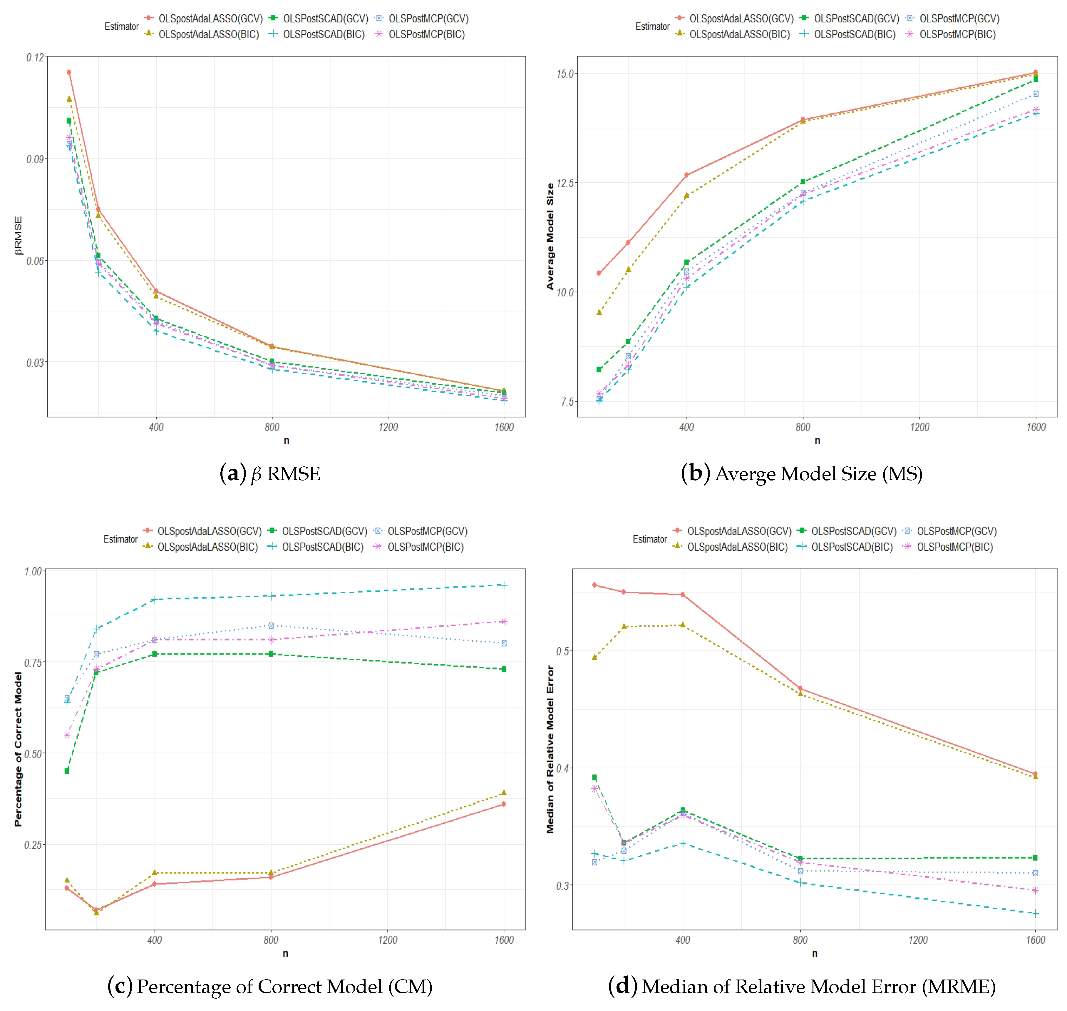
To evaluate the performance of the shrinkage estimators, various measures for variable selection and estimation accuracy have been introduced in the literature. Wang et al. (2009) used the model size (MS), the percentage of the correctly identified true model (CM), and the median of relative model error (MRME) to evaluate the finite sample performances of the adaptive LASSO and SCAD estimators with tuning parameters selected either by the GCV or BIC approach.

The model size, MS, for the true model is defined as the number of nonzero parameters or $|S_0|=p_0$, where $p_0$ is the dimension for the nonzero parameters. For any model selection procedure, ideally, the estimated model size $|\widehat{S}|={\widehat{p}}_0$ should tend to $p_0$ asymptotically, and $\widehat{S}=\{k:{\widehat{\beta }}_k\ne 0\}$. This measure evaluates the precision with which the said selection procedure estimates the number of nonzero parameters from the data. In the context of Monte Carlo simulations, the average is taken over all of the estimated MSs, which are generated per each round of simulation.

The correct model CM is revealed as the true model if the said model selection procedure accurately yields the right nonzero parameters. The CM measure is defined as

$$CM=\left\{\widehat{{\beta }_k}\ne 0:k\in S_0,{\widehat{\beta }}_k=0:k\in {S_0}^c\right\}.$$

(15)

An estimation of the model is only considered correct if the above criterion is satisfied, where all of the non-zero and zero parameters are correctly identified. The higher the correction rate over a number of simulation runs, the better the performance for an estimator.

The model prediction error (ME) for a model selection procedure is defined as

$$ME={(\widehat{\beta }-\beta )}^{T}E\left[X^{T}X\right](\widehat{\beta }-\beta ),$$

(16)

where $\widehat{\beta }$ represents any estimator such as a penalized least squares estimator. The relative model error (RME) is the ratio of the model prediction error to that of the naive OLS estimator of the model given by Equation (1). For example, the RME for the SCAD estimator is given by

$$RME=\frac{{({\widehat{\beta }}^{SCAD}-\beta )}^{T}E\left[X^{T}X\right](({\widehat{\beta }}^{SCAD}-\beta )}{{({\widehat{\beta }}^{OLS}-\beta )}^{T}E\left[X^{T}X\right](({\widehat{\beta }}^{OLS}-\beta )}.$$

(17)

For a given number of Monte Carlo replications, the median of the RME (MRME) is used to evaluate the finite sample performance of the said model selection estimator.

2.2. Model Averaging

On the other hand, an alternative to model selection in handling modeling uncertainties is model averaging. In general, the model averaging estimator is defined as

$${\widehat{\beta }}_{MA}=\sum _{s=1}^{\mathcal{S}}{w}_s{\widehat{\beta }}_s,$$

(18)

where $w_s$ represents the weight assigned to the $s^{th}$ model of an $\mathcal{S}$ number of candidate models, and $w=\left[w_1,w_2\cdots ,w_{\mathcal{S}}\right]$ is a weight vector in the unit simplex in ${\mathbb{R}}^{\mathcal{S}}$ with $\mathcal{S}\in {\mathbb{Z}}^{+}$, such that

$${\mathcal{H}}_{\mathcal{S}}=\left\{w\in {[0,1]}^{\mathcal{S}}:\sum _{s=1}^{\mathcal{S}}{w}_s=1\right\}.$$

(19)

Over time, various estimators have been proposed for estimating the weight vector, w, for averaging the candidate models. Buckland et al. (1997) proposed the smoothed information criterion model averaging estimator, where the weight for the $s^{th}$ model, $w_s$, can be estimated as

$${\widehat{w}}_s^{IC}=\frac{exp(-I_s/2)}{{\sum }_{s=1}^{\mathcal{S}}exp(-I_s/2)},$$

(20)

where $I_s$, the information criterion evaluated at the $s^{th}$ model, is defined as

$$I_s=-2log\left({\widehat{L}}_s\right)+P_s,$$

(21)

with ${\widehat{L}}_s$ being the maximized likelihood value and $P_s$ being the penalty term that takes the form of $2p_s$ for the smoothed Akaike information criterion (S-AIC) and $ln\left(n\right)p_s$ for the smoothed BIC (S-BIC).

Hansen (2007) proposed a Mallows model averaging (MMA) estimator whose weight choice is estimated as

$${\widehat{w}}^{MMA}=\underset{w\in {\mathcal{H}}_{\mathcal{S}}}{argmin}{\left(y-\widehat{\mu }\left(w\right)\right)}^T\left(y-\widehat{\mu }\left(w\right)\right)+2{\sigma }^{2}k\left(w\right),$$

(22)

where the model averaging estimator $\widehat{\mu }\left(w\right)$ is defined as

$$\widehat{\mu }\left(w\right)=\sum _{s=1}^{\mathcal{S}}{w}_s{P}_{s}y=P\left(w\right)y,$$

(23)

and the projection matrix for model s is defined as

$$P_s=X_s{\left(X_s^T{X}_s\right)}^{-1}{X}_s^T.$$

(24)

Moreover, the effective number of parameters, $k\left(w\right)$, is defined as

$$k\left(w\right)=\sum _{s=1}^{\mathcal{S}}{w}_s{k}_s,$$

(25)

where $k_s$ equals the number of parameters in model s. The ${\sigma }^2$ term can be estimated using the variance of a larger model in the set of the candidate models according to Hansen (2007).

Under certain assumptions, Hansen (2007) showed that the MMA minimizes the mean squared prediction error (MSPE), and Gao et al. (2016) showed that the MMA can produce smaller mean squared errors (MSEs) than the OLS estimator. Wan et al. (2010) further relaxed the assumptions of discrete weights and nested regression models that are required by the asymptotic optimality conditions for the MMA to continuous weights without imposing ordering on the predictors.

Hansen and Racine (2012) proposed the heteroskedasticity-consistent jackknife model averaging (JMA) estimator. The weight choice for the JMA estimator is defined as

$${\widehat{w}}^{JMA}=\underset{w\in {\mathcal{H}}_{\mathcal{S}}}{argmin}\frac{1}{n}{\tilde{\epsilon }\left(w\right)}^T\tilde{\epsilon }\left(w\right),$$

(26)

where $\tilde{\epsilon }\left(w\right)={\sum }_{s=1}^{\mathcal{S}}{w}_s{\tilde{\epsilon }}_s$ with ${\tilde{\epsilon }}_s$ being the leave-one-out residual vector from the $s^{th}$ model.

Schomaker (2012) further explored the role of the tuning parameters in the shrinkage averaging estimator (SAE) post model selection. The SAE estimates $\beta$ by averaging over a set of candidate shrinkage estimators, ${\widehat{\beta }}_{\lambda }$, which are calculated with a sequence of tuning parameters. For example, an SAE that averages over an $\mathcal{S}$ number of candidate ${\widehat{\beta }}_{{\lambda }_s}^{LASSO}$ from an $\mathcal{S}$-fold cross-validation procedure can be defined as

$${\widehat{\beta }}_{SAE}=\sum _{s=1}^{\mathcal{S}}{w}_{{\lambda }_s}{\widehat{\beta }}_{{\lambda }_s}^{LASSO},$$

(27)

where ${\lambda }_s\in \{{\lambda }_1,\cdots ,{\lambda }_{\mathcal{S}}\}$ as one of the $\mathcal{S}$ competing tuning parameters. The weights for the SAE are calculated as follows:

$${\widehat{w}}^{SAE}=\underset{w\in {\mathcal{H}}_{\mathcal{S}}}{argmin}\frac{1}{n}{\tilde{\epsilon }\left(w\right)}^T\tilde{\epsilon }\left(w\right),$$

(28)

where $\tilde{\epsilon }\left(w\right)={\sum }_{s=1}^{\mathcal{S}}{w}_{{\lambda }_s}{\tilde{\epsilon }}_s\left({\lambda }_s\right)$ with ${\tilde{\epsilon }}_s\left({\lambda }_s\right)$ being the residual vector for the $s^{th}$ cross-validation.

In this paper, we aim to explore the possibility of combining the model selection and model averaging methods in dealing with modeling uncertainty. We expect that the specifications of the candidate models guided by the appropriate choice of tuning parameter could significantly reduce modeling uncertainty given sparse models.

3. The Shrinkage MMA Estimator

Inspired by the shrinkage averaging estimator (SAE) and the Mallows model averaging (MMA) estimator, we further propose a shrinkage Mallows model averaging (SMMA) estimator to hedge against the possible specification errors from model selection. The SMMA estimator is a two-stage estimator. In the first stage, by applying different penalty estimators introduced in Section 2 with optimal tuning parameters selected via the GCV or BIC method, we obtain a sequence of candidate models. In the second stage, we apply the MMA to estimate $\beta$. The SMMA estimator compliments the class of penalty estimators by allowing for more than one model selection outcome rather than committing to a single model. In addition, this estimator also extends the current MMA framework by introducing a reasonable way to select the set of candidate models to be averaged. The SMMA is especially helpful for averaging high-dimensional candidate models when the generation of such a set of candidate models would be computationally costly if not done via shrinkage approaches. It would be difficult for the traditional MMA to exhaust all possible subsets of candidate models for a high-dimensional dataset. This estimator also builds on the SAE by incorporating the tuning parameter optimization problem, which is crucial to the variable selection process for each candidate model. This estimator is essentially a variation of the MMA estimator, so the asymptotic properties should be similar to those of the MMA.

Lehrer and Xie (2017) briefly mentioned the possibility of having a set of candidate models first shrunk by the LASSO before applying MMA. There is a clear distinction between Lehrer and Xie (2017) and our idea, since the candidate models for averaging are subjectively chosen in Lehrer and Xie (2017), which is the same as the traditional literature on the MMA estimator. However, the SMMA starts with a general, large model and applies different penalty methods to select the candidate models for averaging.

Below we explain the SMMA estimator in detail. Let ${\Lambda }^{Opt}$ be the set of optimal tuning parameters selected either by the BIC or GCV for the model selection procedures introduced in Section 2, and a typical element in ${\Lambda }^{Opt}$ is denoted as ${\widehat{\lambda }}_s^{Opt}$. Therefore ${\Lambda }^{Opt}$ is defined as

$${\Lambda }^{Opt}=\left\{{\widehat{\lambda }}_1^{Opt},\cdots ,{\widehat{\lambda }}_s^{Opt},\cdots ,{\widehat{\lambda }}_{\mathcal{S}}^{Opt}\right\},$$

(29)

where $|{\Lambda }^{Opt}|=\mathcal{S}$.

The SMMA estimator is solved as follows:

$${\widehat{\beta }}_{SMMA}(w;{\Lambda }^{Opt})=\sum _{s=1}^{\mathcal{S}}{\widehat{w}}_s\widehat{\beta }\left({\widehat{\lambda }}_s^{Opt}\right),$$

(30)

where the weight vector is estimated by the MMA criterion,

$$\widehat{w}=\underset{w\in {\mathcal{H}}_{\mathcal{S}}}{argmin}{\left(y-\widehat{\mu }(w;{\Lambda }^{Opt})\right)}^T\left(y-\widehat{\mu }(w;{\Lambda }^{Opt})\right)+2{\sigma }^{2}k(w;{\Lambda }^{Opt}),$$

(31)

and $w=\left[w_1,w_2\cdots ,w_{\mathcal{S}}\right]$ is a weight vector in the unit simplex in ${\mathbb{R}}^{\mathcal{S}}$ with $\mathcal{S}\in {\mathbb{Z}}^{+}$ such that

$${\mathcal{H}}_{\mathcal{S}}=\left\{w\in {[0,1]}^{\mathcal{S}}:\sum _{s=1}^{\mathcal{S}}{w}_s=1\right\}.$$

(32)

The model averaging estimator $\widehat{\mu }\left(w\right)$ is defined as

$$\widehat{\mu }(w;{\Lambda }^{Opt})=\sum _{s=1}^{\mathcal{S}}{w}_{s}P\left({\widehat{\lambda }}_s^{Opt}\right)y=P(w;{\Lambda }^{Opt})y,$$

(33)

where the projection matrix for model s is defined as

$$P\left({\widehat{\lambda }}_s^{Opt}\right)=X^{{\widehat{\lambda }}_s^{Opt}}{\left({X^{{\widehat{\lambda }}_s^{Opt}}}^T{X}^{{\widehat{\lambda }}_s^{Opt}}\right)}^{-1}{X^{{\widehat{\lambda }}_s^{Opt}}}^T,$$

(34)

and the estimator for model s is given by

$$\widehat{\beta }\left({\widehat{\lambda }}_s^{Opt}\right)={\left({X^{{\widehat{\lambda }}_s^{Opt}}}^T{X}^{{\widehat{\lambda }}_s^{Opt}}\right)}^{-1}{X^{{\widehat{\lambda }}_s^{Opt}}}^{T}y.$$

(35)

Let L index the largest model in dimension from the set of the candidate models, i.e.,

$$L=\underset{s\in \mathcal{S}}{argmax}\left|\widehat{\beta }\left({\widehat{\lambda }}_s^{Opt}\right)\right|,$$

(36)

where $|\widehat{\beta }\left({\widehat{\lambda }}_s^{Opt}\right)|$ equals the number of nonzero values in $\widehat{\beta }\left({\widehat{\lambda }}_s^{Opt}\right)$.

Following Hansen (2007), the ${\sigma }^2$ term will be estimated by ${\widehat{\sigma }}_L^2$, which is given below:

$${\widehat{\sigma }}_L^2=\frac{{(y-X_L{\widehat{\beta }}_L)}^T(y-X_L{\widehat{\beta }}_L)}{n-k_L}.$$

(37)

The effective number of parameters $k(w;{\Lambda }^{Opt})$ is defined as

$$k(w;{\Lambda }^{Opt})=\sum _{s=1}^{\mathcal{S}}{w}_{s}k\left({\widehat{\lambda }}_s^{Opt}\right),$$

(38)

where $k\left({\widehat{\lambda }}_s^{Opt}\right)$ = $|\widehat{\beta }\left({\widehat{\lambda }}_s^{Opt}\right)|$.

4. Monte Carlo Simulations

This section assesses the performance of the existing model selection and averaging estimators, including the SMMA estimator proposed in this paper, via a small Monte Carlo simulation experiment. Our data generating process (DGP) is

$$y_i=X_i^T\beta +{\epsilon }_i,\forall i=1,2,\cdots ,n,$$

(39)

where $\beta$ is a $p\times 1$ parameter vector with only $p_0$ number of nonzero parameters.

We further assume that $p_0<p$ and that the error term ${\epsilon }_i\sim i.i.d\mathcal{N}(0,1)$. In addition, $X_i$ is randomly drawn from a p-dimensional multivariate normal distribution with zero mean and a co-variance matrix as follows

$$Cov(X_l,X_j)=\left\{\begin{array}{cc}1,\hfill & \mathrm{if}l=j\hfill \\ 0.5,\hfill & otherwise\hfill \end{array}\right..$$

(40)

To investigate the effect of the number of parameters to sample size ratio ($p/n$) and the degree of model sparsity ($p_0/p$) on the performance of different estimation methods, we consider two data examples in this section. The data example 1 from Section 4.1 considers the case where $p/n$ is constant while $p_0/p$ is decreasing. The data example 2 in Section 4.2 simulates the scenario where $p_0/p$ is constant but $p/n$ decreases as n increases.

4.1. Example 1. Constant $p/n$ Ratio

Similar to the example given in Fan and Peng (2004), we set $\beta ={\left(\frac{11}{4},-\frac{23}{6},\frac{37}{12},-\frac{13}{9},\frac{1}{3},0,\cdots ,0\right)}^T\in {\mathbb{R}}^p$ with $p=n\times \alpha$ for some constant $\alpha$. The nonzero parameters, ${\beta }_0$ , are defined as

$${\beta }_0={\left(\frac{11}{4},-\frac{23}{6},\frac{37}{12},-\frac{13}{9},\frac{1}{3}\right)}^T.$$

(41)

We fix $n=1000$ and allow $\alpha$ to vary in the interval of $\left[0.02,0.98\right]$. Therefore, we consider a case with an increasing number of redundant regressors while the true model remains fixed with 5 nonzero regressors as $\alpha$ increases from .02 to 0.98, where $\alpha =p/n\in \{0.02,0.05,0.1,0.5,0.98\}$ and $p\in \{20,50,100,500,980\}$. If we measure the degree of sparsity by $\delta =1-p_0/p$, we see that the model becomes sparser for larger $\alpha$ and $p_0/p\in \{0.25,0.1,0.05,0.01,0.005\}$. Note that this design allows us to further consider cases where the number of parameters drastically approaches the sample size.

4.2. Example 2. Decreasing $p/n$ Ratio

The second example is similar to Wang et al. (2009), where the dimension of the true model also diverges with the dimension of the full model as n increases. More specifically, $p=\left[7n^{\frac{1}{4}}\right]$ where $\left[a\right]$ stands for the largest integer no larger than a and the size of the true model $|S_0|=p_0=[p/3]$ with ${\beta }_0\sim U(0.5,1.5)$. For sample size $n\in \{100,200,400,800,1600\}$, the respective sizes of the full model are $p\in \{22,26,31,37,44\}$, and the respective sizes of the true model are $S_0\in \{7,8,10,12,14\}$. The number of parameters to sample size ratio is $p/n\in \{0.22,0.13,0.07,0.046,0.027\}$, and the degree of model sparsity is $\delta =2/3$. Different from the example given in Section 4.1, this data example maintains a constant degree of model sparsity.

4.3. Monte Carlo Results

For the simulation studies, we investigated the finite sample performances of the estimators introduced in Section 2 and Section 3. In addition, we also considered the variants of the aforementioned penalized estimators with the tuning parameters selected by the BIC rather than the conventional GCV. To differentiate, we named the OLS post-SCAD with the the tuning parameters selected by the BIC as the OLS post-SCAD(BIC) estimator. We used the finite sample performance of the OLS estimator as the benchmark for those of the model selection and model averaging estimators. For each data example, a total of 500 simulation replications were conducted.

4.3.1. Model Selection Estimators

The penalized least squares estimators considered in the simulation studies are listed in

Table 1. Penalized Estimators.

Estimator
Ridge(GCV)	Ridge(BIC)
OLS post-ridge(GCV)	OLS post-ridge(BIC)
LASSO(GCV)	LASSO(BIC)
OLS post-LASSO(GCV)	OLS post-LASSO(BIC)
Elastic net(GCV)	Elastic net(BIC)
OLS post-elastic net(GCV)	OLS post-elastic net(BIC)
Adaptive LASSO(GCV)	Adaptive LASSO(BIC)
OLS post-adaptive-LASSO(GCV)	OLS post- adaptive LASSO(BIC)
SCAD(GCV)	SCAD(BIC)
OLS post-SCAD(GCV)	OLS post-SCAD(BIC)
MCP(GCV)	MCP(BIC)
OLS post-MCP(GCV)	OLS post-MCP(BIC)

below.

Figure 1 and Figure 2 below present the finite sample performances of the above penalized least squares estimators with the tuning parameters selected by either GCV or BIC. To level the playing field, each estimator was supplied with the same set of candidate tuning parameters $\Lambda =\{{\lambda }^1,\cdots ,{\lambda }^q\}$ as all the other competing estimators, and $|\Lambda |=q$ with $q\in {\mathbb{Z}}^{+}$. Since the conventional LASSO, SCAD, and MCP estimators have already been studied extensively with well-documented finite sample performances, we turn our focus to the finite sample performances of the class of OLS post-selection estimators. For the elastic net estimator, the weights for the $l_1$ penalty and $l_2$ penalty were set to 0.5. For a cleaner representation of comparison and to save space, we choose to report only the first six best-performing OLS post-selection estimators among those listed in Table 1.

Table 2. Performance ranking for the OLS post-selection estimators.

Ranking	Example 1	Example 2
1	OLS post-SCAD(BIC)	OLS post-SCAD(BIC)
2	OLS post-MCP(BIC)	OLS post-MCP(BIC)
3	OLS post-MCP(GCV)	OLS post-MCP(GCV)
4	OLS post-SCAD(GCV)	OLS post-SCAD(GCV)
5	OLS post-LASSO(BIC)	OLS post-adaptive-LASSO(BIC)
6	OLS post-adaptive-LASSO(BIC)	OLS post-adaptive-LASSO(GCV)

below ranks the first six best-performing OLS post-selection estimators based on the results from data example 1 and data example 2.

For both data examples, it is evident from Figures and Figure 2 above that in finite samples, the OLS post-SCAD(BIC) estimator outperforms the competing estimators consistently by yielding lower root mean squared error (RMSE) for $\beta$ and higher selection accuracy. The performance of the OLS post-SCAD(BIC) is also insensitive to the changes in the $p/n$ ratio and the $p_0/p$ ratio. Therefore, as long as $p<n$, our findings show that the OLS post-SCAD(BIC) outperforms the competing OLS post-selection estimators regardless of the effective sample size and degree of model sparsity, which are controlled by $p/n$ and $p_0/p$, respectively. The finite sample performances of the OLS post-LASSO and the OLS post-adaptive-LASSO seem to be affected by changes in the degree of model sparsity and the effective sample size. The simulation results support the conclusion in the literature that the choice of the tuning parameter does play a vital role in the variable selection outcomes. The findings from the two data examples above offer some guidance to empirical researchers who are weighing different approaches for model selection.

4.3.2. Model Averaging Estimators

For the model averaging estimators, we mainly focused on the finite sample performances of the S-BIC, Hansen’s MMA, SAE(LASSO) with LASSO as the shrinkage method, and the SMMA estimator proposed in Section 3. The SMMA estimator averages the candidate models produced by the penalized least squares estimators listed in Table 1. The specifications of the candidate models are determined by the set of optimal tuning parameters ${\Lambda }^{Opt}$, which consists of the optimal tuning parameters selected by either the GCV or the BIC approach. For Hansen’s MMA, we only considered the pure nested subset models due to the fact that all of the possible combinations of subset models are not computationally feasible given the high-dimensional nature of our data examples. Since in Table 1 there are 24 estimators, which yield 24 candidate models, we also generated 24 candidate models for the MMA, S-BIC, and SAE(LASSO). These candidate models were generated using the program developed by Professor Hansen, and the program is available from Professor Hansen’s website. Similar to Hansen (2007), we evaluated the finite sample performances of the model averaging estimators by comparing the $\beta$ RMSE and the adjusted $R^2$ for the final averaged model. Due to the high-dimensional sparse nature of the DGP, using the adjusted $R^2$ helps us avoid the misleadingly high $R^2$ from including many more predictors that might have been irrelevant in the first place. The adjusted $R^2$ can also gauge whether the SMMA could better perform the task of identifying the most relevant regressors, which is one of the fundamental goals for statistical learning.

Figure 3 above gives the finite sample performances of the model averaging estimators from both data examples. For data example 1, where the degree of model sparsity increases while the effective sample size decreases with the increase in the $p/n$, the SMMA outperforms the MMA in terms of yielding a relatively lower $\beta$ RMSE and slightly higher adjusted $R^2$ if $p/n<0.5$. As $p/n$ increases from 0.5 to 0.98, which causes $p_0/p$ to further decrease, resulting in a much sparser model, the SMMA significantly outperforms the competing model averaging estimators in $\beta$ RMSE and adjusted $R^2$. The sparser the model and the smaller the effective sample size, the better the SMMA performs. This supports the application of the SMMA estimator when averaging high-dimensional sparse models against modeling uncertainty. Intuitively, a sparser model entails greater modeling uncertainty, which could result from the lack of a unifying theory in guiding the exact specification of the underlying model. Therefore, the SMMA can be a viable option for model averaging, especially for high-dimensional sparse models when it is computationally infeasible to exhaust all possible combinations of subset models.

For data example 2, where the degree of model sparsity is constant and the $p/n$ decreases as the sample size n increases, the SMMA still slightly outperforms other model averaging estimators in $\beta$ RMSE and adjusted $R^2$. However, the finite sample performances of the SMMA and MMA estimators tend to be very close as n increases, which indicates rather similar asymptotic properties for both estimators. As a possible direction for future research, one could consider the derivation of the asymptotic properties for the SMMA estimator. But this paper focuses on the numerical comparisons of the SMMA, whose asymptotic properties will be for our future research.

5. Conclusions

In this paper, we reviewed some of the conventional model selection and model averaging estimators, and we further proposed a shrinkage Mallows model averaging (SMMA) estimator. Using a Monte Carlo study, we compared the finite sample performances of the reviewed model selection and model averaging estimators. We also investigated the effect of the tuning parameter choice on variable selection outcomes. We aimed to supplement the existing model selection literature by studying the finite sample performances of the class of OLS post-selection estimators via different tuning parameter selection approaches. Our Monte Carlo design further considered the effect of changes in the effective sample size and the degree of model sparsity on the finite sample performances of model selection and model averaging estimators.

The results from our data examples suggest that tuning parameter choice plays a vital role in variable selection and optimal estimation. Given the same tuning parameter selection approach, for the penalized estimators that are already oracle efficient, the corresponding OLS post-selection estimators give a rather similar performance. However, for the same penalized estimators, the performances via different tuning parameter selection approaches are markedly different. The OLS post-SCAD(BIC) estimator gives the best finite sample performance, based on the data examples in our Monte Carlo design. The SMMA performs better given sparser models. The sparser the model and the smaller the effective sample size, the better the SMMA performs. This supports the use of the SMMA estimator when averaging high-dimensional sparse models against modeling uncertainty. This paper is limited by the absence of the derivation of the asymptotic properties for the SMMA estimator. We will leave the derivations of the asymptotic properties for the SMMA estimator to our future studies.

References

1. Belloni, Alexandre, and Victor Chernozhukov. 2013. Least squares after model selection in high-dimensional sparse models. Bernoulli 19: 521–47. [Google Scholar] [CrossRef]
2. Breheny, Patrick, and Jian Huang. 2011. Coordinate descent algorithms for nonconvex penalized regression, with applications to biological feature selection. The Annals of Applied Statistics 5: 232–53. [Google Scholar] [CrossRef] [PubMed]
3. Buckland, Steven T., Kenneth P. Burnham, and Nicole H. Augustin. 1997. Model Selection: An Integral Part of Inference. Biometrics 53. [Google Scholar] [CrossRef]
4. Fan, Jianqing, and Heng Peng. 2004. Nonconcave penalized likelihood with a diverging number of parameters. The Annals of Statistics 32: 928–61. [Google Scholar] [CrossRef]
5. Fan, Jianqing, and Runze Li. 2001. Variable Selection via Nonconcave Penalized Likelihood and Its Oracle Properties. Journal of the American Statistical Association 96: 1348–60. [Google Scholar] [CrossRef]
6. Fan, Jianqing, and Runze Li. 2006. Statistical Challenges with High Dimensionality: Feature Selection in Knowledge Discovery. arXiv arXiv:arXiv:math/0602133. [Google Scholar]
7. Fan, Yingying, and Cheng Yong Tang. 2013. Tuning Parameter Selection in High Dimensional Penalized Likelihood. Journal of the Royal Statistical Society. Series B (Statistical Methodology) 75: 531–52. [Google Scholar] [CrossRef]
8. Gao, Yan, Xinyu Zhang, Shouyang Wang, and Guohua Zou. 2016. Model averaging based on leave-subject-out cross-validation. Journal of Econometrics 192: 139–51. [Google Scholar] [CrossRef]
9. Hansen, Bruce. 2007. Least Squares Model Averaging. Econometrica 75: 1175–89. [Google Scholar] [CrossRef]
10. Hansen, Bruce. 2014. Model averaging, asymptotic risk, and regressor groups. Quantitative Economics 5: 495–530. [Google Scholar] [CrossRef] [Green Version]
11. Hansen, Bruce, and Jeffrey Racine. 2012. Jackknife model averaging. Journal of Econometrics 167: 38–46. [Google Scholar] [CrossRef]
12. Hoerl, Arthur E., and Robert W. Kennard. 1970. Ridge Regression: Biased Estimation for Nonorthogonal Problems. Technometrics 12: 55–67. [Google Scholar] [CrossRef]
13. Knight, Keith, and Wenjiang Fu. 2000. Asymptotics for lasso-type estimators. The Annals of Statistics 5: 1356–78. [Google Scholar] [CrossRef]
14. Lehrer, Steven, and Tian Xie. 2017. Box Office Buzz: Does Social Media Data Steal the Show from Model Uncertainty When Forecasting for Hollywood? Review of Economics and Statistics 99: 749–55. [Google Scholar] [CrossRef]
15. Pötscher, Benedikt M., and Hannes Leeb. 2009. On the Distribution of Penalized Maximum Likelihood Estimators: The LASSO, SCAD, and Thresholding. Journal of Multivariate Analysis 100: 2065–82. [Google Scholar] [CrossRef]
16. Pötscher, Benedikt M., and Ulrike Schneider. 2009. On the Distribution of the Adaptive LASSO Estimator. Journal of Statistical Planning and Inference 139: 2775–90. [Google Scholar] [CrossRef]
17. Schomaker, Michael. 2012. Shrinkage averaging estimation. Statistical Papers 53: 1015–34. [Google Scholar] [CrossRef]
18. Shi, Peide, and Chih-Ling Tsai. 2002. Regression model selection—A residual likelihood approach. Journal of the Royal Statistical Society Series B 64: 237–52. [Google Scholar] [CrossRef]
19. Tibshirani, Robert. 1996. Regression Shrinkage and Selection via the Lasso. Journal of the Royal Statistical Society. Series B (Methodological) 58: 267–88. [Google Scholar] [CrossRef]
20. Tibshirani, Rob, Trevor Hastie, and Jerome Friedman. 2010. Regularization Paths for Generalized Linear Models via Coordinate Descent. Journal of Statistical Software 33: 1–22. [Google Scholar] [CrossRef]
21. Wang, Hansheng, Bo Li, and Chenlei Leng. 2009. Shrinkage Tuning Parameter Selection with a Diverging Number of Parameters. Journal of the Royal Statistical Society. Series B (Statistical Methodology) 71: 671–83. [Google Scholar] [CrossRef]
22. Wan, Alan T. K., Xinyu Zhang, and Guohua Zou. 2010. Least squares model averaging by Mallows criterion. Journal of Econometrics 156: 277–83. [Google Scholar] [CrossRef]
23. Zhang, Cun-Hui. 2010. Nearly unbiased variable selection under minimax concave penalty. The Annals of Statistics 38: 894–942. [Google Scholar] [CrossRef] [Green Version]
24. Zou, Hui, and Trevor Hastie. 2005. Regularization and Variable Selection via the Elastic Net. Journal of the Royal Statistical Society. Series B (Statistical Methodology) 67: 301–20. [Google Scholar] [CrossRef]
25. Zou, Hui. 2006. The Adaptive Lasso and Its Oracle Properties. Journal of the American Statistical Association 101: 1418–29. [Google Scholar] [CrossRef]
Figure 1. Example 1 model selection and estimation accuracy.
Jrfm 12 00109 g001aJrfm 12 00109 g001b
Figure 2. Example 2 model selection and estimation accuracy.
Jrfm 12 00109 g002
Figure 3. Finite sample performance for model averaging estimators.
Jrfm 12 00109 g003