Modeling and Forecasting Realized Portfolio Diversification Benefits

Abstract

For a financial portfolio, we suggest a realized measure of diversification benefits, which is based on intraday high-frequency returns. Our measure quantifies volatility reduction, which could be achieved by including an additional asset in the portfolio. In order to make our approach feasible for investors, we also provide time series modeling of both the realized diversification measure and realized portfolio weight. The performance of our approach is evaluated in-sample and out-of-sample. We find out that our approach is helpful for the purpose of portfolio variance minimization.

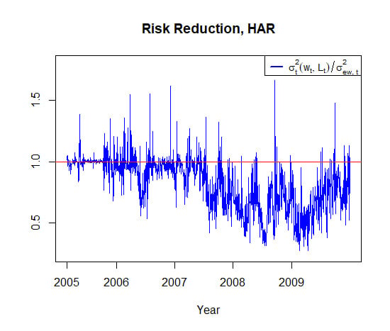
1. Introduction

The mean-variance portfolio selection procedure of Markowitz (1952) remains a theoretical cornerstone of the modern portfolio theory. Empirically, one should not apply the mean-variance portfolio optimization directly, primarily due to the effect of estimation risk in the mean returns; see, e.g., Best and Grauer (1991); Chopra and Ziemba (1993). For this reason, variance minimization approaches leading to the choice of the global minimum variance portfolio (GMVP) (cf. Ledoit and Wolf 2003) or even naive equally-weighted portfolios (cf. DeMiguel et al 2009a, 2009b) often appear to be preferable in practical portfolio selection. Further improvement of the GMVP performance could be gained by imposing constraints on portfolio weights (Jagannathan and Ma 2003), using shrinkage procedures (Golosnoy and Okhrin 2009; Frahm and Memmel 2010), or applying LASSO or other regularization techniques (Callot et al. 2017).

The essential concept of portfolio diversification postulates that non-systematic risks could be substantially reduced by including enough not perfectly-correlated risky assets into the portfolio. Hence, when selecting a portfolio composition, one of the crucial questions is whether the portfolio is already diversified enough or if including additional assets would lead to a further noticeable risk reduction (cf. Evans and Archer 1968). There are various measures of portfolio diversification proposed in the literature; see, e.g., Rudin and Morgan (2006), Bera and Park (2008), Choueifaty and Coignard (2008), Goetzmann and Kumar (2008), or Meucci (2009).

Recently, the work in Frahm and Memmel (2010) suggested to measure diversification as a ratio of the current portfolio variance and the GMVP variance. The work in Frahm and Wiechers (2013) analyzed the properties of this measure and showed that it possesses a convenient economic interpretation. The availability of intraday returns allows computing daily realized variances and covariances of risky asset returns, which are consistent estimators of the daily covariance matrix (Barndorff-Nielsen and Shephard 2004). By analogy, one could also calculate daily realized GMVP weights, which are a function of the realized covariance matrix (cf. Golosnoy et al. 2019). In this paper, we propose a daily realized portfolio diversification measure, which quantifies a portfolio volatility reduction due to inclusion of an additional asset. Our statistic could be seen as a realized extension of the diversification measure of Frahm and Wiechers (2013). We provide its stochastic properties for a given realized covariance matrix estimator.

As investors intend to make portfolio decisions for the next period, it is of interest to predict the next period (day) diversification gains. Hence, we model realized diversification benefits ex-ante and directly in order to obtain the corresponding forecasts. For this purpose, we consider several time series models for our realized diversification measure. Forecasts provided by these models help an investor to decide whether it is reasonable to include or not to include an additional risky asset into the portfolio composition. We found out that the cascade HAR model of Corsi (2009) appears to be mostly suitable in our empirical application both in-sample and out-of-sample, so that it is shown to be reasonable to consider realized diversification statistics.

The rest of the paper is organized as follows: In Section 2, we introduce our realized diversification measure and establish its asymptotic stochastic properties. In Section 3, we propose time series models for diversification in order to make forecasting decisions whether to include additional assets into the portfolio. Then, in Section 4, we provide the empirical study where we estimate the time series models for diversification measures and evaluate the economic relevance of the corresponding diversification forecasts. In Section 5, we conclude the paper, whereas some theoretical results are placed in Appendix A.

2. Realized Measure of Diversification Benefits

2.1. Quantifying Diversification Benefits

Consider a portfolio of risky assets with log-price $p_p(\tau )$ and an additional asset (not included in this portfolio yet) with log-price $p_a(\tau )$ where $\tau \in I{R}_{+}$ represents continuous time. Denote the bivariate vector of their log-prices $p(\tau )={(p_p(\tau ),p_a(\tau ))}^{\prime }$, and assume that $p(\tau )$ is a Brownian stochastic semimartingale with a spot covariance matrix $\mathsf{\Theta }(\tau )$. The integrated covariance matrix at day t is denoted by ${\mathsf{\Sigma }}_t$ with:

$$\begin{array}{c}\hfill {\mathsf{\Sigma }}_t={\int }_{t-1}^t\mathsf{\Theta }(\tau )d\tau =\left(\begin{array}{cc}{\sigma }_{p,t}^2& {\sigma }_{pa,t}\\ {\sigma }_{pa,t}& {\sigma }_{a,t}^2\end{array}\right),\end{array}$$

(1)

where ${\sigma }_{p,t}^2$ and ${\sigma }_{a,t}^2$ are the daily variances of the initial portfolio and the additional asset returns, respectively, and ${\sigma }_{pa,t}$ denotes the corresponding covariance, so that $\mathrm{vech}({\mathsf{\Sigma }}_t)={({\sigma }_{p,t}^2,{\sigma }_{pa,t},{\sigma }_{a,t}^2)}^{\prime }$. Further, we assume that the matrix ${\mathsf{\Sigma }}_t$ is positive definite for all t.

For day t, the log returns on the initial portfolio are $x_{p,t}=p_p(t)-p_p(t-1)$ and on the asset $x_{a,t}=p_a(t)-p_a(t-1)$. Construct a new portfolio with log return $x_t$, which is a linear combination of returns on the initial portfolio $x_{p,t}$ and on the asset $x_{a,t}$:

$$\begin{array}{c}\hfill x_t=v_t{x}_{p,t}+(1-v_t)x_{a,t}.\end{array}$$

(2)

The daily variance of the new portfolio return is denoted by ${\sigma }_t^2$.

This problem can be reformulated as a task of constructing a two-asset (the original portfolio and the additional asset) GMVP, where the corresponding GMVP weight is obtained as a solution of the variance minimization task:

$$\begin{array}{c}\hfill w_t=\underset{v_t}{\arg min}\left[Var(x_t)=Var(v_t{x}_{p,t}+(1-v_t)x_{a,t})\right].\end{array}$$

(3)

The solution of the task (3) is the weight of the original portfolio, which is given by:

$$\begin{array}{c}\hfill w_t=\frac{{\sigma }_{a,t}^2-{\sigma }_{pa,t}}{{\sigma }_{a,t}^2+{\sigma }_{p,t}^2-2{\sigma }_{pa,t}}.\end{array}$$

(4)

The variance of the new GMVP obtained by combining the original portfolio with the additional asset is given as:

$$\begin{array}{c}\hfill {\sigma }_t^2=\frac{{\sigma }_{a,t}^2{\sigma }_{p,t}^2-{\sigma }_{pa,t}^2}{{\sigma }_{a,t}^2+{\sigma }_{p,t}^2-2{\sigma }_{pa,t}}.\end{array}$$

(5)

In line with Frahm and Wiechers (2013), we argue that a statistic that measures the distance between ${\sigma }_t^2$ and ${\sigma }_{p,t}^2$ is of great interest: when ${\sigma }_{p,t}^2$ is substantially larger than ${\sigma }_t^2$, then there are diversification benefits to achieve by including this additional asset into the portfolio. The diversification benefits could be quantified by the variance ratio $D_t$, which is defined as:

$$\begin{array}{c}\hfill D_t=\frac{{\sigma }_{p,t}^2}{{\sigma }_t^2}-1=\frac{{\sigma }_{a,t}^2+{\sigma }_{p,t}^2-2{\sigma }_{pa,t}}{{\sigma }_{a,t}^2-{\sigma }_{a,t}^2{\rho }_{pa,t}^2}-1=\frac{{\sigma }_{a,t}^2{\rho }_{pa,t}^2+{\sigma }_{p,t}^2-2{\sigma }_{pa,t}}{{\sigma }_{a,t}^2(1-{\rho }_{pa,t}^2)}=\frac{{({\sigma }_{p,t}^2-{\sigma }_{pa,t})}^2}{{\sigma }_{a,t}^2{\sigma }_{p,t}^2-{\sigma }_{pa,t}^2},\end{array}$$

(6)

with ${\rho }_{pa,t}={\sigma }_{pa,t}/({\sigma }_{p,t}{\sigma }_{a,t})$. As it holds that ${\sigma }_{a,t}^2{\sigma }_{p,t}^2-{\sigma }_{pa,t}^2>0$ due to the positive definiteness of the matrix ${\mathsf{\Sigma }}_t$, the case ${\sigma }_{p,t}^2={\sigma }_{pa,t}$ is excluded as well. Hence, $D_t\in (0,+\infty )$, and the value of $D_t$ close to zero indicates no reasonable diversification effect from including this asset in the existing portfolio.

However, for our purposes, it is more convenient to consider the log measure:

$$\begin{array}{c}\hfill L_t=\ln D_t=\ln \left(\frac{{\sigma }_{p,t}^2}{{\sigma }_t^2}-1\right)=\ln \frac{{({\sigma }_{p,t}^2-{\sigma }_{pa,t})}^2}{{\sigma }_{a,t}^2{\sigma }_{p,t}^2-{\sigma }_{pa,t}^2}.\end{array}$$

(7)

As the log measure $L_t\in (-\infty ,\infty )$, it appears to be advantageous from the perspective of time series modeling.

2.2. Realized Measures for Diversification

The availability of intraday high-frequency returns provides the possibility to construct precise realized volatility measures. Using them, we introduce the realized diversification measure ${\widehat{D}}_t$ and analyze its asymptotic stochastic properties.

Assume that we observe m intraday log-prices for day t at uniformly-spaced time intervals. Then, the jth intraday return vector is given by:

$$\begin{array}{c}\hfill x_{t,j}=p\left((t-1)+j/m\right)-p\left((t-1)+(j-1)/m\right),j=1,\cdots ,m.\end{array}$$

(8)

These high-frequency intraday returns appear to be useful for the construction of the realized covariance measures, which are precise nonparametric ex-post estimates of ${\mathsf{\Sigma }}_t$. The most simple realized covariance matrix estimator is given as:

$$\begin{array}{c}\hfill {\widehat{\mathsf{\Sigma }}}_t=\sum _{j=1}^m{x}_{t,j}{x}_{t,j}^{\prime }.\end{array}$$

(9)

Accordingly, for the entries of matrix ${\mathsf{\Sigma }}_t$, we get the realized estimators ${\widehat{\sigma }}_{a,t}^2={\sum }_{j=1}^m{x}_{a,t,j}^2$, ${\widehat{\sigma }}_{p,t}^2={\sum }_{j=1}^m{x}_{p,t,j}^2$, and ${\widehat{\sigma }}_{pa,t}={\sum }_{j=1}^m{x}_{p,t,j}{x}_{a,t,j}$. More advanced estimators, such as the realized kernel or composite realized kernel (cf. Lunde et al. 2016), are proposed in order to provide more elaborated realized volatility estimators.

Given the realized covariance matrix ${\widehat{\mathsf{\Sigma }}}_t$, the realized diversification measure ${\widehat{D}}_t$ is defined as:

$$\begin{array}{c}\hfill {\widehat{D}}_t=\frac{{({\widehat{\sigma }}_{p,t}^2-{\widehat{\sigma }}_{pa,t})}^2}{{\widehat{\sigma }}_{a,t}^2{\widehat{\sigma }}_{p,t}^2-{\widehat{\sigma }}_{pa,t}^2}.\end{array}$$

For time series modeling purposes, it appears to be more convenient to consider the measure ${\widehat{L}}_t=\ln {\widehat{D}}_t$, as its distribution is not as skewed as those of ${\widehat{D}}_t$. We formulate the stochastic properties of both ${\widehat{D}}_t$ and ${\widehat{L}}_t$ in the following proposition, which is proven in Appendix A.

Proposition 1.

Consider a realized covariance matrix measure ${\widehat{\mathsf{\Sigma }}}_t$ in (9), which is a consistent estimator of the positive definite covariance matrix ${\mathsf{\Sigma }}_t$ for the number of intraperiod returns $m\to \infty$. Then, the realized diversification measure ${\widehat{D}}_t={({\widehat{\sigma }}_{p,t}-{\widehat{\rho }}_{pa,t}{\widehat{\sigma }}_{a,t})}^2/({\widehat{\sigma }}_{a,t}^2{\widehat{\sigma }}_{p,t}^2-{\widehat{\sigma }}_{pa,t}^2)$ is a consistent estimator of the diversification benefit $D_t$. Moreover, given that $m^{1/2}(vech({\widehat{\mathsf{\Sigma }}}_t)-vech({\mathsf{\Sigma }}_t))\stackrel{L}{⟶}\mathcal{N}(0,{\mathsf{\Pi }}_t)$ for $m\to \infty$ with $\stackrel{L}{⟶}$ indicating convergence in the distribution (law), the estimator ${\widehat{D}}_t$ is asymptotically normally distributed with:

$$\begin{array}{c}\hfill m^{1/2}({\widehat{D}}_t-D_t)\stackrel{L}{⟶}\mathcal{N}(0,{(\nabla D_t)}^{\prime }{\mathsf{\Pi }}_t\nabla D_t).\end{array}$$

The expression for ${\mathsf{\Pi }}_t$ was provided by Barndorff-Nielsen and Shephard (2004); its realized estimator ${\widehat{\mathsf{\Pi }}}_t$ is given in (A1) in Appendix A, whereas the gradient is given by:

$$\begin{array}{c}\hfill \nabla D_t=\frac{{\sigma }_{p,t}^2-{\sigma }_{pa,t}}{{({\sigma }_{a,t}^2{\sigma }_{p,t}^2-{\sigma }_{pa,t}^2)}^2}·{\left({\sigma }_{a,t}^2({\sigma }_{p,t}^2+{\sigma }_{pa,t})-2{\sigma }_{pa,t}^2,2{\sigma }_{p,t}^2({\sigma }_{pa,t}-{\sigma }_{a,t}^2),-{\sigma }_{p,t}^2({\sigma }_{p,t}^2-{\sigma }_{pa,t})\right)}^{\prime }.\end{array}$$

Next, the estimator ${\widehat{L}}_t$ of $L_t$ is also consistent and asymptotically normally distributed for $m\to \infty$ with:

$$\begin{array}{c}\hfill m^{1/2}({\widehat{L}}_t-L_t)\stackrel{L}{⟶}\mathcal{N}(0,{(\nabla L_t)}^{\prime }{\mathsf{\Pi }}_t\nabla L_t),\end{array}$$

(10)

with the gradient given as:

$$\nabla L_t={\left(\frac{2}{{\sigma }_{p,t}^2-{\sigma }_{pa,t}}-\frac{{\sigma }_{a,t}^2}{{\sigma }_{a,t}^2{\sigma }_{p,t}^2-{\sigma }_{pa,t}^2},\frac{2{\sigma }_{pa,t}}{{\sigma }_{a,t}^2{\sigma }_{p,t}^2-{\sigma }_{pa,t}^2}-\frac{2}{{\sigma }_{p,t}^2-{\sigma }_{pa,t}},\frac{-{\sigma }_{p,t}^2}{{\sigma }_{a,t}^2{\sigma }_{p,t}^2-{\sigma }_{pa,t}^2}\right)}^{\prime }.$$

A similar asymptotic distribution for the optimal realized weight ${\widehat{w}}_t$ could be obtained as a special case of the Theorem 1 result in Golosnoy et al. (2019). We provide the asymptotic variance of ${\widehat{w}}_t$ in Appendix A, together with the asymptotic covariances $ACov({\widehat{w}}_t,{\widehat{D}}_t)$ and $ACov({\widehat{w}}_t,{\widehat{L}}_t)$ for $m\to \infty$.

The distributional result in Equation (10) in Proposition 1 would be of particular importance for making tests for the usefulness of the additional asset in the portfolio composition. For example, the null hypotheses $H_0:D_t=D_0$ can be tested by means of the statistic:

$$\begin{array}{ccc}\hfill T_{D,t}& =& \sqrt{m}\frac{{\widehat{D}}_t-D_0}{\sqrt{{(\widehat{\nabla }{D}_t)}^{\prime }{\widehat{\mathsf{\Pi }}}_t\widehat{\nabla }{D}_t}}\stackrel{H_0}{\sim }\mathcal{N}(0,1).\hfill \end{array}$$

(11)

If this statistic $T_{D,t}$ is smaller than the $\alpha$-quantile of the $\mathcal{N}(0,1)$ distribution, no significant diversification benefits can be achieved by including the additional asset into the portfolio. The test for $H_0:L_t=L_0$ could be conducted by analogy with the test statistic:

$$\begin{array}{ccc}\hfill T_{L,t}& =& \sqrt{m}\frac{{\widehat{L}}_t-L_0}{\sqrt{{(\widehat{\nabla }{L}_t)}^{\prime }{\widehat{\mathsf{\Pi }}}_t\widehat{\nabla }{L}_t}}\stackrel{H_0}{\sim }\mathcal{N}(0,1).\hfill \end{array}$$

(12)

To illustrate the results in Proposition 1, we conducted a Monte Carlo simulation study, which was designed as follows. For $T={10}^4$ days, we drew m intraday returns ${\mathbf{x}}_t={(x_{t,p},x_{t,a})}^{\prime }$ from a bivariate normal distribution with ${\mathbf{x}}_t\sim \mathcal{N}\left(\mathbf{0},m^{-1}\mathsf{\Sigma }\right)$ and $vech(\mathsf{\Sigma })={(1,{\sigma }_{pa,t},1)}^{\prime }$. We performed this simulation study for $m=78$ corresponding to 5-min intraday sampling and for $m=390$ corresponding to 1-min intraday sampling. We selected the correlation ${\sigma }_{pa,t}\in [0,0.3,0.5]$. Relying on the results from Proposition 1, we computed (11) and (12) for each $t=1,\dots ,T$ and then calculated the sample moments—mean, variance, skewness, kurtosis—as well as applied the Kolmogorov–Smirnov (KS) and Jarque–Bera (JB) test to check whether (11) and (12) followed a standard normal distribution. The values $D_0$ and $L_0$ were set to the true value for the given matrix $\mathsf{\Sigma }$.

From the results reported in

Table 1. Sample moments and p-values of Kolmogorov–Smirnov and Jarque–Bera tests for normality.

Block A: Monte Carlo Simulation Results for ${\mathit{T}}_{\mathit{D}}$
m	${\mathit{\sigma }}_{\mathit{pa},\mathit{t}}$	Mean	Variance	Skewness	Kurtosis	${\mathit{p}}_{\mathit{KS}}$	${\mathit{p}}_{\mathit{JB}}$
78	0	−0.064	$1.188$	−0.979	$5.374$	$0.051$	0
	0.3	−0.072	$1.133$	−0.855	$4.421$	$0.183$	0
	0.5	−0.098	$1.203$	−0.999	$5.067$	$0.098$	0
390	0	−0.056	1.054	−0.198	$3.113$	$0.576$	$0.029$
	0.3	−0.033	$1.001$	−0.383	$3.290$	$0.458$	0
	0.5	−0.039	$1.004$	−0.419	$3.359$	$0.341$	0
Block B: Monte Carlo Simulation Results for ${\mathit{T}}_{\mathit{L}}$
$\mathit{m}$	${\mathit{\sigma }}_{\mathit{pa},\mathit{t}}$	Mean	Variance	Skewness	Kurtosis	${\mathit{p}}_{\mathit{KS}}$	${\mathit{p}}_{\mathit{JB}}$
78	0	$0.105$	$1.049$	$0.210$	$3.234$	$0.048$	$0.008$
	0.3	$0.122$	$0.998$	$0.403$	$3.288$	$0.070$	0
	0.5	$0.138$	$0.997$	$0.557$	$3.462$	$0.019$	0
390	0	$0.018$	$1.046$	$0.239$	$3.088$	$0.732$	$0.007$
	0.3	$0.051$	$0.971$	$0.141$	$3.066$	$0.357$	$0.175$
	0.5	$0.060$	$0.963$	$0.195$	$3.018$	$0.378$	$0.042$

Note: computed by generating $T={10}^4$ days with $m=78$ or $m=390$ intraday returns.

, we could observe that the sample moments were much better matched by $T_L$ compared to $T_D$. The p-values of the KS and JB tests indicated that at intraday sampling frequency $m=78$, the assumption of normality could be rejected in some cases. However, for $m=390$, both $D_t$- and $L_t$-based test statistics appeared to be quite close to the null hypothesis of the standard normal distribution.

3. Time Series Model for Diversification Measures

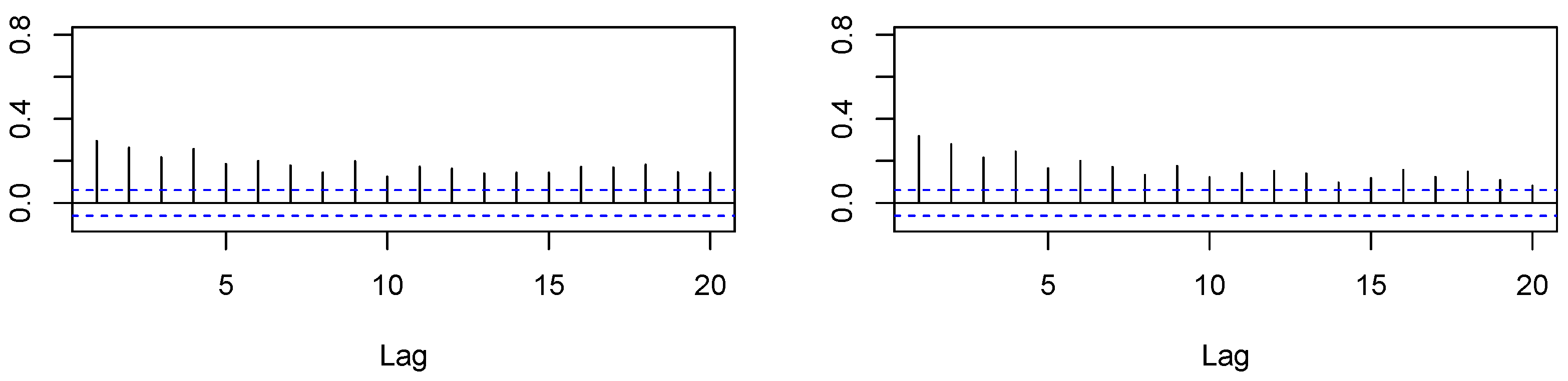
The realized diversification measures ${\widehat{D}}_t$ and ${\widehat{L}}_t$ are observable at the end of period (day) t. However, the investor should decide whether to include or not the additional asset into the portfolio already at $t-1$. Hence, it is necessary to forecast the diversification measures based on the information set ${\mathcal{F}}_{t-1}$ in order to facilitate the investment decisions. Since the measure $D_t$ is a function of ${\sigma }_{p,t}^2$, ${\sigma }_{a,t}^2$ and ${\sigma }_{pa,t}$, we expect that both time series of ${\widehat{D}}_t$ and ${\widehat{L}}_t$ would exhibit similar properties, such as slowly decaying autocorrelation functions, which is also supported by the empirical evidence in Section 4. Next, we concentrate on time series modeling of the observable realized measures ${\widehat{L}}_t$.

To capture the persistency of $D_t$, we utilized the Heterogeneous Autoregressive (HAR) model proposed by Corsi (2009), which is a natural choice for modeling log realized volatility series. The HAR models have several advantages for our purposes. First, they can be estimated by a simple application of the Ordinary Least Squares (OLS) methodology. Second, the model is sparsely parameterized so that only a few parameters need to be estimated. Third, the model is able to accommodate easily various shocks due to its cascade nature, which makes the HAR approach rather robust. The HAR model for ${\widehat{D}}_t$ is defined as:

$$\begin{array}{c}\hfill {\widehat{D}}_t=c+{\beta }_d{\widehat{D}}_{t-1}+{\beta }_w{\widehat{D}}_t^{(w)}+{\beta }_m{\widehat{D}}_t^{(m)}+{\epsilon }_t,{\epsilon }_t\sim i.i.d.(0,{\sigma }_{\epsilon }^2),\end{array}$$

(13)

with ${\widehat{D}}_t^{(w)}=(1/5)·{\sum }_{i=1}^5{\widehat{D}}_{t-i}$ and ${\widehat{D}}_t^{(m)}=(1/22)·{\sum }_{i=1}^{22}{\widehat{D}}_{t-i}$. Hence, the HAR model postulates that the current $D_t$ depends on the previous day $D_{t-1}$, as well as on averages over the last week and over last month. By analogy, we specify the model for ${\widehat{L}}_t$:

$$\begin{array}{ccc}\hfill {\widehat{L}}_t& =& c+{\beta }_d{\widehat{L}}_{t-1}+{\beta }_w{\widehat{L}}_t^{(w)}+{\beta }_m{\widehat{L}}_t^{(m)}+{\epsilon }_t,\hfill \end{array}$$

(14)

with ${\widehat{L}}_t^{(w)}=\ln \left[(1/5)·{\sum }_{i=1}^5{\widehat{D}}_{t-i}\right]$, etc.

For making investment decisions at $t-1$, it is also of importance to forecast the GMVP weight $w_t$ based on the information set ${\mathcal{F}}_{t-1}$. As the time series properties of realized ${\widehat{w}}_t$ are rather similar to those of the realized volatilities, we applied for ${\widehat{w}}_t$ the HAR model as well with:

$$\begin{array}{c}\hfill {\widehat{w}}_t=c+{\beta }_d{\widehat{w}}_{t-1}+{\beta }_w{\widehat{w}}_t^{(w)}+{\beta }_m{\widehat{w}}_t^{(m)}+{\epsilon }_t,\end{array}$$

(15)

with ${\widehat{w}}_t^{(w)}=(1/5)·{\sum }_{i=1}^5{\widehat{w}}_{t-i}$, etc. The corresponding one-step-ahead forecasts are denoted as ${\tilde{D}}_t$, ${\tilde{L}}_t$, and ${\tilde{w}}_t$. The HAR-type models in (13)–(15) are estimated by the OLS methodology in Section 4.

4. Empirical Application

We structure our empirical study in the following way. First, we describe the data and construction of the portfolios in Section 4.1. Second, we estimate the time series models and provide the corresponding diagnostics in Section 4.2, where we compare the HAR approaches with simple AR(1) and AR(5) alternatives. Finally, in Section 4.3, we evaluate the performance of our approach by investigating whether our measures are suitable for reducing the portfolio variance from the investors’ perspective.

4.1. Data and Construction of Portfolios

Our sample consisted of 10 stocks listed in Table 1 ranging from 1 February 2001–31 December 2009 with $T=2242$ observations in total. This sample was investigated by Noureldin et al. (2012) and is available through Heber et al. (2009). We used the period until 28 February 2005 with 1022 observations as the in-sample to estimate our models.

Table 2. Average realized daily variances of assets and portfolios.

Company	In-Sample	Out-of-Sample	% Change from In- to Out-of-Sample	Portfolio
Bank of America	1.68	8.63	414.64	$\left.\phantom{\begin{array}{c}\hfill c\end{array}}\right\}{P}_{\mathrm{high}}$
Alcoa	3.32	6.30	89.76
American Express	3.16	5.47	73.23
J.P. Morgan	3.93	6.00	52.69
Exxon	1.73	2.36	36.15
General Electric	2.69	3.62	34.20	$\left.\phantom{\begin{array}{c}\hfill c\end{array}}\right\}{P}_{\mathrm{low}}$
DuPont	2.25	2.76	22.93
IBM	2.05	1.84	−10.49
Microsoft	2.91	2.07	−28.82
Coca Cola	1.68	1.19	−29.18
$P_{ew}$	1.10	1.92	75.13
$P_{\mathrm{low}}$	1.21	1.27	5.01
$P_{\mathrm{high}}$	1.31	3.28	150.29

Note: in-sample: 1 February 2001–28 February 2005, 1022 obs.; out-of-sample: 1 March 2005–31 December 2009, 1220 obs.

displays the average in-sample and out-of-sample daily realized variances of all assets.

For our purposes, we constructed three portfolios, namely the equally-weighted portfolio with 10 assets denoted as $P_{ew}$, as well as two equally weighted portfolios from five stocks each with the highest and lowest average in-sample daily realized variances, denoted as $P_{\mathrm{high}}$ and $P_{\mathrm{low}}$, respectively. In the out-of-sample period, which was manifested by the subprime mortgage crisis 2007–2009, the average portfolio variance increased compared to the in-sample period by 150.29% for $P_{\mathrm{high}}$, by 75.13% for $P_{ew}$, and only by 5.01% for $P_{\mathrm{low}}$.

We consider now the following setting: the investor holds the portfolio $P_{\mathrm{low}}$ and considers the possibility to reduce the portfolio risk by including the portfolio $P_{\mathrm{high}}$ as an additional asset. For this approach, we computed the realized diversification measures ${\widehat{L}}_t$ and the realized GMVP weights ${\widehat{w}}_t$, which correspond to the proportion of $P_{\mathrm{low}}$ in the new portfolio.

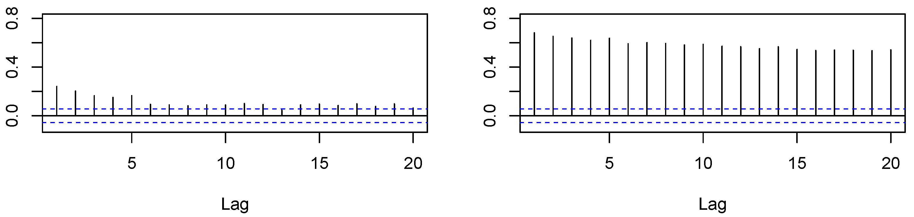
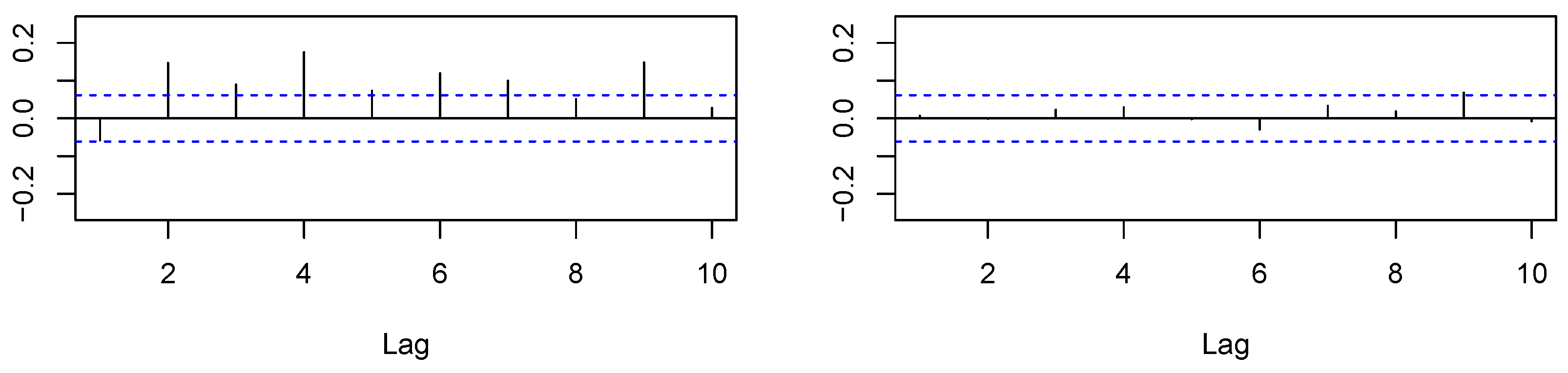
In Figure 1 and Figure 2, we provide the autocorrelation function for ${\widehat{L}}_t$ and ${\widehat{w}}_t$ for both the in-sample and out-of-sample. Both measures appeared to be rather persistent, which is also taken into account by time series modeling in Section 4.2.

4.2. Time Series Modeling

For time series modeling of ${\widehat{L}}_t$ and ${\widehat{w}}_t$, we applied the HAR models as in (14) and (15). Moreover, we considered both the AR(1) and AR(5) models as simple benchmarks for both processes with, e.g., AR(5) for the realized ${\widehat{L}}_t$, parameterized as:

$$\begin{array}{c}\hfill {\widehat{L}}_t=c+{\varphi }_1{\widehat{L}}_{t-1}+{\varphi }_2{\widehat{L}}_{t-2}+{\varphi }_3{\widehat{L}}_{t-3}+{\varphi }_4{\widehat{L}}_{t-4}+{\varphi }_5{\widehat{L}}_{t-5}+{ϵ}_t.\end{array}$$

All three models were estimated by OLS with the results reported in

Table 3. Time series model estimates, ${\widehat{L}}_t$.

Parameter	In-Sample			Full Sample
	HAR	AR(5)	AR(1)	HAR	AR(5)	AR(1)
c	$-\underset{(0.1443)}{0.4029}$ ***	$-(0.1067)0.8895$ ***	$-\underset{(0.0797)}{1.5080}$ ***	$-\underset{(0.1215)}{0.4756}$ ***	$-\underset{(0.0893)}{1.0520}$ ***	$-\underset{(0.0674)}{1.8687}$ ***
${\varphi }_1$ or ${\beta }_d$	$\underset{(0.0347)}{0.1039}$ ***	$\underset{(0.0314)}{0.1877}$ ***	$\underset{(0.0299)}{0.2941}$ ***	$\underset{(0.0234)}{0.1174}$ ***	$\underset{(0.0211)}{0.1958}$ ***	$\underset{(0.0201)}{0.3112}$ ***
${\varphi }_2$		$\underset{(0.0316)}{0.1356}$ ***			$\underset{(0.0214)}{0.1376}$ ***
${\varphi }_3$		$\underset{(0.0318)}{0.0708}$ **			$\underset{(0.0215)}{0.0845}$ ***
${\varphi }_4$		$\underset{(0.0317)}{0.1461}$ ***			$\underset{(0.0214)}{0.1005}$ ***
${\varphi }_5$		${\underset{(0.0314)}{0.0466}}^{}$			$\underset{(0.0211)}{0.0957}$ ***
${\beta }_w$	$\underset{(0.0981)}{0.3743}$ ***			$\underset{(0.0675)}{0.4651}$ ***
${\beta }_m$	$\underset{(0.1234)}{0.5586}$ ***			$\underset{(0.0852)}{0.4962}$ ***
AIC	$3598.5$	$3677.5$	$3762.0$	$8896.7$	$9002.7$	$9189.6$
BIC	$3623.0$	$3711.9$	$3776.7$	$8925.2$	$9042.7$	$9206.8$
adjusted ${\overline{R}}^2$	$0.160$	$0.147$	$0.086$	$0.176$	$0.163$	$0.096$

Standard errors are reported in parentheses; p-values: * <10%, ** <5%, *** <1%.

.

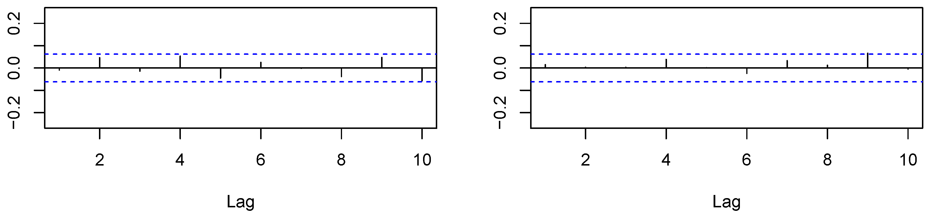
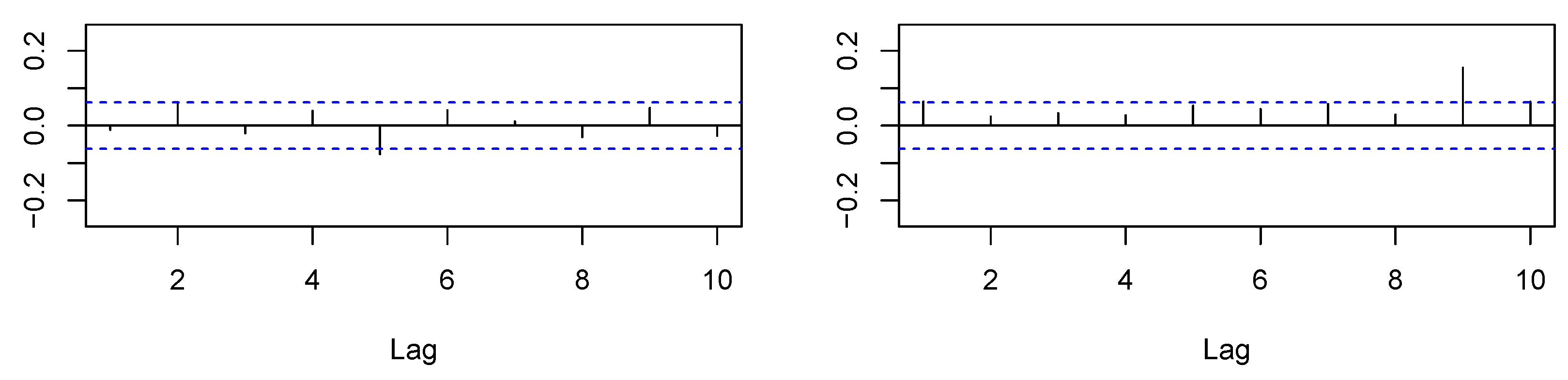
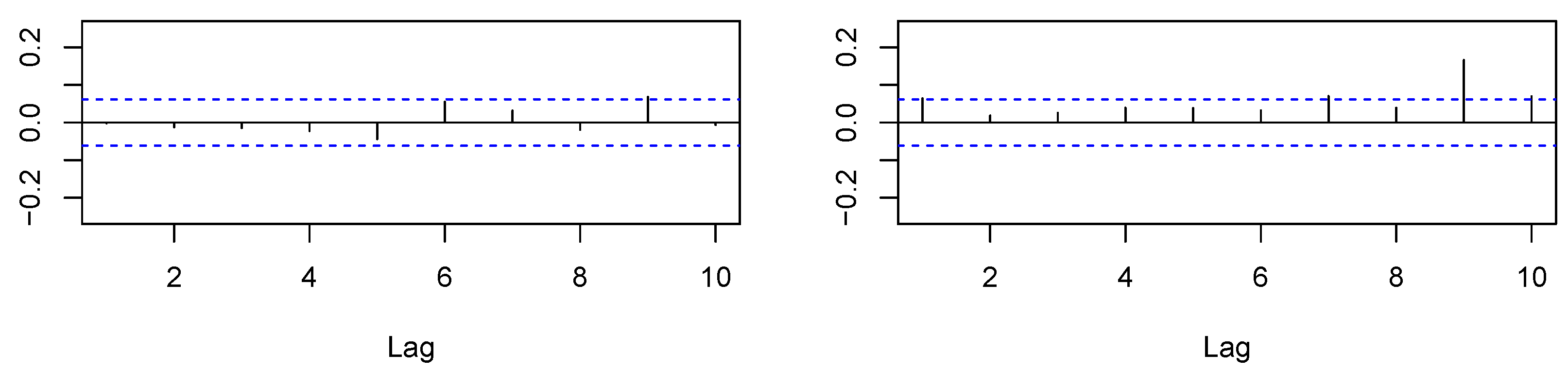
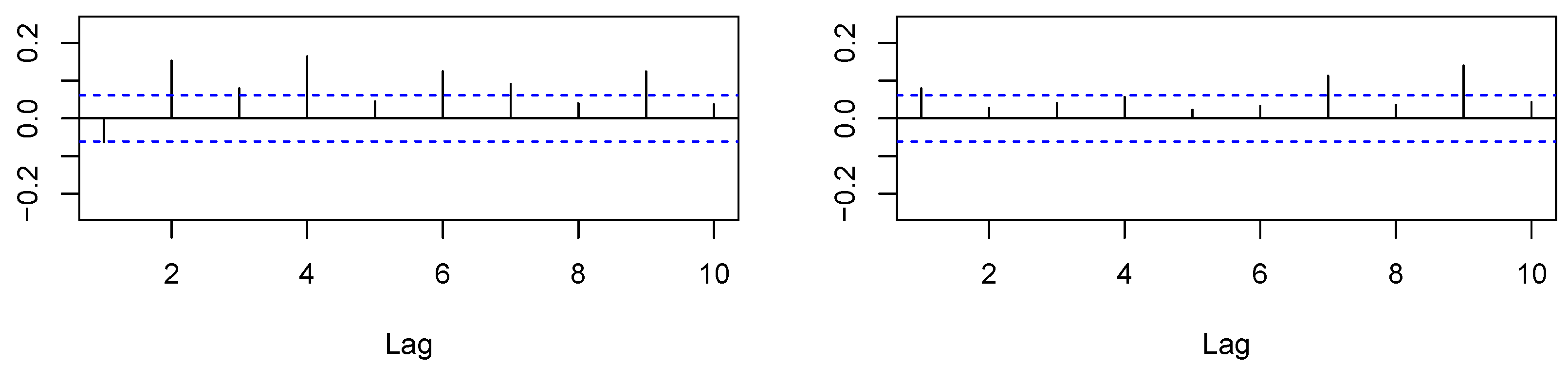
Almost all model coefficients proved to be significantly different from zero. Considering the ${\overline{R}}^2$, the HAR model gave the best fit, followed by the AR(5). Moreover, the AR(5) and HAR both had lower values for AIC and BIC than the AR(1) model. Next, we analyzed the in-sample regression residuals to further check the models’ adequacy. In Figure 3, Figure 4 and Figure 5, we show the Autocorrelation Functions (ACF) of the models’ residuals and their squares.

Based on the ACF plots, we conclude that our HAR and AR(5) modeling removed residual autocorrelation, whereas some autocorrelation remained for the AR(1) approach. Furthermore, there appeared to be no autocorrelation in the squared residuals for all models. Additionally, in

Table 4. ${\widehat{L}}_t$, in-sample residual diagnostic test statistics. LB, Ljung–Box; SW, Shapiro–Wilk.

	HAR	AR(5)	AR(1)
LB(5)	7.299 (0.199)	3.255 (0.661)	70.890 (6.7 $\times {10}^{-14}$)
ARCH-LM	1.686 (0.891)	3.866 (0.569)	1.408 (0.923)
SW	0.843 (<2.2 $\times {10}^{-16}$)	0.844 (<2.2 $\times {10}^{-16}$)	0.850 (<2.2 $\times {10}^{-16}$)

The corresponding p-values are reported in parentheses.

, we provide the results of residual tests, namely the Ljung–Box (LB) test for autocorrelation, the ARCH-LM test for heteroskedasticity, and Shapiro–Wilk (SW) test for the normality assumption.

Supporting the evidence from the ACF plots, the tests failed to reject the null hypotheses of no serial correlation and no ARCH effects for the HAR and AR(5) models. On the other hand, the Ljung–Box test rejected the null “no autocorrelation” for AR(1), indicating that this model does not reflect the underlying dynamics well enough. The normality assumption was clearly rejected for all models.

Next, we estimated the HAR, AR(5), and AR(1) models for the process of realized weights ${\widehat{w}}_t$, with, e.g., the AR(5) model given as:

$$\begin{array}{c}\hfill {\widehat{w}}_t=c+{\varphi }_1{\widehat{w}}_{t-1}+{\varphi }_2{\widehat{w}}_{t-2}+{\varphi }_3{\widehat{w}}_{t-3}+{\varphi }_4{\widehat{w}}_{t-4}+{\varphi }_5{\widehat{w}}_{t-5}+{ϵ}_t.\end{array}$$

Similar to Table 3, in

Table 5. Time series model estimates of ${\widehat{w}}_t$.

Parameter	In-Sample			Full Sample
	HAR	AR(5)	AR(1)	HAR	AR(5)	AR(1)
c	$\underset{(0.0304)}{0.1283}$ ***	$\underset{(0.0227)}{0.2012}$ ***	$\underset{(0.0162)}{0.3278}$ ***	$\underset{(0.0062)}{0.0104}$ *	$\underset{(0.0061)}{0.0256}$ ***	$\underset{(0.0066)}{0.0759}$ ***
${\varphi }_1$ or ${\beta }_d$	$\underset{(0.0374)}{0.1377}$ ***	$\underset{(0.0315)}{0.2202}$ ***	$\underset{(0.0297)}{0.3179}$ ***	$\underset{(0.0253)}{0.1468}$ ***	$\underset{(0.0210)}{0.2886}$ ***	$\underset{(0.0151)}{0.7014}$ ***
${\varphi }_2$		$\underset{(0.0320)}{0.1492}$ ***			$\underset{(0.0216)}{0.1961}$ ***
${\varphi }_3$		$\underset{(0.0323)}{0.0598}$ *			$\underset{(0.0219)}{0.1306}$ ***
${\varphi }_4$		$\underset{(0.0320)}{0.1297}$ ***			$\underset{(0.0216)}{0.1467}$ ***
${\varphi }_5$		${\underset{(0.0315)}{0.0212}}^{}$			$\underset{(0.0210)}{0.1353}$ ***
${\beta }_w$	$\underset{(0.0732)}{0.2794}$ ***			$\underset{(0.0481)}{0.3692}$ ***
${\beta }_m$	$\underset{(0.0854)}{0.3131}$ ***			$\underset{(0.0432)}{0.4376}$ ***
AIC	$-23.614$	$-24.731$	$33.051$	$-441.542$	$-352.927$	$207.223$
BIC	$0.924$	$9.741$	$47.837$	$-413.018$	$-312.940$	$224.366$
adjusted ${\overline{R}}^2$	$0.157$	$0.155$	$0.100$	$0.620$	$0.605$	$0.492$

Standard errors are reported in parentheses; p-values: * <10%, ** <5%, *** <1%.

, we show the estimation results, whereas the model diagnostics are presented in

Table 6. ${\widehat{w}}_t$, in-sample residual diagnostic test statistics.

	HAR	AR(5)	AR(1)
LB(5)	11.929 (0.036)	2.886 (0.718)	64.117 (1.7 $\times {10}^{-12}$)
ARCH-LM	8.353 (0.138)	7.347 (0.196)	10.760 (0.056)
SW	0.997 (0.119)	0.997 (0.088)	0.998 (0.163)

The corresponding p-values are reported in parentheses.

. As for the case of ${\widehat{L}}_t$, the model coefficient for ${\widehat{w}}_t$ were mostly highly significant. At first glance, AR(5) appeared to be preferred by AIC compared to AR(1) and HAR; however, judging by the adjusted ${\overline{R}}^2$, the HAR still seemed to be the best specification among the considered models.

In Figure 6, Figure 7 and Figure 8, we show the in-sample residual ACFs. As for ${\widehat{L}}_t$, in the case of ${\widehat{w}}_t$, the ACFs for the HAR and AR(5) residuals showed no remaining autocorrelation, whereas for AR(1), there was still some autocorrelation left. The in-sample diagnostic test results are shown in Table 6. The HAR and AR(5) models for ${\widehat{w}}_t$ seemed to pass all the tests, whereas AR(1) residuals showed some residual autocorrelation.

Summarizing our time series modeling, we could conclude that both HAR and AR(5) models seemed to be appropriate for modeling realized diversification benefits ${\widehat{L}}_t$ and realized portfolio weights ${\widehat{w}}_t$. Next, we conduct out-of-sample analysis in Section 4.3 in order to investigate whether this modeling would be helpful to achieve lower portfolio variances.

4.3. Economic Evaluation

Now we provide the out-of-sample analysis within the following framework. Consider the investor holding the portfolio $P_{\mathrm{low}}$ and willing to know whether he/she should diversify it further by including the portfolio $P_{\mathrm{high}}$ as a potential additional asset. Based on the in-sample data, we estimated the time series models both for ${\widehat{w}}_t$ and ${\widehat{L}}_t$ and denote the corresponding one-step-ahead out-of-sample forecasts by ${\tilde{w}}_t$ and ${\tilde{L}}_t$, respectively.

Next, consider that the investor is eager to diversify only if volatility could be reduced at least by a certain amount, for example because of the transaction costs argument. In practice, investors often make decisions by relying not on statistical significance, but on some (naive) empirical criteria; see, e.g., Brandt et al. (2009). In order to resemble this setting, we assumed that the investor seeks to diversify away at least $5\%$ of portfolio risk, so that the ratio ${\sigma }_{\mathrm{low},t}^2/{\sigma }_t^2$ must not exceed 0.95. This can be translated into a threshold ℓ for the log diversification measure $L_t$ with the value $\ell =\ln (1/0.95-1)=-1.28$. Thus, the corresponding decision rule would be to diversify if the forecast ${\tilde{L}}_t\ge \ell$ and to stay by the initial portfolio if ${\tilde{L}}_t<\ell$. Then, given the realized measures ${\widehat{L}}_t$, one could learn in the next period whether this decision was correct or not. The resulting frequencies are visualized using $2\times 2$ decision matrices in

Table 7. Number of decisions for $\ell =-1.28$, 1220 out-of-sample observations.

HAR	${\widehat{\mathit{L}}}_{\mathit{t}}<\ell$	${\widehat{\mathit{L}}}_{\mathit{t}}\ge \ell$
${\tilde{L}}_t<\ell$
${\tilde{L}}_t\ge \ell$
66.31% correct predictions
AR(5)	${\widehat{L}}_t<\ell$	${\widehat{L}}_t\ge \ell$
${\tilde{L}}_t<\ell$
${\tilde{L}}_t\ge \ell$
63.69% correct predictions
AR(1)	${\widehat{L}}_t<\ell$	${\widehat{L}}_t\ge \ell$
${\tilde{L}}_t<\ell$
${\tilde{L}}_t\ge \ell$
59.43% correct predictions

.

Judging only from the percentage of correct predictions, $({\tilde{L}}_t<\ell \cap {\widehat{L}}_t<\ell )$ and $({\tilde{L}}_t\ge \ell \cap {\widehat{L}}_t\ge \ell )$, the HAR model appeared to perform better than both AR(5) and AR(1). Note that the HAR approach is a rather conservative one, as it leads to frequent recommendations not to diversify compared, e.g., with AR(5). To sum up, the HAR produced the most correct predictions and, moreover, resulted in the fewest wrong and costly diversification signals.

As a next step, we incorporated into the decision procedure the forecasted portfolio weight ${\tilde{w}}_t$ in order to quantify the amount of a possible portfolio variance reduction. The strategy would be as follows: select the diversified portfolio with the forecasted weight ${\tilde{w}}_t$ in the case of ${\tilde{L}}_t>\ell$, which would lead to the variance ${\sigma }_t^2({\tilde{w}}_t)$, or remain by the initial portfolio $P_{\mathrm{low}}$ in the case of ${\tilde{L}}_t<\ell$ with the variance ${\sigma }_{\mathrm{low},t}^2$. We denote the resulting portfolio variance from this diversification rule as ${\sigma }_t^2({\tilde{w}}_t,{\tilde{L}}_t)$, as we considered its ratio to the variances from three benchmark approaches: ${\sigma }_t^2({\widehat{w}}_t)$ corresponding to the ex-post GMVP, ${\sigma }_{\mathrm{low},t}^2$, and ${\sigma }_{ew,t}^2$ for the portfolio with 50% in $P_{\mathrm{high}}$ and 50% in $P_{\mathrm{low}}$. The comparison of different models is provided in

Table 8. Ratios of ${\sigma }_t^2({\tilde{w}}_t,{\tilde{L}}_t)$ to different benchmark variances.

Benchmark	Mean Ratio	Std. Deviation of Ratio	% with >1	% with <1	% with =1
HAR to get ${\tilde{L}}_t$ and ${\tilde{w}}_t$
${\sigma }_t^2({\widehat{w}}_t)$	1.068	0.1029	1	0	-
${\sigma }_{\mathrm{low},t}^2$	0.9576	0.0958	0.1230	0.4377	0.4393
${\sigma }_{ew,t}^2$	0.817	0.2102	0.1779	0.8221	-
AR(5) to get ${\tilde{L}}_t$ and ${\tilde{w}}_t$
${\sigma }_t^2({\widehat{w}}_t)$	1.0884	0.1303	1	0	-
${\sigma }_{\mathrm{low},t}^2$	0.9751	0.1083	0.2992	0.3385	0.3623
${\sigma }_{ew,t}^2$	0.8258	0.1963	0.1705	0.8295	-
AR(1) to get ${\tilde{L}}_t$ and ${\tilde{w}}_t$
${\sigma }_t^2({\widehat{w}}_t)$	1.1833	0.264	1	0	-
${\sigma }_{\mathrm{low},t}^2$	1.0588	0.2094	0.5025	0.3270	0.1705
${\sigma }_{ew,t}^2$	0.8714	0.1454	0.1434	0.8566	-

Note: “% with >1” is % of days where the diversification rule delivers larger portfolio variance than the benchmark.

.

The realized GMVP benchmark ${\sigma }_t^2({\widehat{w}}_t)$ provided the lower boundary, so it was reported primarily for comparison purposes. Concerning the portfolio $P_{\mathrm{low}}$, the HAR model provided the possibility to reduce its variance by diversifying in more than 43% of days, leading to wrong decisions only in 12.3% of days. Similar evidence was found for the equally-weighted portfolio $P_{ew}$. The results became worse the for AR(5) models and appeared to be really unsatisfactory for the AR(1) approaches, where holding $P_{\mathrm{low}}$ led to a lower portfolio variance in more than 50% of days.

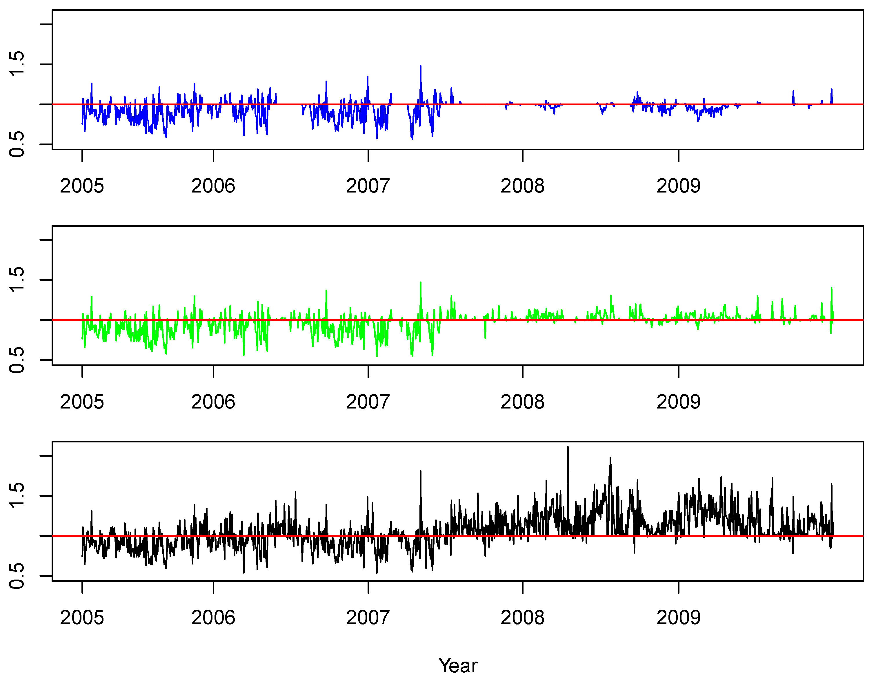
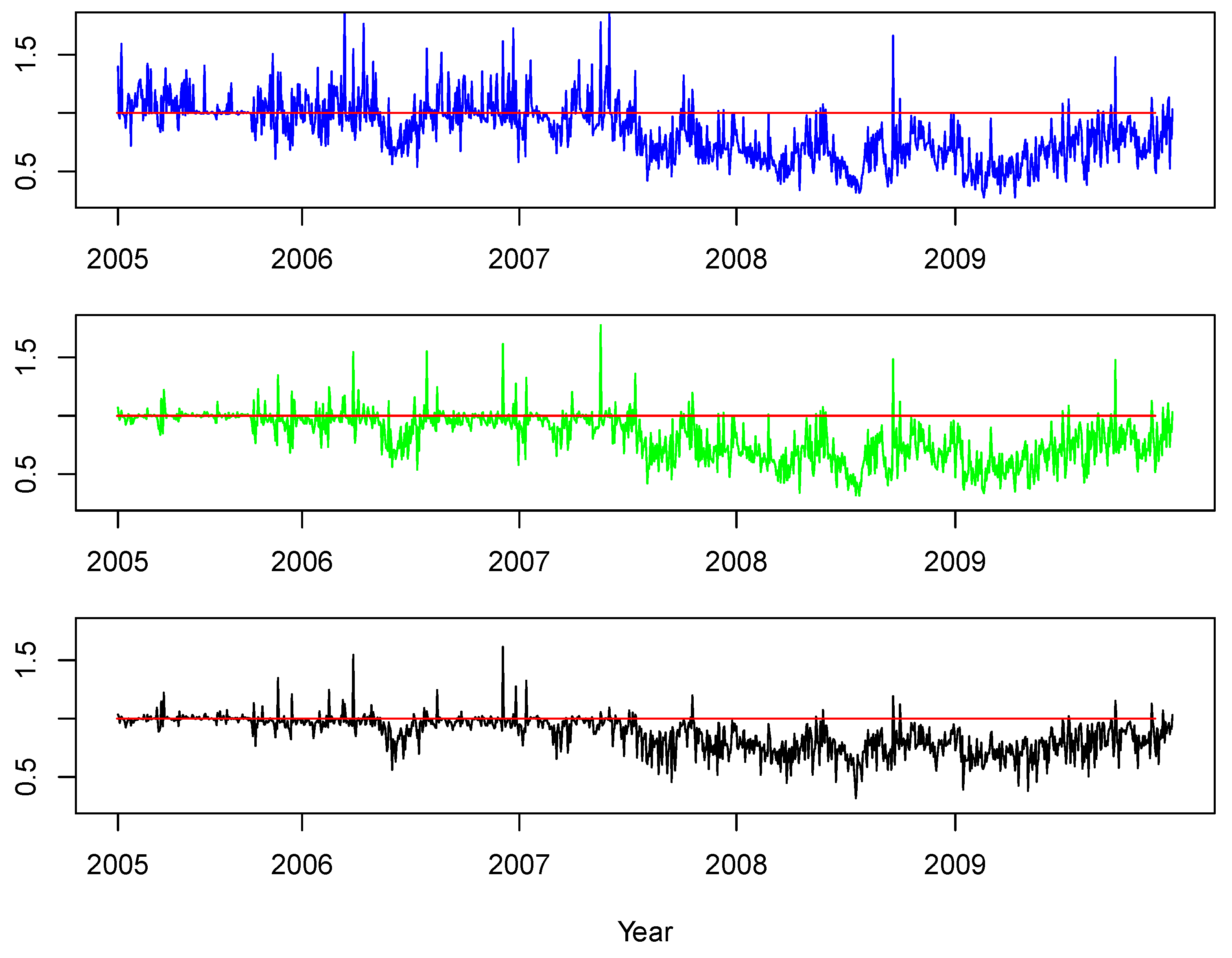
For a further illustration of our our results, we visualize the time series of portfolio variance ratios with respect to the benchmarks of $P_{\mathrm{low}}$ and $P_{ew}$. In particular, for the HAR, AR(5), and AR(1) approaches, we report the time series of ${\sigma }_t^2({\tilde{w}}_t,{\tilde{L}}_t)/{\sigma }_{\mathrm{low},t}^2$ and ${\sigma }_t^2({\tilde{w}}_t,{\tilde{L}}_t)/{\sigma }_{ew,t}^2$ in Figure 9 and Figure 10, respectively.

In Figure 9 for the benchmark $P_{\mathrm{low}}$, we observe that the HAR-based approach suggested to diversify only at a comparatively small number of days, whereas most of the time, the ratio was equal to one, i.e., no diversification was recommended. It provided the major correct recommendation before the start of the crisis. The AR(5) suggested very often diversification decisions; however, they appeared to be mostly disadvantageous from the start of the subprime mortgage crisis in the middle of 2007. The AR(1) model provided mostly wrong diversification decisions, especially during the crisis year 2008. Note that the reasons for these false recommendations could be attributed to either $L_t$ or $w_t$ forecasting models. Hence, it is apparent that AR(1) is not really suitable for our purposes here.

Different from the case above, in Figure 10, for the benchmark $P_{ew}$, we observe that the HAR model provided reasonable diversification recommendations especially since the crisis began in 2007; however, it was not really useful before the crisis start. Surprisingly, the other two approaches—AR(5) and AR(1)—also performed similarly to the HAR for this equally-weighted portfolio benchmark. We interpreted these findings as evidence that not only the choice of the time series model, but also the choice of the benchmark could determine the success of a portfolio diversification strategy.

5. Conclusions

The availability of intraday returns allows constructing precise realized volatility measures, which should be used for the improvement of risk management procedures. In this paper, we introduced the novel realized measure for portfolio diversification benefits. Our procedure would help to decide whether to include or not to include an additional security into the risky asset portfolio in order to reduce its variance.

After providing the asymptotic properties of our realized diversification measures, we considered several time series models for them such that we formulated a diversification decision rule. The performance of these models was evaluated in the empirical study based on a dataset of 10 risky assets. We found that the HAR time series approach was mostly suitable for out-of-sample prediction of realized diversification measures, as well as in order to forecast the optimal proportion of wealth to invest into the additional asset.

References

- Barndorff-Nielsen, Ole E., and Neil Shephard. 2004. Econometric analysis of realized covariation: High frequency based covariance, regression, and correlation in financial economics. Econometrica 72: 885–925. [Google Scholar] [CrossRef]
- Bera, Anil K., and Sung Y. Park. 2008. Optimal portfolio diversification using the maximum entropy principle. Econometric Reviews 27: 484–512. [Google Scholar] [CrossRef]
- Best, Michael J., and Robert. R. Grauer. 1991. On the sensitivity of mean-variance-efficient portfolios to changes in asset means: Some analytical and computational results. Review of Financial Studies 4: 315–42. [Google Scholar] [CrossRef]
- Brandt, Michael W., Pedro Santa-Clara, and Rossen Valkanov. 2009. Parametric portfolio policies: Exploiting characteristics in the cross-section of equity returns. Review of Financial Studies 22: 3411–47. [Google Scholar] [CrossRef]
- Callot, Laurent A., Anders B. Kock, and Marcelo C. Medeiros. 2017. Modeling and forecasting large realized covariance matrices and portfolio choice. Journal of Applied Econometrics 32: 140–58. [Google Scholar] [CrossRef]
- Chopra, Vijay K., and William T. Ziemba. 1993. The effects of errors in means, variances, and covariances on optimal portfolio choice. Journal of Portfolio Management 19: 6–11. [Google Scholar] [CrossRef]
- Choueifaty, Yves, and Yves Coignard. 2008. Toward maximum diversification. Journal of Portfolio Management 35: 40–51. [Google Scholar] [CrossRef]
- Corsi, Fulvio. 2009. A simple approximate long-memory model of realized volatility. Journal of Financial Econometrics 7: 174–96. [Google Scholar] [CrossRef]
- DeMiguel, Victor, Lorenzo Garlappi, Francisco J. Nogales, and Raman Uppal. 2009a. A generalized approach to portfolio optimization: Improving performance by constraining portfolio norms. Management Science 55: 798–812. [Google Scholar] [CrossRef]
- DeMiguel, Victor, Lorenzo Garlappi, and Raman Uppal. 2009b. Optimal versus naive diversification: How inefficient is the 1/N portfolio strategy? Review of Financial Studies 22: 1915–53. [Google Scholar] [CrossRef]
- Evans, John L., and Stephen H. Archer. 1968. Diversification and the reduction of dispersion: An empirical analysis. The Journal of Finance 23: 761–67. [Google Scholar]
- Frahm, Gabriel, and Christoph Memmel. 2010. Dominating estimators for minimum-variance portfolios. Journal of Econometrics 159: 289–302. [Google Scholar] [CrossRef] [Green Version]
- Frahm, Gabriel, and Christof Wiechers. 2013. A diversification measure for portfolios of risky assets. In Advances in Financial Risk Management. Edited by Jonathan A. Batten, Peter MacKay and Niklas Wagner. London: Palgrave Macmillan. [Google Scholar]
- Goetzmann, William N., and Alok Kumar. 2008. Equity portfolio diversification. Review of Finance 12: 433–63. [Google Scholar] [CrossRef]
- Golosnoy, Vasyl, and Yarema Okhrin. 2009. Flexible shrinkage in portfolio selection. Journal of Economic Dynamics and Control 33: 317–28. [Google Scholar] [CrossRef]
- Golosnoy, Vasyl, Wolfgang Schmid, Miriam I. Seifert, and Taras Lazariv. 2019. Statistical inferences for realized portfolio weights. Econometrics and Statistics 11. in press. [Google Scholar]
- Heber, Gerd, Asger Lunde, Neil Shephard, and Kevin K. Sheppard. 2009. Oxford-Man Institute’s Realized Library. version 0.2. Oxford: Oxford-Man Institute, University of Oxford. [Google Scholar]
- Jagannathan, Ravi, and Tongshu Ma. 2003. Risk reduction in large portfolios: Why imposing the wrong constraints helps. Journal of Finance 58: 1651–83. [Google Scholar] [CrossRef]
- Ledoit, Olivier, and Michael Wolf. 2003. Improved estimation of the covariance matrix of stock returns with an application to portfolio selection. Journal of Empirical Finance 10: 603–21. [Google Scholar] [CrossRef]
- Lütkepohl, Helmut. 2005. New Introduction to Multiple Time Series Analysis. Berlin/Heidelberg: Springer Science & Business Media. [Google Scholar]
- Lunde, Asger, Neil Shephard, and Kevin K. Sheppard. 2016. Econometric analysis of vast covariance matrices using composite realized kernels and their application to portfolio choice. Journal of Business & Economic Statistics 34: 504–18. [Google Scholar]
- Markowitz, Harry M. 1952. Portfolio selection. Journal of Finance 7: 77–91. [Google Scholar]
- Meucci, Attilio. 2009. Managing diversification. Risk 22: 74–79. [Google Scholar]
- Noureldin, Diaa, Neil Shephard, and Kevin K. Sheppard. 2012. Multivariate high-frequency-based volatility (heavy) models. Journal of Applied Econometrics 27: 907–33. [Google Scholar] [CrossRef]
- Rudin, Alexander M., and Jonathan S. Morgan. 2006. A portfolio diversification index. Journal of Portfolio Management 32: 81–89. [Google Scholar] [CrossRef]
Figure 1.
In-sample: autocorrelation functions of (left) and (right).
Figure 2.
Out-of-sample: autocorrelation functions of (left) and (right).
Figure 3.
, in-sample autocorrelations of HAR residuals (left) and their squares (right).
Figure 4.
, in-sample autocorrelations of AR(5) residuals (left) and their squares (right).
Figure 5.
, in-sample autocorrelations of AR(1) residuals (left) and their squares (right).
Figure 6.
Figure 7.
Figure 8.
Figure 9.
Ratios for the HAR, AR(5), and AR(1) models, from above to below. Note: the red lines correspond to a ratio of one, indicating equal variances.
Figure 10.