Global Asset Allocation Strategy Using a Hidden Markov Model

1
Department of Industrial Engineering, Yonsei University, Seoul 03722, Korea
2
School of Economics and Trade, Kyungpook National University, Daegu 41566, Korea
*
Author to whom correspondence should be addressed.
J. Risk Financial Manag. 2019, 12(4), 168; https://doi.org/10.3390/jrfm12040168
Submission received: 29 August 2019
/
Revised: 20 October 2019
/
Accepted: 2 November 2019
/
Published: 6 November 2019
(This article belongs to the Special Issue AI and Financial Markets)
Abstract
:This study uses the hidden Markov model (HMM) to identify the phases of individual assets and proposes an investment strategy using price trends effectively. We conducted empirical analysis for 15 years from January 2004 to December 2018 on universes of global assets divided into 10 classes and the more detailed 22 classes. Both universes have been shown to have superior performance in strategy using HMM in common. By examining the change in the weight of the portfolio, the weight change between the asset classes occurs dynamically. This shows that HMM increases the weight of stocks when stock price rises and increases the weight of bonds when stock price falls. As a result of analyzing the performance, it was shown that the HMM effectively reflects the asset selection effect in Jensen’s alpha, Fama’s Net Selectivity and Treynor-Mazuy model. In addition, the strategy of the HMM has positive gamma value even in the Treynor-Mazuy model. Ultimately, HMM is expected to enable stable management compared to existing momentum strategies by having asset selection effect and market forecasting ability.
1. Introduction
When it comes to asset allocation, it is a very important consideration to predict the price movement of the investment target. This move is also related to the phenomenon of price momentum. Using this price momentum phenomenon, investment strategies reflecting the price trend of assets have been developed. The method of using price momentum has performed well in the majority of the past market (Antonacci 2013). However, it has a disadvantage in that investment decisions are made after a certain period when price trend has passed. We expect that the artificial intelligence method, which has recently expanded its application in the financial market, will help this point. Freitas et al. (2009) showed that a prediction-based portfolio optimization model using neural networks can capture short investment opportunities and outperform the mean-variance model. They used neural networks to predict stock returns and employed predicted stock returns to compose the portfolio. Maknickienė (2014) found ensemble of Evolino-Recurrent Neural Network (RNN) is effective in portfolio management.
The purpose of this study is to investigate whether the use of the artificial intelligence method can improve portfolio performance empirically for global asset allocation. In this paper, we propose a method of asset allocation using the Hidden Markov Model (HMM). In addition, we examine whether asset selection through the HMM can yield significant excess returns. In this paper, the asset class is divided into four groups (stocks, bonds, real estate, and commodities) for empirical analysis. We used Exchange Traded Funds (ETFs) to allocate assets that have the effect of investing in real assets and in various sectors as well as indices. ETFs have the advantage of lower transaction cost and taxes (Poterba and Shoven 2002).
The purpose of this study is to demonstrate empirically that the investment using the HMM is superior to the existing investment method.
The composition of this paper is as follows. Section 2 discusses asset allocation, momentum investing and HMM. Section 3 describes the investment method using the HMM proposed in this paper. Section 4 analyzes the results of the portfolio and evaluates its usefulness. Finally, in Section 5, the conclusion and the remaining task are discussed.
2. Literature Review
2.1. Asset Allocation
Asset allocation is a series of processes that optimize the portfolio of risk assets. The purpose of asset allocation is to create an efficient portfolio through diversified investment based on Markowitz’s portfolio theory published in 1952 (Markowitz 1952).
Asset allocation has a significant impact on the performance of the portfolio and the use of exchange-traded fund (ETF) makes portfolio construction relatively easy. Since the ETF consists of securities that follow the index, it can achieve the effect of diversified investment. Miffre (2007) found that ETFs are effective in global asset allocation strategies.
The mean-variance portfolio or modern portfolio theory proposed by Markowitz pursues maximum returns under a given risk. The mean-variance portfolio provides a foundation of modern finance theory and has numerous extensions and applications (Yin and Zhou 2004). Optimal asset allocation across many assets is important and difficult. Simaan (1997) compared the mean-variance model with the mean absolute deviation model. Elliott et al. (2010) investigated a mean-variance portfolio selection problem under a Markovian regime-switching Black-Scholes-Merton economy.
One of the most frequently used by academics is the traditional 60/40 portfolio of stocks/bonds (Chaves et al. 2011; Asness et al. 2012). This portfolio invests 60% in stocks that are risky asset and 40% in bonds that are safe asset. Asness (1996) showed that the 60/40 portfolio outperformed the stock 100% portfolio.
Also, equal weighted portfolio (1/N), which invests the same weight in asset groups is often used. DeMiguel et al. (2007) found that equal weighted portfolio has a lower turnover, higher Sharpe index and higher return than the existing mean variance portfolio.
We compare the proposed strategy with the 60/40 portfolio and the equal weighted portfolio. In addition, this study constructs a portfolio using ETFs/ETNs that are effective in global asset allocation strategies.
2.2. Momentum Investing
The price momentum was first introduced by Jegadeesh and Titman (1993). Momentum means that the future returns of the winning stocks, which prices have risen for 3 to 12 months, are higher than the future returns of the loser stocks, which prices have fallen over the same period.
Momentum can be largely classified as time series momentum and cross-sectional momentum. Stocks with low return over the past period continue to fall in price, while stocks with high return continue to have cross-sectional momentum across the stock (Grinblatt and Moskowitz (2003); Chordia and Shivakumar (2006); Sadka (2006); Zhu and Zhou (2009); Novy-Marx (2012); Fama and French (2012)).
There are also time series momentum using only the past information of the asset. We analyze financial assets including stocks, bonds, futures, currencies, and derivatives, and show that trading strategies that use time series momentum based on past returns can be statistically significant (Moskowitz et al. 2012). This effect has been reported to be a common phenomenon not only in the US market, but also in the global equity markets (Asness et al. 2013).
Momentum investment strategy refers to a strategy that expects excess returns by buying stocks that had high yields in the past and selling stocks that had low ones. For this time-series momentum, historical data from individual assets are used to identify trends in assets at present and make investment decisions. In this study, we compare strategy using the most common method of time series momentum with strategy to identify current trends by applying the HMM, a method of machine learning.
2.3. Hidden Markov Model (HMM)
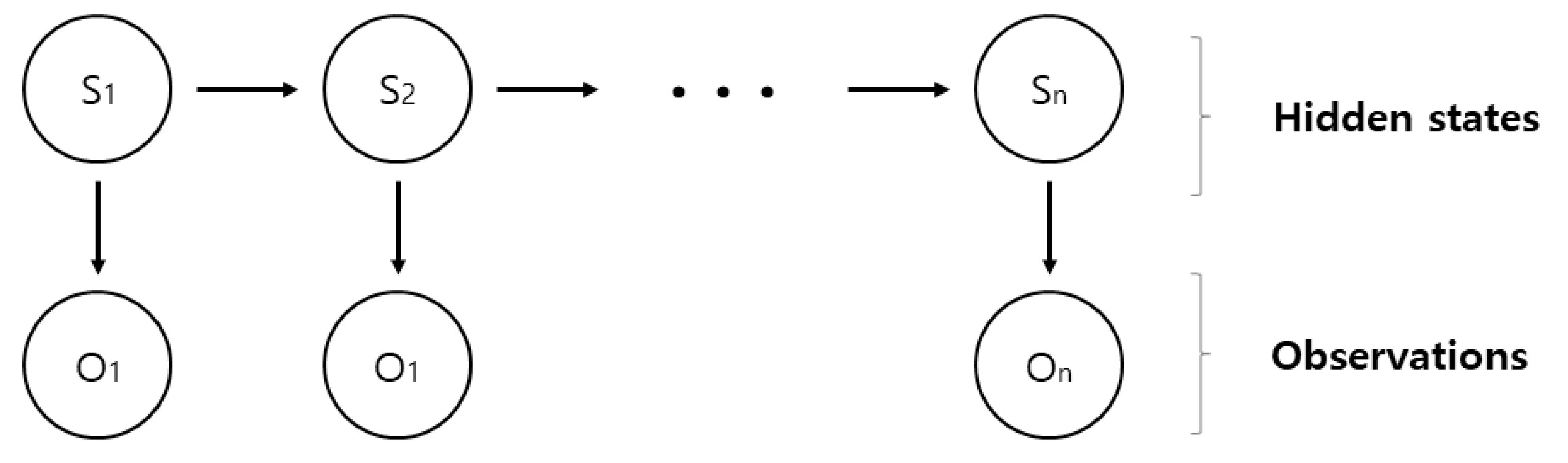
The HMM is a probability model that estimates the current state based on the assumption that the present state is only affected by the past state for sequential data. Importantly, it is assumed that each state in the HMM follows the Markov chain but is hidden. That is, as shown in Figure 1, the HMM is a model consisting of two hidden elements, a hidden state value (S) and an observable value (O) that actually allow movement between each component to follow the Markov chain. It is also composed of transition probability that connects hidden state to each hidden state. In order to estimate the HMM, there arises a problem of probability estimation, optimal state estimation, and model parameter estimation. Each problem is solved using a forward and backward algorithm, a Viterbi algorithm, and a Baum-Welch algorithm (Ramage 2007).
The HMM is mainly used for time series data and in the financial sector, it is widely used for the researches of the asset price prediction model and the transition of the asset. There is an empirical study that the stock price prediction using the HMM is meaningful (Hassan and Nath 2005). The HMM also approximates observations of asset prices into the Markov process to infer the current state of the asset which can help predict future asset prices using the current state and transition probability (Nguyen 2018). Kritzman et al. (2012) has shown that applying hidden state of the HMM to two cases, it is effective in exploring the phase change of market instability.
3. Model Specification
This study aims to comprehend phases of each assets and make portfolio by utilizing HMM. HMM can be used in case of situation that status variable cannot be figured out in advance. Figure 2 contains the overall process of analysis.
The return on each asset class ETF is used to learn the HMM and to identify the asset class regime through the distinct hidden states. Through the identified regime, we select the stocks to invest and finally construct the investment portfolio.
3.1. Data Source
To construct a portfolio model that compares with the HMM model used in this study, the price data of the ETF was used. A total of 23 ETFs representing each asset class were used for asset allocation. Since we assume monthly rebalancing, we calculated monthly returns and used adjusted stocks with adjusted dividends. The data source was used to invoke Yahoo Finance data using the “quantmod” package in the R program.
3.2. Learning of Hidden Markov Model
3.2.1. Markov Chain
The Hidden Markov model is based on the Markov chain. Markov chain refers to a discrete-time stochastic process with Markov properties. The key to the Markov chain is that the probability of one state depends only the state before it, and the transition from one state to another does not require a long history of state transition. It can be estimated as a transition from the last state.
3.2.2. Hidden Markov Model
The hidden Markov model represents a change in phenomena as a probabilistic model. It is assumed that each state follows a Markov chain but is hidden. The hidden Markov model is used to infer the indirectly hidden state using observations. The phases that can occur in the stock market are defined as the hidden states of the hidden Markov model, and the return of the asset class is used as input data. The model used in this study is as follows.
where is hidden Markov model, A = is transition matrix from i states to j states, B = is observation probability matrix where i states, is vector of initial probability of being in state and N is number of states.
Based on the input data, the hidden Markov model calculates the ‘state probability’ and the ‘transition probability’ for each hidden state. In this study, three hidden states are assumed. There are three problems to actually applying the hidden Markov model.
- (1)
- Estimate the probability of the observation(O) given the parameters of the hidden Markov model
- (2)
- Estimate the optimal state in that model given the observation(O)
- (3)
- Finally, only the most observation(O) problems in determining the optimal parameters of a hidden Markov model in a given state
The first and second problems can be solved with the dynamic algorithm based forward algorithm and the Viterbi algorithm, respectively. The third problem is solved with the Baum-Welch Algorithm. To use the hidden Markov model actually, we solved the above problems using the depmixS4 package of the R. The Observation data is asset price data. Each Model parameters can estimate Observation probability Matrix (B) on Hidden state and Transition Matrix (A).
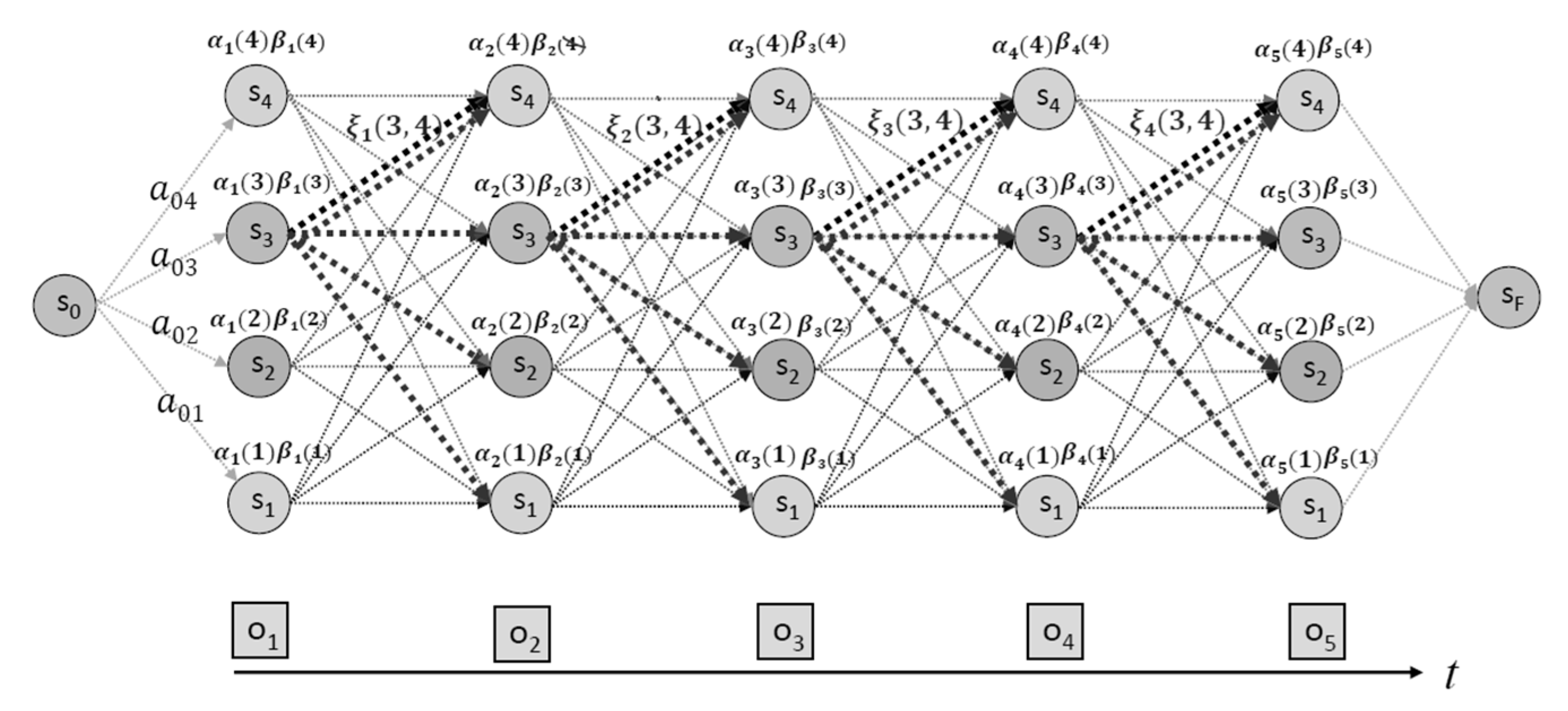
3.2.3. HMM Parameter Learning: Baum-Welch Algorithm
In this study, we used the Baum Welch algorithm (also called Forward, Backward Algorithm) to learn each parameter of the model to maximize the likelihood. The observation value O is a stock price data, and the parameters of each model may estimate the probability B Observation (O) can be observed in each hidden state and probability An Observation (O) can be shifted to another hidden state. Calculate the forward and backward probabilities respectively, based on the observation (O) with the parameters of the model, i.e., the fixed probability A and the emission probability B. Figure 3 illustrates the above process.
3.3. Estimation of Asset Phases & Portfolio Composition
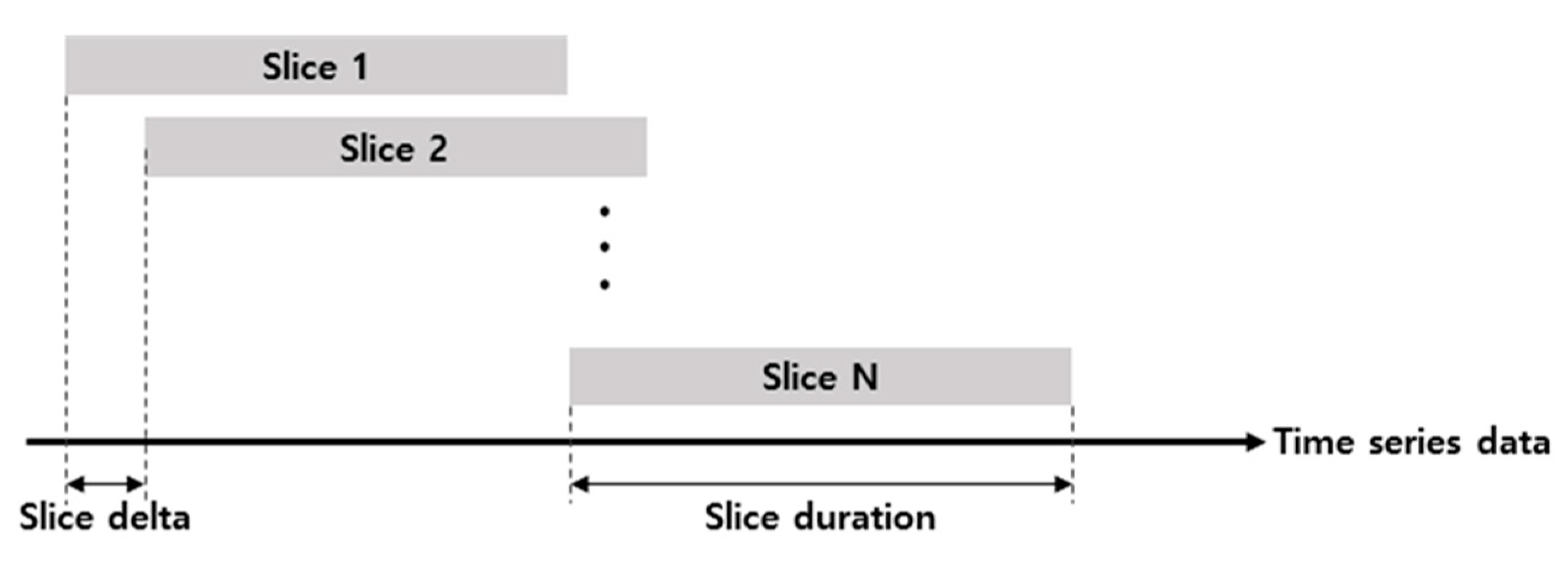
For analyzing Hidden states, compute average sharpe ratio on each state. If computed sharpe ratio is positive, we consider it increasing phases. We also trained HMM by using sliding window method which trains data of each asset for 2 years and replicates process of moving and training at intervals of one month. A schematic diagram of the sliding window method is shown in Figure 4. This methodology reflects decreasing of influence of previous data by not using all previous asset price data. It allows quicker adaptations to changing conditions on the market (Kaastra and Boyd 1996).
Each slice is trained by asset class using data from two years just before portfolio rebalancing. After learning, rebalancing is based on the results. In rebalancing, stock selection through HMM is as follows. In contrast, if sharpe ratio is negative, it might be decreasing phases. As a result, if Hidden state belonged to the present time has highest sharpe ratio, we consider the asset is in increasing phases. Assets selected by this process constitute a portfolio with equal weight.
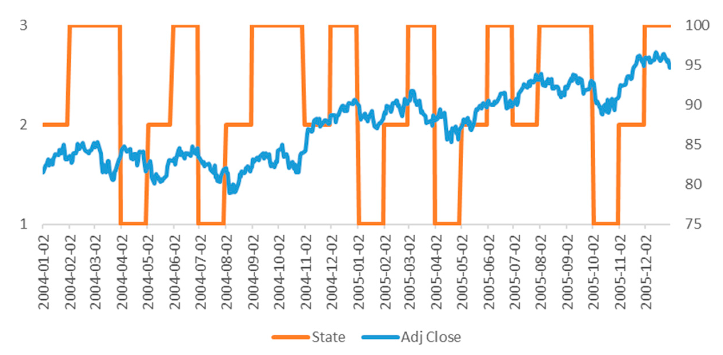
For comprehending overall process, we give an example. We apply SPY ETF adjusted close data to HMM from January 2004 to December 2005. Figure 5 contains division of hidden state by result of training.
In this time, we compute monthly average returns and sharp ratio for judging which phases by each hidden state. Looking at Table 1, in the state of 1, average monthly returns and sharp ratio is negative(−) and this can be considered decreasing phases. Also, in state 2, average monthly returns and sharpe ratio is positive and this can be considered increasing phases. In case of state 3, average monthly returns and sharp ratio is positive but it is not apparent compare to state 2. It might be considered stationary.
The latest date of Learning window, December 2005, cannot be included portfolio of next window, January 2006 because it’s not increasing phases. If sharpe ratio of input data is positive (+) and considered increasing phases, this asset can be included in portfolio. Assets selected by this process constitute a portfolio with equal weight.
3.4. Analyzing Effect of Asset Selection
In this study, various performance measures are used to verify the effectiveness of the proposed strategy. Through this, we understand why the performance of the proposed strategy is caused. Below are the major excess returns in this paper.
3.4.1. Information Ratio
The information rate is the ratio of the excess return resulting from active investment activity to the standard deviation of the return from active activity. Grinold and Kahn (1995), the basis of performance evaluation using information ratio, measured the information ratio using excess return and residual risk after considering systematic risk through regression analysis of benchmark return and portfolio return. It was argued that the magnitude of this value could determine the superiority of the performance.
where is return of portfolio, is the average return on the portfolio, Is the return on the benchmark, is the average return on the benchmark.
If IR is a positive value, it means that the manager valued the information and achieved the excess return, which is called the information rate because it shows the manager’s information capabilities.
3.4.2. Jensen’s Alpha
Jensen’s Alpha, also known as the Jensen’s Performance Index, is a measure of the excess returns earned by the portfolio compared to returns suggested by the CAPM model (Jensen 1968). The Jensen’s Alpha can be calculated by using following formula:
where is return of portfolio, is risk-free rate, is market return and is stock’s beta.
If Jensen’s alpha is positive which indicates over-performed the market on a risk-adjusted basis and ability of asset selection. In this study, we considered US Treasury bond (10-year) as risk-free rate.
3.4.3. Fama’s Net Selectivity
The Fama’s Net Selectivity Measure is suggesting a breakdown of portfolio performance (Fama 1972). It is given by the annualized return of the fund, deducted the yield of an investment without risk, minus the standardized expected market premium times the total risk of the portfolio under review. The Fama’s Net Selectivity can be calculated by using following formula:
where is return of portfolio, is risk-free rate, is market return, is the standard deviation of the portfolio return over period and is standard deviation of market return over period.
The Fama’s Net selectivity gives the excess return obtained by the manager that cannot have been obtained investing in the market portfolio. It compares the extra return obtained by the portfolio manager with a specific risk and the extra return that could have been obtained with the same amount of systematic risk.
3.4.4. Treynor-Mazuy Measure
In case of Jensen’s alpha, it cannot divide ability of asset selection and capture market timing. For analyzing in detail, we verify HMM asset allocation strategy by utilizing not only Jensen’s alpha also Treynor-Mazuy measure. The magnitude of the Treynor-Mazuy measure depends on two variables: the return of the fund and risk sensitivities variability. Treynor-Mazuy measure suggests that portfolios which display evidence of good market timing will be more volatile in up markets and less volatile in down markets (Treynor and Mazuy 1966). The Jensen’s alpha can be calculated by using following formula:
where is excess return of portfolio, is market premium, a is selectivity ability, is beta and is market timing performance.
If a portfolio has selectivity ability, a has a positive value and if a portfolio has market timing ability, has a positive value.
4. Empirical Analysis
HMM Strategy that we suggest in this study intends to capture each asset’s phases and constitute portfolio included stocks or assets having possibilities to increase. For empirical analysis, we apply our strategy to not only stock, bond but also alternative investment class like commodity and REIT’s. We constitute portfolio and make universe repetitively by sliding window methodology during January 2001–September 2019. In the above period, the HMM strategy was constructed by sliding 20 months of experiments, sliding for 1 month, sliding every month with 2 years of data. The investment period is January 2013–September 2019 excluding two years of initial learning.
4.1. Global Asset Allocation Investment Universe
In order to test robust of our strategy, we composed two universes. Table 2 and Table 3 contain the asset classes we used as universe. In order to obtain the closest effect to actual investment, we tested the ETF price following the asset class index. We set the cost of trading by assuming the median bid-ask spread of 0.10% applied to the turnover of the portfolio. So, a portfolio with higher turnover will greater trading costs. We set trading commissions to $0, assuming that investors are using a discount broker providing commission-free ETFs.
We further refined and tested the first 10 asset classes. In the case of alternative investments, we added some asset classes, as each asset class could not be further subdivided. Table 3 shows the investment universe with more granular asset classes.
4.2. Summary of Investment Result
We chose equal weighted portfolio, 60/40 portfolio, mean-variance portfolio, which is used for asset allocation as a benchmark for analyzing portfolio performance. In addition, by comparing the momentum strategy, we examine how the judgement of individual financial instrumental using HMM leads to investment performance.
In the EW portfolio, the asset classes that make up each universe were invested by 1/N. The share of stocks in an equal-weight portfolio will continue to change in proportion to returns. Therefore, we applied wall rebalancing to keep the equal weight. Also, for the 60/40 portfolio, the S & P 500 is 60% and 10-Year U.S. Treasury bond was composed of 40%. This proportion also continues to change with the returns on stocks and bonds. Therefore, in order to maintain a 60/40 fixed ratio, monthly rebalancing was applied. In the case of the MV portfolio, it means Markowitz’s mean-variance optimized portfolio, which has been optimized for weight with data from the past two years, which also applies monthly rebalancing. Lastly, the comparison MOM strategy selects positive stocks and excludes negative stocks based on 12-month momentum. Similarly, wall rebalancing was applied.
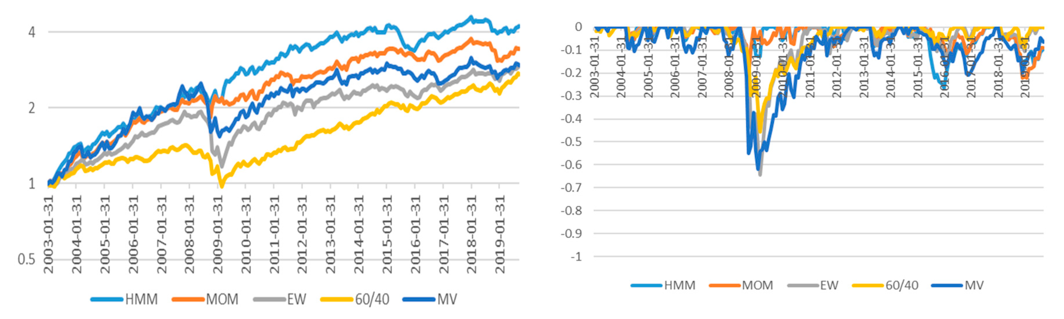
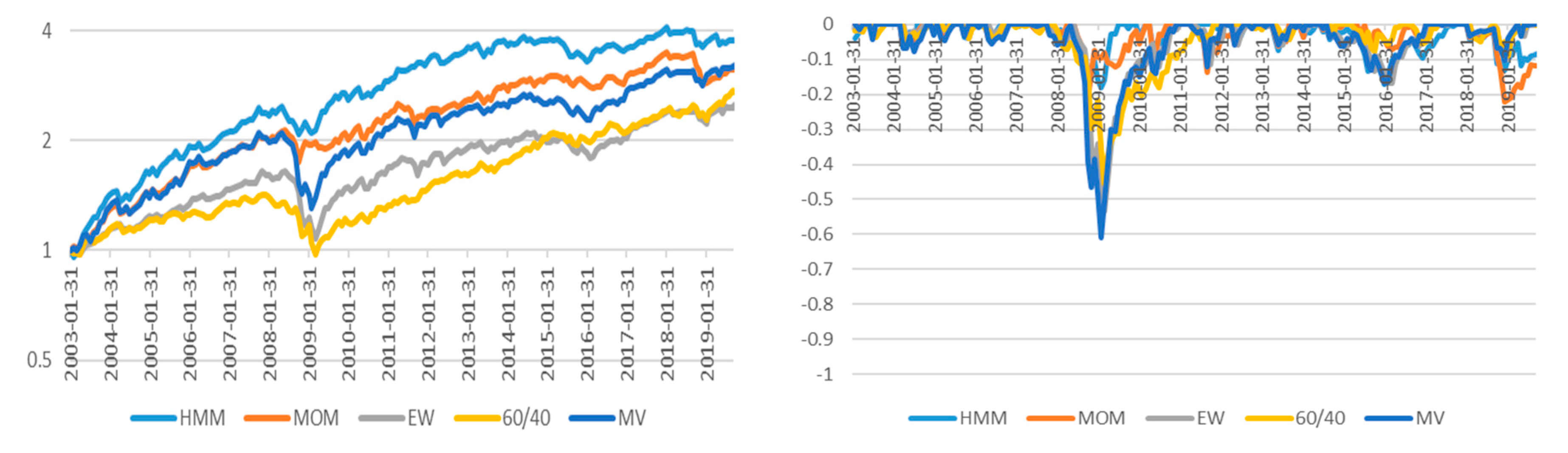
Figure 6 and Figure 7 show the cumulative portfolio returns and draw down charts for the two universes covered in this study. In both universes, the HMM strategy outperforms the momentum strategy. In the case of the draw down, it can be seen that the HMM and MOM strategies are superior to the traditional strategies used as benchmarks in this study. It’s remarkable that drawdown of HMM decreased while drawdown of benchmark increased in financial crisis time (2008). As a result, HMM stabilize risk of portfolio as well.
Table 4 summarizes the investment results. All of the strategies proposed in this study show that the investment performance is superior to the momentum strategy and benchmark. Also, universe 1 (Asset 10) and universe 2 (Asset 22) exhibit the same tendency. This implies that performance of the investment with HMM shows better investment performance than the strategy using classic asset allocation and momentum.
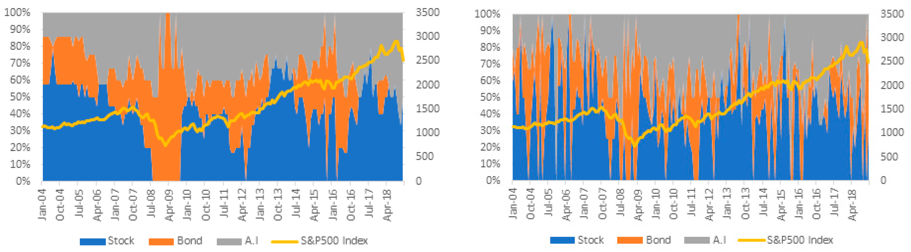
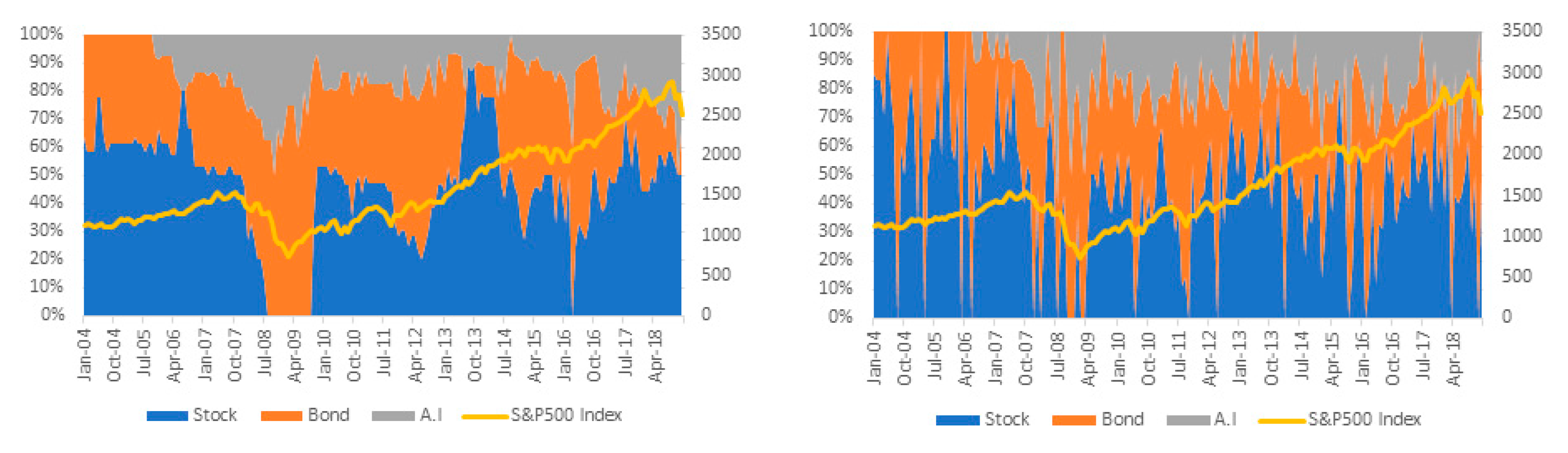
Figure 8 and Figure 9 are graphs showing the change in investment weight of strategy using momentum and HMM. The left side shows the momentum strategy and the right side shows the HMM strategy. Both strategies are defensive by increasing the weight of bonds in the 2008 financial crisis period. However, in the case of momentum, the weight of assets does not increase immediately after the index has bottomed out. This is because momentum is measured by a certain trend in the MOM strategy. In the case of HMM, on the other hand, it seems that the weight of bonds increases in the decline phases immediately and increase proportion of shares in the up phases. This shows that the strategy applying the HMM can figure out change of phases fast. This implies that the HMM strategy has a market timing capability compared to the MOM strategy.
Table 5 calculates the rolling return to calculate the probability that the strategy’s return outperforms each benchmark. Rolling returns are useful for examining the behavior of returns for holding periods, similar to those actually experienced by investors. The rolling period was examined from 1 month in the short term to 36 months in the long term. Overall, HMM strategy is more likely to outperform benchmarks than MOM strategies.
Information Ratio is widely used as an indicator for assessing performance in benchmarked funds, with the numerator in the form of fractions where the numerator is the excess return and the denominator is the standard deviation of the excess return. Table 6 summarizes the results of the information ratio. In this study, we set EW, 60/40, and MV portfolios as benchmarks. Therefore, when calculating the Information Ratio, each portfolio’s return was calculated as a benchmark.
4.3. Validation of Selection Effect of HMM
The tendency of the return distribution is highly related to the asset selection ability of the portfolio and market prediction ability. In this study, Jensen’s alpha, Fama’s Net Selectivity and Treynor-Mazuy are measured quantitatively. First, Table 7 shows the result of Jensen’s alpha for each universe. The benchmarks used the measure Jensen’s alpha were an equal weighted portfolio, 60/40 portfolio and mean-variance portfolio of assets that belonged to each universe. In both universes, we can see that Jensen’s alpha of HMM is about 2% larger than the momentum strategy. This tendency is the same for the EW portfolio, 60/40 portfolio and MV portfolio as well. This shows that both strategies using HMM and momentum have the effect of financial instrument selection and the size of HMM strategy is larger than MOM strategy.
Table 8 summarizes Fama’s measures. This shows that both momentum and HMM strategies are positive when compared to each benchmark. Fama’s Net Selectivity, like Jensen’s Alpha, has a positive value if it has a positive value. The above results show that the HMM strategy is superior to all benchmarks over the existing MOM strategy. This is the same result as measuring the stock selection effect through Jensen’s alpha.
Next, we use Treynor-Mazuy model to examine financial instrument selection ability and market prediction ability. The benchmark likewise sets up the EW portfolios, 60/40 portfolios and MV portfolio belonging to each universe. Table 9 summarizes the Treynor-Mazuy Measure results. First of all, the alpha showing the ability to select a stock shows that both the HMM strategy and the MOM strategy have positive values. This is the same conclusion as the measurement of Jensen’s alpha or Fama’s Net Selectivity. Also, in the case of gamma, which shows market timing capability, all of HMM strategies are positive, and some of them are negative in MOM strategy. If gamma is positive, market timing capability exists. The magnitude of this value shows that the HMM strategy is superior to the MOM strategy.
5. Conclusions
The purpose of this study is to verify the effect of asset allocation through an artificial intelligence method. In particular, the HMM identifies the stages of individual financial product change and identifies the usefulness of the investment strategy. The concealment status in the HMM can provide insight into the current asset class. This works similarly to identify whether existing momentum strategies are up or down via price momentum. In this study, we proposed a strategy to include the portfolio if it can be determined that the current state derived from HMM is an upward phase, and to exclude it from the portfolio. For comparison, we discussed a momentum strategy that uses trends in the historical prices of individual financial instruments. The benchmarks include the EW portfolio, the 60/40 portfolio, and Markowitz’s MV portfolio, which are the most used asset allocation. In order to confirm the robustness of model, two investment universes were largely set up.
Looking at portfolio performance, the HMM and momentum strategies in both universes show better average annual returns and sharp ratios than traditional asset allocation methods. This suggests that the two strategies improved in the down market, such as the financial crisis, by reducing the max draw down. On the other hand, comparing the HMM strategy and the momentum strategy shows that the overall strategy of HMM is superior. Since this preponderance can only occur in certain intervals, we calculated the probability that the rolling returns of the two strategies could outperform the BM. As a result, in all cases, the HMM strategy is more likely to outperform the benchmark than the momentum strategy. It is also shown that as the holding period increases, the probability increases. This is common in both universes. This shows that the HMM strategy is relatively robust and can be useful in real investments.
In this study, we tried to find out where the cause of this achievement was. Three representative methods of measuring portfolio performance were used. First, we looked at excess returns through the Alpha of Jensen. As Jensen’s Alpha is positive for both the HMM and MOM strategies, it demonstrates its ability to select stocks. Next, we examined the ability to select stocks through the method of Fama’s Net Selectivity. This value is also positive, indicating that there is a stock selection effect. In both cases, since HMM is larger than MOM strategy, HMM strategy’s stock selection ability is excellent. Finally, the strategy was evaluated using the Treynor-Mazuy model. The alpha of Treynor-Mazuy model shows the effect of stock selection, and the result is the same. Also, the value of gamma is the market timing capability, which also shows that the HMM strategy is larger than the MOM strategy.
Summarizing the above results, we can see that the MOM strategy and the HMM strategy are superior to the traditional portfolio composition strategy in terms of performance. This is because the HMM strategy and the momentum strategy, as discussed in this study, have a greater selection effect than the traditional strategy. In particular, the HMM strategy is more effective than the MOM strategy that managers use a lot.
The implications of this study are as follows. MOM strategy the invest in each financial instrument trend are well known and used frequently. MOM strategy has a process of identifying trends in the past through price data and investing in them. The HMM strategy shows that the investment result are superior to the MOM strategy by identifying trends in the financial instruments. Therefore, this method can be applied to bond portfolio, asset allocation portfolio as well as equity portfolio widely.
It is meaningful that this process has been identified through the HMM which is an Artificial Intelligence method. This indicates that an Artificial Intelligence can improve performance more than traditional investment methods. Therefore, further research needs to be applied to asset allocation strategies using deep learning such as RNN.
The limitations and future challenges of this study are as follows. First, in this study, we judged the phases by learning the returns of individual assets. However, as macroeconomic variable also influences the return of individual stocks and assets, these factors need to be considered as well. Second, investment decisions were made on a monthly basis. There is also a price trend on intraday, so it can be applied to high frequency areas as well.
Author Contributions
All the authors made important contribution to this paper. Conceptualization, E.-c.K.; Methodology, E.-c.K.; Software, E.-c.K. and H.-w.J.; Validation, H.-w.J. and N.-y.L.; Formal Analysis, E.-c.K. and N.-y.L.; Investigation, N.-y.L. and H.-w.J.; Resources, E.-c.K. and H.-w.J.; Data Curation, H.-w.J.; Writing-Original Draft Preparation, E.-c.K. and N.-y.L.; Writing-Review & Editing, H.-w.J.; Visualization, N.-y.L.; Supervision, E.-c.K.
Funding
This research received no external funding.
Acknowledgments
We would like to thank the three anonymous reviewers who carefully reviewed our paper and provided us with intuitive suggestions and constructive comment. We are grateful to the editors for theirs support and effort for our manuscript.
Conflicts of Interest
The authors declare no conflict of interest.
References
- Antonacci, Gary. 2013. Absolute momentum: A simple rule-based strategy and universal trend-following overlay. SSRN Electronic Journal. [Google Scholar] [CrossRef]
- Asness, Clifford S. 1996. Why not 100% equities. Journal of Portfolio Management 22: 29. [Google Scholar] [CrossRef]
- Asness, Clifford S., Andrea Frazzini, and Lasse H. Pedersen. 2012. Leverage aversion and risk parity. Financial Analysts Journal 68: 47–59. [Google Scholar] [CrossRef]
- Asness, Clifford S., Tobias J. Moskowitz, and Lasse Heje Pedersen. 2013. Value and momentum everywhere. Journal of Finance 58: 929–86. [Google Scholar] [CrossRef]
- Chaves, Denis, Jason Hsu, Feifei Li, and Omid Shakernia. 2011. Risk parity portfolio vs. other asset allocation heuristic portfolios. The Journal of Investing 20: 108–18. [Google Scholar] [CrossRef]
- Chordia, Tarun, and Lakshmanan Shivakumar. 2006. Earnings and price momentum. Journal of Financial Economics 80: 627–56. [Google Scholar] [CrossRef]
- DeMiguel, Victor, Lorenzo Garlappi, and Raman Uppal. 2007. Optimal versus naive diversification: How inefficient is the 1/N portfolio strategy? The Review of Financial Studies 22: 1915–53. [Google Scholar] [CrossRef]
- Elliott, Robert J., Tak Kuen Siu, and Alex Badescu. 2010. On mean-variance portfolio selection under a hidden Markovian regime-switching model. Economic Modelling 27: 678–86. [Google Scholar] [CrossRef]
- Fama, Eugene. 1972. Components of Investment Performance. Journal of Finance 27: 551–67. [Google Scholar]
- Fama, Eugene F., and Kenneth R. French. 2012. Size, value, and momentum in international stock returns. Journal of Financial Economics 105: 457–72. [Google Scholar] [CrossRef]
- Freitas, Fabio D., Alberto F. De Souza, and Ailson R. de Almeida. 2009. Prediction-based portfolio optimization model using neural networks. Neurocomputing 72: 2155–70. [Google Scholar] [CrossRef]
- Grinblatt, Mark, and Tobias J. Moskowitz. 2003. Predicting stock price movements from the pattern of past returns. Journal of Financial Economics. [Google Scholar] [CrossRef]
- Grinold, Richard C., and Ronald N. Kahn. 1995. Active Portfolio Management: Quantitative Theory and Applications. Chicago: Probus. [Google Scholar]
- Hassan, Md Rafiul, and Baikunth Nath. 2005. Stock Market Forecasting Using Hidden Markov Models, A New approach. Paper presented at 5th International Conference on Intelligent Systems Design and Applications (ISDA’05), Warsaw, Poland, September 8–10. [Google Scholar]
- Jegadeesh, Narasimhan, and Sheridan Titman. 1993. Returns to buying winners and selling losers: Implications for stock market efficiency. The Journal of Finance 48: 65–91. [Google Scholar] [CrossRef]
- Jensen, Michael C. 1968. The Performance of Mutual Funds in the Period 1945–1964. The Journal of Finance 23: 389–416. [Google Scholar] [CrossRef]
- Kaastra, Iebeling, and Milton Boyd. 1996. Designing a neural network for forecasting financial and economic time series. Neurocomputing 10: 215–36. [Google Scholar] [CrossRef]
- Kritzman, Mark, Sebastien Page, and David Turkington. 2012. Regime Shifts: Implications for Dynamic Strategies. Financial Analysts Journal 68: 22–39. [Google Scholar] [CrossRef]
- Maknickienė, Nijole. 2014. Selection of orthogonal investment portfolio using Evolino RNN trading model. Procedia-Social and Behavioral Sciences 110: 1158–65. [Google Scholar] [CrossRef]
- Markowitz, Harry. 1952. Portfolio Selection. The Journal of Finance 7: 77–91. [Google Scholar]
- Miffre, Joëlle. 2007. Country-specific ETFs: An efficient approach to global asset allocation. Journal of Asset Management 8: 112–22. [Google Scholar] [CrossRef]
- Moskowitz, Tobias J., Yao Hua Ooi, and Lasse Heje Pedersen. 2012. Time series momentum. Journal of Financial Economics 104: 228–50. [Google Scholar] [CrossRef]
- Nguyen, Nguyet. 2018. Hidden Markov Model for Stock Trading. International Journal of Financial Studies 6: 36. [Google Scholar] [CrossRef]
- Novy-Marx, Robert. 2012. Is Momentum Really Momentum? Journal of Financial Economics 103: 429–53. [Google Scholar] [CrossRef]
- Poterba, James M., and John B. Shoven. 2002. Exchange-traded funds: A new investment option for taxable investors. American Economic Review 92: 422–7. [Google Scholar] [CrossRef]
- Ramage, Daniel. 2007. Hidden Markov Models Fundamentals. CS229 Section Notes 1. Available online: http://cs229.stanford.edu/section/cs229-hmm.pdf (accessed on 3 May 2019).
- Sadka, Ronnie. 2006. Momentum and post-earnings-announcement drift anomalies: The role of liquidity risk. Journal of Financial Economics 80: 309–49. [Google Scholar] [CrossRef]
- Simaan, Yusif. 1997. Estimation risk in portfolio selection: The mean variance model versus the mean absolute deviation model. Management Science 43: 1437–46. [Google Scholar] [CrossRef]
- Treynor, Jack L., and Kay K. Mazuy. 1966. Can Mutual Funds Outguess the Market? Harvard Business Review 44: 131–36. [Google Scholar]
- Yin, George, and Xun Yu Zhou. 2004. Markowitz’s mean-variance portfolio selection with regime switching: From discrete-time models to their continuous-time limits. IEEE Transactions on Automatic Control 49: 349–60. [Google Scholar] [CrossRef]
- Zhu, Yingzi, and Guofo Zhou. 2009. Technical analysis: An asset allocation perspective on the use of moving aveages. Journal of Financial Economics 92: 519–44. [Google Scholar] [CrossRef]
Figure 1.
Hidden Markov Model Trellis Diagram.

Figure 2.
Empirical Analysis Model Process.

Figure 3.
Forward Probability (α) & Backward Probability (β).

Figure 4.
Sliding Window Method.

Figure 5.
January 2004–December 2005 Optimal state of S&P500 Index.

Figure 6.
Portfolio Return and Drawdown Chart of Asset 10.

Figure 7.
Portfolio Return and Drawdown Chart of Asset 22.

Figure 8.
Change of Weights in Asset 10.

Figure 9.
Change of Weights in Asset 22.


Table 1.
Regime Detection by January 2004–December 2005 Optimal state of S&P500 Index.
| State | Average Monthly Return | Average Monthly Sharpe | Regime |
|---|---|---|---|
| 1 | −2.2572 | −0.6236 | Falling phase |
| 2 | 2.6337 | 0.9352 | Rising phase |
| 3 | 0.4293 | 0.1529 | Clearance phase |
Table 2.
Global Asset Allocation Invest Universe (Asset 10).
| Asset Class | Name | Following ETF/ETN Ticker |
|---|---|---|
| Stock | U.S Stock | SPY |
| Europe Stock | IEV | |
| Japan Stock | EWJ | |
| Emerging Market Stock | EEM | |
| Bond | Long-term U.S Treasury | TLT |
| Mid-term U.S Treasury | IEF | |
| Alternative investment | U.S REITs | IYR |
| Global REITs | RWX | |
| Gold | GLD | |
| Commodity | DBC |
Table 3.
Global Asset Allocation Invest Universe (Asset 22).
| Asset Class | Name | Following ETF/ETN Ticker |
|---|---|---|
| Stock | U.S Large Cap Stock | JKD |
| U.S. Small Cap Stock | IJR | |
| U.S Growth Stock | IVM | |
| Europe Stock | IEV | |
| Japan Stock | EWJ | |
| Korea Stock | EWY | |
| Developed Market Stock | EFA | |
| Emerging Market Stock | EEM | |
| Bond | Long-term U.S Treasury | TLT |
| Mid-term U.S Treasury | IEF | |
| U.S TIPS | TIP | |
| U.S Aggregate Bond | AGG | |
| Emerging Bond | EMB | |
| Global TIPS | GTIP | |
| High Yield Bond | HYT | |
| Alternative investment | U.S REITs | IYR |
| Global REITs | RWX | |
| Oil | OIL | |
| Gold | GLD | |
| Dollar | UUP | |
| Commodity | DBC | |
| Copper | CPER |
Table 4.
Portfolio Performance Summary.
| Name | Strategy | Benchmark | ||||
|---|---|---|---|---|---|---|
| HMM | MOM | EW | 60/40 | MV | ||
| Asset 10 | Ann Ret (Arith) | 0.0887 | 0.0781 | 0.0693 | 0.0623 | 0.0744 |
| Ann Ret (CAGR) | 0.0868 | 0.0756 | 0.0654 | 0.0605 | 0.0666 | |
| Ann Std Dev | 0.1027 | 0.0999 | 0.1064 | 0.0828 | 0.1382 | |
| Ann Sharp | 0.8449 | 0.7569 | 0.6148 | 0.7305 | 0.4822 | |
| Win Ratio | 0.6169 | 0.6219 | 0.6070 | 0.6468 | 0.5871 | |
| Maximum Draw Down | 0.2092 | 0.1819 | 0.3917 | 0.3138 | 0.3824 | |
| Asset 22 | Ann Ret (Arith) | 0.0811 | 0.0711 | 0.0578 | 0.0623 | 0.0748 |
| Ann Ret (CAGR) | 0.0799 | 0.0692 | 0.0548 | 0.0605 | 0.0709 | |
| Ann Std Dev | 0.0893 | 0.0898 | 0.0930 | 0.0828 | 0.1099 | |
| Ann Sharp | 0.8938 | 0.7704 | 0.5892 | 0.7305 | 0.6449 | |
| Win Ratio | 0.6517 | 0.6318 | 0.6318 | 0.6468 | 0.6318 | |
| Maximum Draw Down | 0.1612 | 0.1824 | 0.3488 | 0.3138 | 0.3789 | |
Table 5.
Portfolio Outperformance Probability.
| Strategy | HMM | MOM | |||||
|---|---|---|---|---|---|---|---|
| Benchmark | EW | 60/40 | MV | EW | 60/40 | MV | |
| Asset 10 | 1 months | 0.547 | 0.537 | 0.507 | 0.502 | 0.522 | 0.493 |
| 3 months | 0.508 | 0.598 | 0.528 | 0.492 | 0.523 | 0.487 | |
| 6 months | 0.531 | 0.602 | 0.520 | 0.515 | 0.551 | 0.526 | |
| 12 months | 0.611 | 0.674 | 0.600 | 0.574 | 0.579 | 0.505 | |
| 24 months | 0.680 | 0.629 | 0.635 | 0.573 | 0.545 | 0.573 | |
| 36 months | 0.729 | 0.572 | 0.711 | 0.633 | 0.446 | 0.669 | |
| Asset 22 | 1 months | 0.537 | 0.537 | 0.542 | 0.512 | 0.522 | 0.512 |
| 3 months | 0.558 | 0.593 | 0.518 | 0.543 | 0.503 | 0.497 | |
| 6 months | 0.571 | 0.617 | 0.561 | 0.546 | 0.551 | 0.531 | |
| 12 months | 0.584 | 0.611 | 0.579 | 0.658 | 0.584 | 0.505 | |
| 24 months | 0.697 | 0.573 | 0.708 | 0.635 | 0.545 | 0.494 | |
| 36 months | 0.723 | 0.524 | 0.747 | 0.717 | 0.470 | 0.608 | |
Table 6.
Information Ratio Result.
| Strategy | HMM | MOM | ||||
|---|---|---|---|---|---|---|
| Benchmark | EW | 60/40 | MV | EW | 60/40 | MV |
| Asset 10 | 0.2249 | 0.3002 | 0.3375 | 0.0867 | 0.1392 | 0.1671 |
| Asset 22 | 0.2928 | 0.2720 | 0.3213 | 0.1326 | 0.0989 | 0.0270 |
Table 7.
Jensen’s Alpha Result.
| Strategy | HMM | MOM | ||||
|---|---|---|---|---|---|---|
| Benchmark | EW | 60/40 | MV | EW | 60/40 | MV |
| Asset 10 | 0.0632 | 0.0593 | 0.0489 | 0.0489 | 0.0424 | 0.0270 |
| Asset 22 | 0.0565 | 0.0489 | 0.0348 | 0.0377 | 0.0301 | 0.0156 |
Table 8.
Fama’s Net Selectivity Result.
| Strategy | HMM | MOM | ||||
|---|---|---|---|---|---|---|
| Benchmark | EW | 60/40 | MV | EW | 60/40 | MV |
| Asset 10 | 0.0366 | 0.0247 | 0.0503 | 0.0178 | 0.0063 | 0.0312 |
| Asset 22 | 0.0402 | 0.0277 | 0.0356 | 0.0197 | 0.0071 | 0.0151 |
Table 9.
Treynor-Mazuy Measure Result.
| Strategy | HMM | MOM | |||||
|---|---|---|---|---|---|---|---|
| Benchmark | EW | 60/40 | MV | EW | 60/40 | MV | |
| Asset 10 | Alpha | 0.00697 | 0.00723 | 0.00427 | 0.00606 | 0.00682 | 0.00241 |
| Beta | −0.00444 | 0.0586 | 0.538 | −0.111 | −0.072 | 0.621 | |
| Gamma | 1.48 | 1.43 | 0.473 | 1.43 | 0.603 | 0.322 | |
| Asset 22 | Alpha | 0.00663 | 0.00695 | 0.00240 | 0.00537 | 0.00568 | 0.00288 |
| Beta | 0.0258 | 0.0776 | 0.651 | −0.034 | 0.0263 | 0.615 | |
| Gamma | 1.34 | 0.651 | 1.24 | 1.35 | 0.665 | −0.484 | |
© 2019 by the authors. Licensee MDPI, Basel, Switzerland. This article is an open access article distributed under the terms and conditions of the Creative Commons Attribution (CC BY) license (http://creativecommons.org/licenses/by/4.0/).
Share and Cite
MDPI and ACS Style
Kim, E.-c.; Jeong, H.-w.; Lee, N.-y. Global Asset Allocation Strategy Using a Hidden Markov Model. J. Risk Financial Manag. 2019, 12, 168. https://doi.org/10.3390/jrfm12040168
AMA Style
Kim E-c, Jeong H-w, Lee N-y. Global Asset Allocation Strategy Using a Hidden Markov Model. Journal of Risk and Financial Management. 2019; 12(4):168. https://doi.org/10.3390/jrfm12040168
Chicago/Turabian StyleKim, Eun-chong, Han-wook Jeong, and Nak-young Lee. 2019. "Global Asset Allocation Strategy Using a Hidden Markov Model" Journal of Risk and Financial Management 12, no. 4: 168. https://doi.org/10.3390/jrfm12040168