News-Driven Expectations and Volatility Clustering

Economic Science Institute, Chapman University, 1 University Drive, Orange, CA 92866, USA
J. Risk Financial Manag. 2020, 13(1), 17; https://doi.org/10.3390/jrfm13010017
Submission received: 27 December 2019
/
Revised: 14 January 2020
/
Accepted: 16 January 2020
/
Published: 20 January 2020
(This article belongs to the Special Issue LIQUIDITY: Efficiency and Stability in Financial Markets - Selected papers from 4th Chapman Conference on Money and Finance.)
Abstract
:Financial volatility obeys two fascinating empirical regularities that apply to various assets, on various markets, and on various time scales: it is fat-tailed (more precisely power-law distributed) and it tends to be clustered in time. Many interesting models have been proposed to account for these regularities, notably agent-based models, which mimic the two empirical laws through a complex mix of nonlinear mechanisms such as traders switching between trading strategies in highly nonlinear way. This paper explains the two regularities simply in terms of traders’ attitudes towards news, an explanation that follows from the very traditional dichotomy of financial market participants, investors versus speculators, whose behaviors are reduced to their simplest forms. Long-run investors’ valuations of an asset are assumed to follow a news-driven random walk, thus capturing the investors’ persistent, long memory of fundamental news. Short-term speculators’ anticipated returns, on the other hand, are assumed to follow a news-driven autoregressive process, capturing their shorter memory of fundamental news, and, by the same token, the feedback intrinsic to the short-sighted, trend-following (or herding) mindset of speculators. These simple, linear models of traders’ expectations explain the two financial regularities in a generic and robust way. Rational expectations, the dominant model of traders’ expectations, is not assumed here, owing to the famous no-speculation, no-trade results.

1. Introduction
A meticulous and extensive study of high-frequency financial data by various researchers reveals important empirical regularities. Financial volatility, in particular, obeys two well-established empirical laws that attracted special attention in the literature: it is fat-tailed (in fact power-law distributed with an exponent often close to 3) and it tends to be clustered in time, unfolding through intense bursts of high instability interrupting calmer periods (Mandelbrot 1963; Fama 1963; Ding et al. 1993; Gopikrishnan et al. 1998; Lux 1998; Plerou et al. 2006; Cont 2007; Bouchaud 2011). The first regularity implies that extreme price changes are much more likely than suggests the standard assumption of normal distribution. The second property, volatility clustering, reveals a nontrivial predictability in the return process, whose sign is uncorrelated but whose amplitude is long-range correlated. These are fascinating regularities that apply to various financial products (commodities, stocks, indices, exchange rates, Credit Default Swaps1) on various markets and on various time scales.
The universality and robustness of these laws (illustrated graphically in Section 2) suggests that there must be some basic, permanent, and general mechanisms causing them (an intuition that shall be the heuristic and guiding principle throughout this paper). To identify these causes requires going back to the basics of financial theory and contrasting the two major paradigms on financial fluctuations. The dominant view today, the efficient market hypothesis, treats an asset’s price as following a random walk exogenously driven by fundamental news (Bachelier 1900; Osborne 1959; Fama 1963; Cootner 1964; Fama 1965a, 1965b; Samuelson 1965; Malkiel and Fama 1970). On the other hand is the growing resurgence of an old view of financial markets that insists on endogenous amplifying feedback mechanisms caused by mimetic or trend-following speculative expectations, fueled by credit, and responsible for bubbles and crashes (Fisher 1933; Keynes 1936; Shiller 1980; Smith et al. 1988; Cutler et al. 1989; Orléan 1989; Cutler et al. 1990; Minsky 1992; Caginalp et al. 2000; Barberis and Thaler 2003; Porter and Smith 2003; Akerlof and Shiller 2009; Shaikh 2010; Bouchaud 2011; Dickhaut et al. 2012; Keen 2013; Palan 2013; Soros 2013; Gjerstad and Smith 2014; Soros 2015).2
The endogenous cause of financial volatility, probably predominant in empirical data (Bouchaud 2011), is particularly taken seriously in agent-based models, which, unlike neoclassical finance, deal explicitly with the traditional dichotomy of financial participants, investors versus speculators (often named differently), extending it to include other types of players; besides traders’ heterogeneity, these models also insist on traders’ learning, adaptation, interaction, etc. They generate realistic fat-tailed and clustered volatility, but typically through a complex mix of nonlinear mechanisms, notably traders’ switching between trading strategies. These interesting models of financial volatility have already been carefully reviewed elsewhere (Cont 2007; Samanidou et al. 2007; He et al. 2016; Lux and Alfarano 2016). The realism of these models comes at a price, however; it is not easy to isolate basic causes of the financial regularities amid a mathematically intractable complex of highly nonlinear processes at work simultaneously.3 While this literature contributed significantly to a faithful picture of financial markets, it is not completely satisfactory for a basic reason: the sophisticated trading behaviors commonly assumed in this literature, handled through modern computers, are hardly a natural explanation of the financial regularities, whose discovery (let alone validity) goes back to the 1960s, an early and more rudimentary stage of finance. There must be, in other words, something of a most fundamental nature, some permanent cause intrinsic to the very act of financial trading, that is causing these regularities. GARCH (generalized autoregressive conditional heteroskedasticity) models (Engle 1982; Bollerslev 1986; Bollerslev et al. 1992) are perhaps more popular and more parsimonious models of the two regularities than agent-based models; but these statistical models are hardly a theoretical explanation of the empirical laws from explicit economic mechanisms; when fitted to empirical data, moreover, they imply an infinite-variance return process, the integrated GARCH (or IGARCH) model (Engle and Bollerslev 1986), which corresponds to a more extreme randomness than the empirical one (Mikosch and Starica 2000, 2003).
This paper explains the two regularities simply in terms of traders’ attitudes towards news, an explanation that follows almost by definition of the traditional dichotomy of financial market participants, investors versus speculators, whose behaviors are reduced to their simplest forms. Long-run investors’ valuations of an asset are assumed to follow a news-driven random walk, thus capturing the investors’ persistent, long memory of fundamental news. Short-term speculators’ anticipated returns, on the other hand, are assumed to follow a news-driven autoregressive process, capturing their shorter memory of news, and, by the same token, the feedback intrinsic to their short-memory, trend-following (or herding) mindset. These simple, linear, models of traders’ expectations, it is shown below, explain the two financial regularities in a generic and robust way. Rational expectations, the dominant model of traders’ expectations, is not assumed here, owing to the famous no-speculation, no-trade results (Milgrom and Stokey 1982; Tirole 1982). In fact, there seems to be an intrinsic difficulty in building a realistic theory of high-frequency volatility of financial markets, caused by incessant trading at almost all time scales and often driven by short-term speculative gains, from rational expectations, since they typically lead to a no-speculation, no-trade equilibrium.
The model this paper suggests can be viewed as a simple theory of the interplay between the exogenous and endogenous causes of financial volatility that identifies the two components to be responsible for the two regularities, reducing them to basic, linear mechanisms; it is a synthesis of the two paradigms mentioned above, avoiding the caveats on both sides: the no-trade problem inherent to the neoclassical formulation of the news-driven random walk model, and the nonlinear complexity characteristic of agent-based models. The power-law tail of volatility can be shown to derive intrinsically from the self-reinforcing amplifications inherent to herding or trend-following speculative trading. Trend-following speculation, for example, which is a popular financial practice, leads directly to a random-coefficient autoregressive (RCAR) return process in a competitive financial market, assuming a simple linear competitive price adjustment, as recent empirical evidence suggests (Cont et al. 2014). The RCAR model derives naturally, provided that trend following is modeled, not in terms of moving averages of past prices (as often assumed in the agent-based literature) but in terms of moving averages of past returns, which is more natural and more convenient (Beekhuizen and Hallerbach 2017). The power-law tail of such processes is rigorously proven in the mathematical literature (Kesten 1973; Klüppelberg and Pergamenchtchikov 2004; Buraczewski et al. 2016).4 However, it can be proven that the RCAR model, briefly derived below (in Section 3)5, cannot explain volatility clustering, being a short-memory process (Mikosch and Starica 2000, 2003; Basrak et al. 2002; Buraczewski et al. 2016).6 The basic cause of clustered volatility, this paper suggests, is none other than the impact of exogenous news on expectations. A more general model is therefore suggested that includes, as usual, a second class of agents besides speculators: fundamental-value investors, who attach a real value to an asset and buy it when they think the asset is underpriced, or sell it, otherwise, updating additively their valuations with the advent of a fundamental, exogenous news; the amount of information a news reveal to the traders about the asset’s worth can be precisely quantified by the log-probability of the news, as is known from information theory (Shannon 1948). Speculators’ expectations are more subtle, since they are at least partly endogenous. The simplest compromise consists of modeling the speculators’ anticipated return as a first-order autoregressive process with a coefficient that is lower than 1, to capture speculative self-reinforcing feedback and shorter memory of fundamental news, but close enough to 1, so that the news have a persistent enough impact on speculators’ expectations as well. This extended model generates both the fat-tailed and clustered volatility.
2. The Empirical Regularities
Let be the price of a financial asset at the closing of period let the return (or relative price change) be The two empirical regularities read formally: (1) for big values where often being merely a normalizing constant); (2) over a long range of lags while for almost all Figure 1 and Figure 2 illustrate these two regularities for General Electric’s daily stock price and the New York Stock Exchange (NYSE) daily index7.
3. The Model
Following a traditional dichotomy, consider a financial market populated by two types of traders: (short-term) speculators, who buy an asset for anticipated capital gains; and (long-run fundamental-value) investors, who buy an asset based on its fundamental value. Let the (excess) demands of an investor and a speculator be respectively8:
where is a speculator’s estimation of the asset’s future price, is an investor’s estimation the asset’s present value, and the parameters Let and be, respectively, the numbers of investors and speculators active in period t. The overall (market) excess demand is:
where and are the average investor valuation (hereafter referred to simply as ‘the value’ of the security) and the average speculator anticipated future price.
Assume the following standard price adjustment, in accordance with the market microstructure literature9:
where is the overall market liquidity (or market depth) and Let the overall price impact of speculative and investment orders be denoted respectively as
The two Equations (3) and (4) combined yield:
3.1. A Purely News-Driven Investment Market Model
Let the arrival of exogenous news relevant to investors and speculators be modeled as random events and occurring with probability and leading the traders to additively revise their prior estimations of the asset by the amounts and respectively (which can be assumed normally distributed by aggregation). There is no harm in assuming namely a common access to the same news by all the traders. Thus the traders’ valuations of the asset follow a random walk: and where and are the indicator functions associated with the advent of the news. The amount of information the news reveals to the traders about the asset’s worth can be precisely quantified: and respectively. This news-driven random-walk of traders’ expectations should be distinguished from a standard assumption in the agent-based literature, introduced perhaps by Lux and Marchesi (1999), whereby an asset’s fundamental value is modeled as a noise-driven random walk, where the noise is a Gaussian white noise. The difference between a news and a noise is simple: a noise can be formally defined as a news that carries zero information 10
All in all, the asset’s price dynamics reads:
Because both types of traders are behaviorally equivalent, the investor-speculator dichotomy is of no substance in this specific model: is equivalent to and both are entirely driven by exogenous news. In other words, the market thus modeled is in fact a non-speculative purely news-driven market of investors. Figure 3 shows a simulation of this model, and Figure 4 shows five superposed sample paths of the model. All the parameter specifications are reported in Table 1 in Section 4. The clustering of volatility is generic in this model; but, as is clear from Figure 3, the model suffers from an obvious non-stationarity of the return process due to the double random walk of the traders’ expectations; thus the graphical impression of a robust fat tail is an artefact: it does not make sense to say that the distribution is fat-tailed (since the returns are in fact drawn from different distributions; for example, the standard deviation of the return varies greatly from sample to sample, as should be expected).
3.2. A Purely Speculative Trend-Following Market Model
Let the speculators’ anticipated return be denoted by:
Trend-following implies that speculators’ overall anticipated return is of the form where we have added the impact of exogenous news on speculators’ expectations. The weighting scheme can be computed explicitly from standard moving-average trend-following techniques used by financial practitioners (Beekhuizen and Hallerbach 2017). In a purely speculative market , the asset’s return is then This RCAR model generates, under quite general and mild technical conditions, a strictly stationary power law tail where the exponent depends solely on the joint distribution of and not on the exogenous news (Klüppelberg and Pergamenchtchikov 2004; Buraczewski et al. 2016). But this strict stationary property comes at a price, as noted in the introduction: for any such autoregressive model, and for any arbitrary function when it is well-defined, decays rapidly, at an exponential rate, with the lag (Mikosch and Starica 2000; Basrak et al. 2002). Thus, volatility cannot be long-range correlated in this purely speculative trend-following model, whether measured as or more generally by any function .
3.3. A More General Model
The two polar models emphasize a tension between the endogenous and the exogenous causes of volatility: the purely exogenous, news-driven, expectations, produces a clustering of volatility but induces a trivial non-stationarity; whereas the purely endogenous feedback-inducing trend-following expectations generates a stationary power-law tail but cannot account for volatility clustering. The simplest compromise between these two notions consists of maintaining a purely exogenous, news-driven investors’ valuations, but to assume that the speculators’ anticipated return is partly endogenous (self-referential, or reflexive) and to write where to capture the (exponentially decaying) short-memory of speculators’ concerning a fundamental news, but so that incoming news have a lasting enough impact upon the speculators’ expectations.11 The purely news-driven random walk of investors’ valuations, on the other hand, implies that the asset’s value incorporates all the fundamental news (news relevant to investors) in the sense that making the natural estimate of the asset’s fundamental value in this model.
All in all, the asset’s price dynamics in the general model reads:
4. Discussion
Both the fat tail and the volatility clustering are generic and robust in the model: they hold for a broad class of distributions and parameters. The specifications in Figure 3, Figure 4, Figure 5, Figure 6 and Figure 7 are chosen merely for illustration, except to reflect realistic orders of magnitude compared to empirical data (notably the standard deviation of return which is typically around 1). Also, in all the simulations: periods; and are independent identically distributed (IID) exponential processes; and are zero-mean Gaussian IID processes. The differing parameter choices are reported in Table 1.
5. Conclusions
This paper suggests a simple explanation for excess and clustered volatility in financial markets through a simple synthesis of the two major paradigms in financial theory. Excess volatility means that price fluctuations are too high given the underlying fundamentals, which is an intrinsic feature of the model, owing to the amplifying feedback intrinsic to speculative trading, as illustrated more strikingly in Figure 7, in which the fundamental value is kept constant. Clustered volatility simply reflects, in this theory, the traders’ persistent memory of exogenous news concerning the asset’s present value or future price: this persistent memory of news leads to persistent trade responses and persistent volatility. The two empirical facts are thus reduced to simple explanations, through basic linear processes.
Funding
This research received no external funding.
Acknowledgments
For helpful comments and suggestions, the author thanks V. L. Smith, C. Wihlborg, D.P. Porter, J.-P. Bouchaud, and two anonymous reviewers. The usual disclaimer applies.
Conflicts of Interest
The author declares no conflict of interest.
References
- Akerlof, George A., and Robert J. Shiller. 2009. Animal Spirits: How Human Psychology Drives the Economy, and why it Matters for Global Capitalism. Princeton: Princeton University Press. [Google Scholar]
- Aoki, Masanao. 2002. Open models of Share Markets with two Dominant Types of Participants. Journal of Economic Behavior & Organization 49: 199–216. [Google Scholar]
- Bachelier, Louis. 1900. Theory of Speculation. In The Random Character of Stock Market Prices. Edited by Paul H. Cootner. Cambridge: MIT Press. (In French) [Google Scholar]
- Barberis, Nicholas, and Richard Thaler. 2003. A Survey of Behavioral Finance. Handbook of the Economics of Finance 1: 1053–128. [Google Scholar]
- Basrak, Bojan, Richard A. Davis, and Thomas Mikosch. 2002. Regular Variation of GARCH Processes. Stochastic Processes and their Applications 99: 95–115. [Google Scholar] [CrossRef] [Green Version]
- Beekhuizen, Paul, and Winfried G. Hallerbach. 2017. Uncovering Trend Rules. The Journal of Alternative Investments 20: 28–38. [Google Scholar] [CrossRef] [Green Version]
- Bollerslev, Tim. 1986. Generalized Autoregressive Conditional Heteroskedasticity. Journal of Econometrics 31: 307–27. [Google Scholar] [CrossRef] [Green Version]
- Bollerslev, Tim, Ray Y. Chou, and Kenneth F. Kroner. 1992. ARCH Modeling in Finance: A Review of the Theory and Empirical Evidence. Journal of Econometrics 52: 5–59. [Google Scholar] [CrossRef]
- Bouchaud, Jean-Phillippe. 2010. Price Impact. In Encyclopedia of Quantitative Finance. Chichester: Wiley Online Library Press. [Google Scholar]
- Bouchaud, Jean-Philippe. 2011. The Endogenous Dynamics of Markets: Price Impact, Feedback Loops and IInstabilities. In Lessons from the Credit Crisis. London: Risk Publications, pp. 345–74. [Google Scholar]
- Bouchaud, Jean-Philippe, and Damien Challet. 2016. Why Have Asset Price Properties Changed so Little in 200 Years. In Econophysics and Sociophysics: Recent Progress and Future Directions. Cham: Springer, pp. 3–17. [Google Scholar]
- Buraczewski, Dariusz, Ewa Damek, and Thomas Mikosch. 2016. Stochastic Models with Power-Law Tails. New York: Springer. [Google Scholar]
- Caginalp, Gunduz, David Porter, and Vernon L. Smith. 2000. Overreaction, Momentum, Liquidity, And Price Bubbles in Laboratory and Field Asset Markets. Journal of Psychology and Financial Markets 1: 24–48. [Google Scholar] [CrossRef]
- Carvalho, Rui. 2004. The Dynamics of the Linear Random Farmer Model. International Symposia in Economic Theory and Econometrics 14: 411–30. [Google Scholar]
- Clauset, Aaron, Cosma Rohilla Shalizi, and Mark E. J. Newman. 2009. Power-law distributions in empirical data. SIAM Review 51: 661–703. [Google Scholar] [CrossRef] [Green Version]
- Cont, Rama. 2007. Volatility Clustering In Financial Markets: Empirical Facts and Agent-Based Models. In Long Memory In Economics. Berlin and Heidelberg: Springer, pp. 289–309. [Google Scholar]
- Cont, Rama, Arseniy Kukanov, and Sasha Stoikov. 2014. The price impact of order book events. Journal of Financial Econometrics 12: 47–88. [Google Scholar] [CrossRef] [Green Version]
- Cootner, Paul. H. 1964. The Random Character of Stock Market Prices. Edited by Paul H. Cootner. Cambridge: MIT Press. [Google Scholar]
- Cutler, David M., James M. Poterba, and Lawrence H. Summers. 1989. What Moves Stock Prices? The Journal of Portfolio Management 15: 4–12. [Google Scholar] [CrossRef]
- Cutler, David M., James M. Poterba, and Lawrence H. Summers. 1990. Speculative Dynamics and The Role of Feedback Traders. The American Economic Review 80: 63–68. [Google Scholar]
- Dickhaut, John, Shengle Lin, David Porter, and Vernon Smith. 2012. Commodity Durability, Trader Specialization, and Market Performance. Proceedings of the National Academy of Sciences 109: 1425–30. [Google Scholar] [CrossRef] [PubMed] [Green Version]
- Ding, Zhuanxin, Clive W. J. Granger, and Robert F. Engle. 1993. A Long Memory Property of Stock Market Returns and a New Model. Journal of empirical finance 1: 83–106. [Google Scholar] [CrossRef]
- Engle, Robert F. 1982. Autoregressive Conditional Heteroscedasticity with Estimates of the Variance of United Kingdom Inflation. Econometrica 50: 987–1007. [Google Scholar] [CrossRef]
- Engle, Robert F., and Tim Bollerslev. 1986. Modelling the Persistence of Conditional Variances. Econometric Reviews 5: 1–50. [Google Scholar] [CrossRef]
- Fama, Eugene F. 1963. Mandelbrot and the Stable Paretian Hypothesis. Journal of Business 36: 420–29. [Google Scholar] [CrossRef] [Green Version]
- Fama, Eugene F. 1965a. The Behavior of Stock-Market Prices. Journal of Business 38: 34–105. [Google Scholar] [CrossRef]
- Fama, Eugene F. 1965b. Random Walks in Stock Market Prices. Financial Analysts Journal 21: 55–59. [Google Scholar] [CrossRef] [Green Version]
- Fisher, Irving. 1933. The debt-deflation theory of great depressions. Econometrica 1: 337–57. [Google Scholar] [CrossRef] [Green Version]
- Gabaix, Xavier. 2009. Power Laws in Economics and Finance. Annual Reviews of Economics 1: 255–94. [Google Scholar] [CrossRef] [Green Version]
- Gabaix, Xaiver. 2016. Power Laws in Economics: An Introduction. The Journal of Economic Perspectives 30: 185–205. [Google Scholar] [CrossRef] [Green Version]
- Gjerstad, Steven D., and Vernon L. Smith. 2014. Rethinking Housing Bubbles: The Role of Household and Bank Balance Sheets in Modeling Economic Cycles. New York: Cambridge University Press. [Google Scholar]
- Gopikrishnan, Parameswaran, Martin Meyer, L. Nunes Amaral, and H. Eugene Stanley. 1998. Inverse Cubic Law for the Distribution of Stock Price Variations. The European Physical Journal B-Condensed Matter and Complex Systems 3: 139–40. [Google Scholar] [CrossRef]
- He, Xue-Zhong, and Kai Li. 2012. Heterogeneous Beliefs and Adaptive Behaviour in A Continuous-Time Asset Price Model. Journal of Economic Dynamics and Control 36: 973–87. [Google Scholar] [CrossRef] [Green Version]
- He, Xue-Zhong, Kai Li, and Chuncheng Wang. 2016. Volatility Clustering: A Nonlinear Theoretical Approach. Journal of Economic Behavior & Organization 130: 274–97. [Google Scholar]
- Inoua, Sabiou M., and Vernon L. Smith. 2020. Classical Economics: Lost and Found. The Independent Review, to be appeared. [Google Scholar]
- Keen, Steve. 2013. A Monetary Minsky Model of the Great Moderation and the Great Recession. Journal of Economic Behavior & Organization 86: 221–35. [Google Scholar]
- Kesten, Harry. 1973. Random Difference Equations and Renewal Theory for Products of Random Matrices. Acta Mathematica 131: 207–48. [Google Scholar] [CrossRef]
- Keynes, John Maynard. 1936. The General Theory of Interest, Employment and Money. London: Macmillan. [Google Scholar]
- Klüppelberg, Claudia, and Serguei Pergamenchtchikov. 2004. The Tail of The Stationary Distribution of a Random Coefficient AR (q) model. Annals of Applied Probability 14: 971–1005. [Google Scholar] [CrossRef] [Green Version]
- Kyle, Albert S. 1985. Continuous Auctions and Insider Trading. Econometrica 53: 1315–35. [Google Scholar] [CrossRef] [Green Version]
- Lux, Thomas. 1998. The Socio-Economic Dynamics of Speculative Markets: Interacting Agents, Chaos, and the Fat Tails of Return Distributions. Journal of Economic Behavior & Organization 33: 143–65. [Google Scholar]
- Lux, Thomas, and Simone Alfarano. 2016. Financial Power Laws: Empirical Evidence, Models, and Mechanisms. Chaos, Solitons & Fractals 88: 3–18. [Google Scholar]
- Lux, Thomas, and Michele Marchesi. 1999. Scaling and Criticality in a Stochastic Multi-Agent Model of a Financial Market. Nature 397: 498–500. [Google Scholar] [CrossRef]
- Lux, Thomas, and Michele Marchesi. 2000. Volatility Clustering in Financial Markets: A Microsimulation of Interacting Agents. International Journal of Theoretical and Applied Finance 3: 675–702. [Google Scholar] [CrossRef]
- Lux, Thomas, and Didier Sornette. 2002. On Rational Bubbles and Fat Tails. Journal of Money, Credit, and Banking 34: 589–610. [Google Scholar] [CrossRef]
- Malkiel, Burton G., and Eugene F. Fama. 1970. Efficient Capital Markets: A Review of Theory and Empirical Work. The Journal of Finance 25: 383–417. [Google Scholar] [CrossRef]
- Mandelbrot, Benoit B. 1963. The Variation of Certain Speculative Prices. The Journal of Business 36: 394–419. [Google Scholar] [CrossRef]
- Mikosch, Thomas, and Catalin Starica. 2000. Limit Theory For The Sample Autocorrelations and Extremes of a GARCH (1, 1) process. Annals of Statistics 28: 1427–51. [Google Scholar]
- Mikosch, Thomas, and Catalin Starica. 2003. Long-Range Dependence Effects and ARCH Modeling. In Long–Range Dependence: Theory and Applications. Edited by Paul Doukhan, George Oppenheim and Murad Taqqu. Boston, Basel and Berlin: Birkhäuser, pp. 439–59. [Google Scholar]
- Milgrom, Paul, and Nancy Stokey. 1982. Information, Trade and Common Knowledge. Journal of Economic Theory 26: 17–27. [Google Scholar] [CrossRef]
- Minsky, Hyman P. 1992. The Financial Instability Hypothesis. Working Paper no. 74. Annandale-on-Hudson: The Levy Economics Institute. [Google Scholar]
- Newman, Mark E. J. 2005. Power Laws, Pareto Distributions and Zipf’s Law. Contemporary Physics 46: 323–51. [Google Scholar] [CrossRef] [Green Version]
- Orléan, André. 1989. Mimetic Contagion and Speculative Bubbles. Theory and Decision 27: 63–92. [Google Scholar] [CrossRef]
- Osborne, Maury F. M. 1959. Brownian Motion in the Stock Market. Operations Research 7: 145–73. [Google Scholar] [CrossRef]
- Palan, Stefan. 2013. A Review of Bubbles and Crashes in Experimental Asset Markets. Journal of Economic Surveys 27: 570–88. [Google Scholar] [CrossRef]
- Plerou, Vasiliki, Xavier Gabaix, H. Eugene Stanley, and Parameswaran Gopikrishnan. 2006. Institutional Investors and Stock Market Volatility. Quaterly Journal of Economics 2: 461–504. [Google Scholar]
- Porter, David P., and Vernon L. Smith. 2003. Stock Market Bubbles in the Laboratory. The Journal of Behavioral Finance 4: 7–20. [Google Scholar] [CrossRef]
- Samanidou, E., Elmar Zschischang, Dietrich Stauffer, and Thomas Lux. 2007. Agent-Based Models of Financial Markets. Reports on Progress in Physics 70: 409. [Google Scholar] [CrossRef] [Green Version]
- Samuelson, Paul. A. 1965. Proof that Properly Anticipated Prices Fluctuate Randomly. Industrial Management Review 6: 41–49. [Google Scholar]
- Sato, Aki-Hiro, and Hideki Takayasu. 1998. Dynamic Numerical Models of Stock Market Price: From Microscopic Determinism to Macroscopic Randomness. Physica A: Statistical Mechanics and its Applications 250: 231–52. [Google Scholar] [CrossRef]
- Shaikh, Anwar. 2010. Reflexivity, Path Dependence, and Disequilibrium Dynamics. Journal of Post Keynesian Economics 33: 3–16. [Google Scholar] [CrossRef]
- Shannon, Claude Elwood. 1948. A Mathematical Theory of Communication. Bell system Technical Journal 27: 379–423. [Google Scholar] [CrossRef] [Green Version]
- Shi, Yu, Qixuan Luo, and Handong Li. 2019. An Agent-Based Model of a Pricing Process with Power Law, Volatility Clustering, and Jumps. Complexity. [Google Scholar] [CrossRef]
- Shiller, Robert J. 1980. Do Stock Prices Move Too Much to Be Justified by Subsequent Changes in Dividends? Cambridge: National Bureau of Economic Research. [Google Scholar]
- Smith, Vernon L., Gerry L. Suchanek, and Arlington W. Williams. 1988. Bubbles, Crashes, and Endogenous Expectations in Experimental Spot Asset Markets. Econometrica 56: 1119–51. [Google Scholar] [CrossRef]
- Soros, George. 2013. Fallibility, Reflexivity, and the Human Uncertainty Principle. Journal of Economic Methodology 20: 309–29. [Google Scholar] [CrossRef] [Green Version]
- Soros, George. 2015. The Alchemy of Finance. Hoboken: John Wiley & Sons. [Google Scholar]
- Tirole, Jean. 1982. On the Possibility of Speculation under Rational Expectations. Econometrica 50: 1163–81. [Google Scholar] [CrossRef]
| 1 | See, e.g., Bouchaud and Challet (2016). |
| 2 | The nuance in this diverse literature on endogenous financial instability, already clearly articulated by the classical economists (Inoua and Smith 2020), lies perhaps in the nature of the ultimate destabilizing force that is specifically emphasized in each tradition, notably human psychology (Keynes and behavioral finance) or the easy bank-issued liquidity that backs or fuels the speculative euphoria, without which this latter would be of no significant, macroeconomic, harm (Fisher, Minsky, Kindleberger, etc., and the classical economists who preceded them). |
| 3 | Other types of models are also suggested for the power law more specifically; one of them, for example, relates the power law of return to the trades of very large institutional investors (Plerou et al. 2006). |
| 4 | Random-coefficient autoregressive (RCAR) processes are also known as Kesten processes, named after H. Kesten whose seminal theorem proves their power-law tail behavior. Kesten’s theorem was perhaps first used in finance to study GARCH processes, which are in fact also Kesten processes. ‘Rational bubbles’ can also be interpreted as first-order RCAR processes assuming a random discount factor (Lux and Sornette 2002); but this model generates a tail exponent smaller than 1. First-order RCAR processes have also been suggested as approximations to complex agent-based mechanisms (Sato and Takayasu 1998; Aoki 2002; Carvalho 2004). In this paper, however, a general RCAR return process holds directly in a competitive market of trend-following speculators. |
| 5 | A more detailed study of the power-law tail of volatility as it emerges from the RCAR model is the subject of a planned follow-up paper. |
| 6 | It may seem paradoxical that GARCH models, being also RCAR processes, could nonetheless generate clustered volatility; but this latter is in reality an ‘IGARCH effect’ (Mikosch and Starica 2000, 2003). It is more the persistence implied by the near-integration in fitted GARCH models that mimics the volatility clusters in these models. This near integration of fitted GARCH models resembles the near integration of speculators’ anticipated return in this paper’s model. |
| 7 | The linear fit is based on a maximum-likelihood algorithm developed by Clauset et al. (2009), which is an important reference for the statistical test of empirical power laws; the program codes are available at http://tuvalu.santafe.edu/~aaronc/powerlaws/. For an introduction to power laws more generally, see, for example, Newman (2005) and Gabaix (2009, 2016). |
| 8 | Because nonlinearity adds no further insight to this theory, we assume these standard linear supply and demand functions, which can be viewed as first-order linear approximations of more general functions; also, since financial supply and demand can be treated symmetrically (by treating supply formally as a negative demand), one can think directly in terms of a trader’s excess demand, which is a demand or a supply, depending on the sign. |
| 9 | The seminal work is Kyle (1985). A distinction may be in order here: a ‘price adjustment function’ models the overall price impact of the competition of buyers and sellers in a market; empirical evidence suggests it is linear in financial markets (Cont et al. 2014); a related but different concept is the ‘price impact’ of a trade or series of trades, which is typically a concave function of trade volume (Bouchaud 2010). The first concept is relevant for a theorist studying a market as a whole; the second, perhaps for a trader wishing to minimize the execution cost of a given trade volume. |
| 10 | We are grateful to a reviewer whose comment makes us aware of the need to emphasize explicitly the difference between a news and a noise. It is common in agent-based models to assume a Gaussian white noise in the fundamental-value dynamics, starting from Lux and Marchesi (1999), who, however, note that this (noise-driven) random walk in their model has nothing to do with the stylized facts. In fact, they assume the Gaussian white noise precisely so that none of the emergent financial regularities in their models can be attributed to this white noise: “In order to ensure that none of the typical characteristics of financial prices can be traced back to exogenous factors, we assume that the relative changes of [fundamental value] are Gaussian random variables.” (Lux and Marchesi 1999, p. 499). In fact, Lux and Marchesi (2000) show that the fat tail and volatility clustering in their model hold even when the fundamental value is constant. This is the case in this paper’s model as well, as emphasized below (Figure 7). The reviewer nonetheless suggests that the white-noise assumption, along with traders’ heterogeneity, may be responsible for clustered volatility in the agent-based model by He and Li (2012). |
| 11 | An arbitrarily general AR model is recently suggested by Shi et al. (2019), which replicates and studies in detail the robustness of an earlier working version of this paper’s model (titled ‘The Random Walk Behind Volatility Clustering, 2016’). However, the choice is crucial for volatility clustering. |
| 12 | For greater visibility, only the first 1000 periods out of 10,000 are shown in the subplots (a), (a′), (b), and (b′). |
Figure 1.
General Electric stock: (a) price; (b) return (in percent); (c) cumulative distribution of volatility in log-log scale, and a linear fit of the tail, with a slope close to 3; (d) autocorrelation function of return, which is almost zero at all lags, while that of volatility is nonzero over a long range of lags (a phenomenon known as volatility clustering).

Figure 2.
New York Stock Exchange (NYSE) composite daily index. (a) index; (b) return; (c) tail; (d) autocorrelation function of return and absolute return.
Figure 2.
New York Stock Exchange (NYSE) composite daily index. (a) index; (b) return; (c) tail; (d) autocorrelation function of return and absolute return.

Figure 3.
A purely news-driven market model: (a) price and value; (b) return; (c) tail; (d) autocorrelation function of return and absolute return.
Figure 3.
A purely news-driven market model: (a) price and value; (b) return; (c) tail; (d) autocorrelation function of return and absolute return.

Figure 4.
The purely news-driven market model: five simulations superposed: (a) price; (b) return; (c) tail; (d) autocorrelation function of return and absolute return.
Figure 4.
The purely news-driven market model: five simulations superposed: (a) price; (b) return; (c) tail; (d) autocorrelation function of return and absolute return.
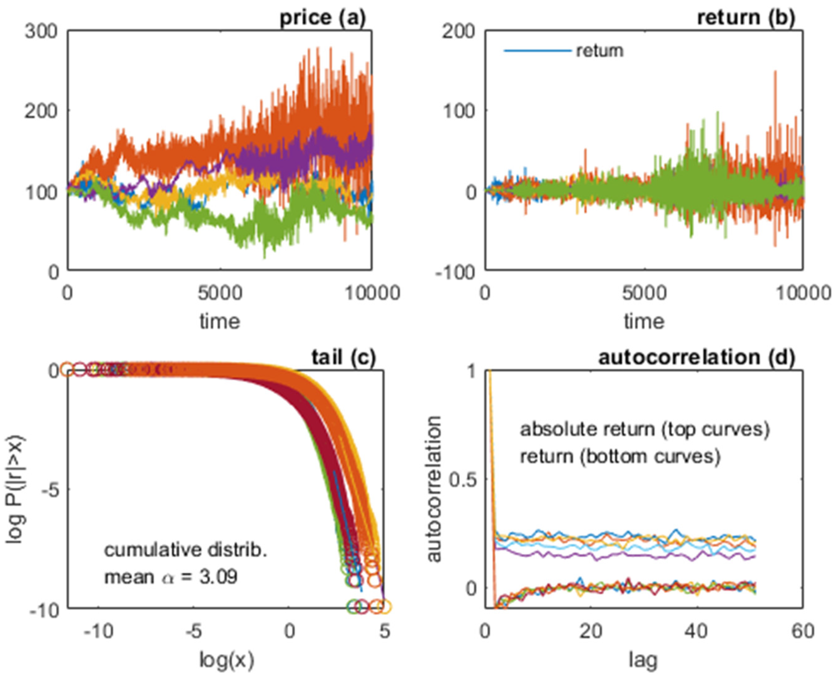
Figure 5.
The general model illustrated: (a) price and value; (b) return; (c) tail; (d) autocorrelation function of return and absolute return.
Figure 5.
The general model illustrated: (a) price and value; (b) return; (c) tail; (d) autocorrelation function of return and absolute return.

Figure 6.
The general model: five simulations superposed. (a) price; (b) return; (c) tail; (d) autocorrelation function of return and absolute return.
Figure 6.
The general model: five simulations superposed. (a) price; (b) return; (c) tail; (d) autocorrelation function of return and absolute return.

Figure 7.
The general model: variable versus constant fundamental value. (a,a′) price and value; (b,b′) return; (c,c′) tail; (d,d′) autocorrelation function of return and absolute return.12
Figure 7.
The general model: variable versus constant fundamental value. (a,a′) price and value; (b,b′) return; (c,c′) tail; (d,d′) autocorrelation function of return and absolute return.12


Table 1.
Parameter specifications.
| Figure 1 | Figure 2 | Figure 3 | Figure 41 | Figure 5 | Figure 61 | Figure 7 | |
|---|---|---|---|---|---|---|---|
| GE | NYSE | Model 1 | Model 1 | Model 2 | Model 2 | Model 2 | |
| Parameters | |||||||
| mean (m) | 0.1 | 0.1 | 0.2 | 0.2 | 0.2 | ||
| mean (n) | 0.1 | 0.1 | 0.1 | 0.1 | 0.1 | ||
| std () | 1 | 1 | 1 | 1 | 1 | ||
| std () | 1 | 1 | 0.04 | 0.04 | 0.04 | ||
| prob (News I) | 0.5 | 0.5 | 0.3 | 0.3 | 0.3 3; 0 4 | ||
| prob (News J) | 0.5 | 0.5 | 0.1 | 0.1 | 0.1 | ||
| a (feedback) | 0.99 | 0.99 | 0.99 | ||||
| mean (r) | −0.04 | −0.02 | 0.04 | 0.16 2 | 0.01 | 0.01 2 | 0.01 3; 0.01 3 |
| std (r) | 1.62 | 1.01 | 2.68 | 4.99 2 | 1.43 | 1.46 2 | 1.48 3; 1.44 3 |
1 Five sample paths superposed. 2 Average over five sample paths. 3 Left subplots (a)–(d). 4 Right subplots (a′)–(d′).
© 2020 by the author. Licensee MDPI, Basel, Switzerland. This article is an open access article distributed under the terms and conditions of the Creative Commons Attribution (CC BY) license (http://creativecommons.org/licenses/by/4.0/).
Share and Cite
MDPI and ACS Style
Inoua, S.M. News-Driven Expectations and Volatility Clustering. J. Risk Financial Manag. 2020, 13, 17. https://doi.org/10.3390/jrfm13010017
AMA Style
Inoua SM. News-Driven Expectations and Volatility Clustering. Journal of Risk and Financial Management. 2020; 13(1):17. https://doi.org/10.3390/jrfm13010017
Chicago/Turabian StyleInoua, Sabiou M. 2020. "News-Driven Expectations and Volatility Clustering" Journal of Risk and Financial Management 13, no. 1: 17. https://doi.org/10.3390/jrfm13010017