Models for Expected Returns with Statistical Factors

Abstract

In this paper, we propose multifactor models for the pan-European Equity Market using a block-bootstrap method and compare the results with those of traditional inferential techniques. The new factors are built from statistical measurements on stock prices—in particular, coefficient of variation, skewness, and kurtosis. Data come from Reuters, correspond to nearly 2000 EU companies, and span from January 2008 to February 2018. Regarding methodology, we propose a non-parametric resampling procedure that accounts for time dependency in order to test the validity of the model and the significance of the parameters involved. We compare our bootstrap-based inferential results with classical proposals (based on F-statistics). Methods under assessment are time-series regression, cross-sectional regression, and the Fama–MacBeth procedure. The main findings indicate that the two factors that better improve the Capital Asset Pricing Model with regard to the adjusted $R^2$ in the time-series regressions are the skewness and the coefficient of variation. For this reason, a model including those two factors together with the market is thoroughly studied. We also observe that our block-bootstrap methodology seems to be more conservative with the null of the GRS test than classical procedures.

1. Introduction

Understanding why and how certain assets go up in price while others go down is a major concern for both Industry and Academia. There is an overwhelming number of research articles regarding asset pricing; however, for the moment, no model has been able to explain the behaviour of the Stock Market in a fully satisfactory manner. Some of the classical proposed models rely on financial measures, such as the Price-to-Book ratio, Market Capitalisation, or Profitability to predict future asset returns (Fama and French 1992). Others also incorporate macro- or industry-related measures, such as interest rate levels (Viale et al. 2009), or oil price (Ramos et al. 2017). Another part of the literature focuses on higher order statistical moments of returns (Elyasiani et al. 2020). Lately, such measures are combined with others involving psychological factors, such as Momentum, in order to build more sophisticated models (Carhart 1997).

Markowitz (1952) determined that rational investors use diversification to optimize the profitability of their portfolios. This implies that the return required by an investor does not depend on the risk of a certain stock, because part of that risk is diversifiable. The only important factor is, thus, non-diversifiable risk. Markowitz assumes that investors are risk-averse, so when they choose a portfolio they tend to minimize the variance of the return of the portfolio for a given expected return and maximize the expected return for a given variance.

The Capital Asset Pricing Model, CAPM, (see Lintner 1965; Mossin 1966; Sharpe 1964) represents the expected profitability of the i-th stock, $E\left(R_i\right)$, in the following manner:

$$E\left(R_i\right)=r_f+{\beta }_i(E\left(r_m\right)-r_f),$$

where $r_f$ is the risk-free rate, $E\left(r_m\right)-r_f$ is the Market Risk Premium, and ${\beta }_i$ the sensitivity of expected excess asset’s return associated with the i-th asset.

CAPM is used to predict stock profitabilities, not portfolio profitabilities. According to Kristjanpoller and Liberona (2010), the best strategy under the assumptions of CAPM is a passive one: buy the Market portfolio in the long run. This conclusion is even stronger if we take into account transaction costs.

Even though CAPM is well-formulated on a theoretical level, the assumptions behind the model limit its practical application. For instance, CAPM’s $\beta$ is static and only applies for 1 year. Indeed, Lintner (1965) and Miller and Scholes (1972) tested the model with NYSE stocks obtaining certain inconsistencies, which led to the definition of multifactor models.

Multifactor models should better explain the behaviour of assets’ returns. The identification of these factors is a key issue in the process of building the model. The seminal example of multifactor models is the one by Fama and French (1992). The asset’s returns are explained by a linear model that depends on the size of the company (market capitalization), the price-to-book ratio, and, as in CAPM, the market risk premium:

$$E\left(R_i\right)=r_f+{\beta }_i(E\left(r_m\right)-r_f)+{\beta }_{i1}SMB+{\beta }_{i2}HML,$$

where $SMB$ is the difference between the return of a portfolio of small companies and one of big companies (small minus big), $HML$ is the difference between the return of a portfolio of companies with high price-to-book ratios and one of companies with low price-to-book ratios (high minus low), while $r_f$ and $E\left(r_m\right)$ are as before. Adding the two factors to the regressions results in large increases in the coefficient of determination. According to Fama and French (1993), the market factor alone produces only two (of 25) $R^2$ values greater than 0.9; in the three-factor regressions, $R^2$ values greater than 0.9 are usual (21 of 25).

Inferential procedures about multifactor models strongly rely on assumptions regarding the data: for instance, factors being uncorrelated over time, normally distributed errors which are i.i.d. over time and independent of the factors, and so forth. When these assumptions are not satisfied, classical estimators may be biased. To circumvent such a drawback, non-parametric techniques can be used.

Efron (1972) developed the Bootstrap methodology as a resampling technique to approximate the distribution of test statistics. In the Asset Pricing literature, Kosowski et al. (2006) proposed a bootstrap procedure by which they resample from the returns of mutual funds in order to test that all portfolios’ returns are explained by the factors. Fama and French (2010) modified the process to jointly resample both fund and explanatory returns. This additional step is important, as it takes into account possible correlation. However, none of these procedures consider dependency over time. Grané and Veiga (2008) explored the block bootstrap for computing the unconditional distribution of returns. These authors found huge differences in the minimum capital risk requirement estimates when using conditional approaches (such as GARCH-type models and stochastic volatility models) specially for long positions and larger investment horizons.

The objectives of this paper are: (1) to propose a multifactor model based on naive statistical factors, (2) develop non-parametric resampling techniques that account for time dependency in order to test the validity of the model and the significance of the parameters involved, and (3) to compare bootstrap-based inferential techniques with the classical proposals. These procedures are tested on a real dataset of assets’ returns of over 2000 European companies extracted from Reuters, and span from January 2008 to February 2018.

Specifically, the statistical factors that we consider are the coefficients of variation, skewness, and kurtosis of the stock prices. With the coefficient of variation, we aim to capture the stock volatility, while third- and fourth-order moments can also be strongly related to subsequent returns (see Chang et al. 2013; Conrad et al. 2013; Harvey and Siddique 2000). In the traditional framework, investors have specific preferences regarding the first (mean) and second (variance) moments of returns. Our intuition suggests that investors should also have preference for high-CV stocks or lottery stocks (Kumar 2009) and right-skewed portfolios (in fact, skewness could explain the excess returns found in portfolios of low-size and high book-to-markets in traditional models).

The main findings are that the two factors that better complement the market (only factor at the CAPM) are the skewness and the coefficient of variation. This is consistent with previous studies both for the US and the European markets that have found the existence of risk premia for volatility and skewness (Elyasiani et al. 2020). With regard to the time-series regressions, the conclusions drawn from the newly proposed bootstrap inferential techniques are somehow coherent with the ones obtained from classical inference procedures. Indeed, since the used data do not fulfill all the classical distributional requirements, the bootstrap conclusions tend to be less strict with departures from the benchmark described at the null hypotheses. In particular, our bootstrap inferences suggest that all adjusted time-series regression models have intercepts that are jointly equal to zero, which is not the case for the classical method. With respect to the specific models estimated for each portfolio, those with high loading on the coefficient of variation (respectively, skewness) have a higher coefficient of variation (resp. skewness) coefficient, while market $\beta$s are all close to $0.5$. The cross-section model built from the estimated coefficients presents some deficiency, since the coefficient of variation does not contribute significantly to it, while the market and skewness do. The underlying reason might be some multicollinearity problem. However, the performance of the model seems reasonably good in spite of the period analyzed, that comprises the European debt crisis.

The remainder of this paper is organized as follows. In Section 2 we present the materials and methods. Specifically, in Section 2.1 we discuss our data and the construction of portfolio returns, while Section 2.2 explains the methodology, first the classical (Time-Series, Cross-Sectional, and Fama-MacBeth) and second, the resampling technique developed for the analysis. Section 3 reports the results of the analysis and compares different methodologies. We close the paper with some conclusions in Section 4.

2. Materials & Methods

2.1. Data and Portfolio Returns

2.1.1. Data

We start with 2012 European companies that have been selected from all EU countries. We build up from the idea that a European multifactor asset pricing model exists and that its factors are equally priced across the European capital markets (Morelli 2010). As is usual in the Factor literature, we exclude Financials as they usually have high leverage ratios, affecting several financial ratios. We extract Reuters prices at the end of each month from January 2008 to February 2018 for these companies. We apply several filters to the data: first, we delete all the datapoints where price is not available; second, we apply a transaction filter, excluding all companies that do not show transactions for a whole semester; third, we exclude companies with no Market Cap or P/B info for more than two consecutive years. Finally, we exclude companies with non-positive equity at the end of any year. After all these filters have been passed, we end up with 1913 companies. Next, we calculate monthly returns for all the companies and estimate the Risk-Free Rate ($r_f$) with the two-year German Bond yield and Market ($r_m$) through the SP600. Monthly returns were calculated with the natural logs of the market price divided by the market price in the previous month.

Table 1. Descriptive statistics of the data by year.

Year	Companies	Months	Mean	SD	Min	Median	Max
2009	1631	12	69.55	1619.75	0.01	5.59	92,316.88
2010	1643	12	47.39	765.65	0.01	6.48	42,907.84
2011	1672	12	36.20	516.56	0.00	6.50	26,316.80
2012	1706	12	23.77	120.80	0.00	5.48	4203.77
2013	1729	12	24.98	109.47	0.00	5.98	3400.01
2014	1737	12	28.37	123.28	0.00	7.20	3789.00
2015	1789	12	30.98	139.74	0.00	7.25	3999.00
2016	1833	12	32.39	164.73	0.01	7.20	6000.00
2017	1864	12	38.99	195.06	0.00	8.74	6149.00
2018	1878	2	41.34	204.65	0.00	9.08	6000.00

contains some descriptive statistics by year. In particular, it provides the number of firms, the number of considered months in each period, and price statistics.

We can observe that the average price decreases until 2012 (from $69.55$ in 2009 to $23.77$ in 2012) and then increases until 2018 ($41.34$). This behaviour is related to the financial crisis. In terms of standard deviation, we can observe a similar pattern.

2.1.2. Statistical Factors

We calculated different measures for each stock in the sample, namely:

• Coefficient of variation (CV) of prices for each year and company:

  $$CV=\frac{s_n}{\overline{x}},$$

  where $s_n^2=\frac{1}{n}{\sum }_{i=1}^n{(x_i-\overline{x})}^2$ and $\overline{x}$ is the sample mean. CV represents the relative spread for positive random variables and it can take values in ($0,+\infty$).
• Skewness (Skew) of prices for each year and company:

  $$Skew=\frac{\frac{1}{n}{\sum }_{i=1}^n{(x_i-\overline{x})}^3}{s_n^3}$$
  Positive values indicate that the distribution is positively skewed, that is, the right tail is longer than the left one, while the contrary occurs for negative values. When both tails are similar, the skewness is roughly 0.
• Excess Kurtosis (Kurt) of prices for each year and company:

  $$Kurt=\frac{\frac{1}{n}{\sum }_{i=1}^n{(x_i-\overline{x})}^4}{s_n^4}-3$$

  measures how fat the tails of a distribution are in comparison to those of a normal random variable. Positive (negative) values indicate heavier (thinner) tails than those of a normal random variable.

In general, factors are positively correlated, except for Kurt, which is negatively correlated with Market and CV. As can be seen in

Table 2. Correlation among the factors.

	Market	CV	Kurt	Skew
Market	1.0000	0.5970	−0.4210	0.1770
CV	0.5970	1.0000	−0.5450	0.2930
Kurt	−0.4210	−0.5450	1.0000	0.1650
Skew	0.1770	0.2930	0.1650	1.0000

, Market and CV on one side and CV and Kurt on the other are highly correlated. This could lead to multicolineality in models built with these factors and, thus, to larger confidence intervals.

2.1.3. Portfolio Returns

Next, we calculate percentiles for each of these measures and assign them to portfolios accordingly following (Fama and French 1992). There are two portfolios for each measure, except for Skew, where we calculate three.

• Stocks with low CV will be included in portfolios 1-y-z, while stocks with high CV will be included in portfolios 2-y-z.
• Stocks with low Kurt will be included in portfolios x-1-z, while stocks with high Kurt will be included in portfolios x-2-z.
• Stocks with low Skew (less than the 30-th percentile, P30) will be included in portfolios x-y-1, while stocks with high Skew (greater than P70) will be included in portfolios x-y-3. The rest will be included in portfolios x-y-2.

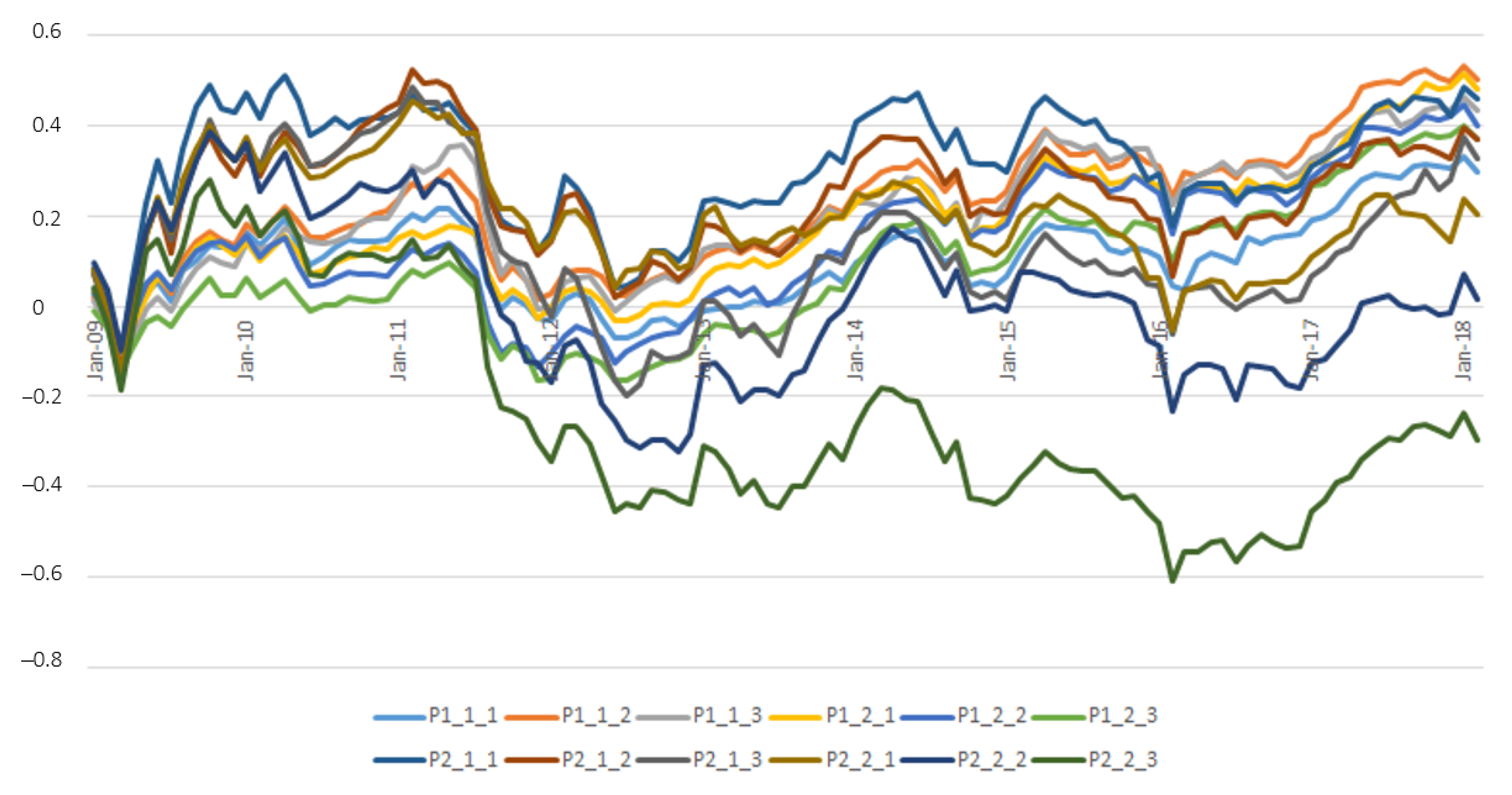
The resulting portfolios are summarized in

Table 3. Description of portfolios.

	Portfolio	CV	Kurt	Skew
(1)	1-1-1	Low	Low	Low
(2)	1-1-2	Low	Low	Medium
(3)	1-1-3	Low	Low	High
(4)	1-2-1	Low	High	Low
(5)	1-2-2	Low	High	Medium
(6)	1-2-3	Low	High	High
(7)	2-1-1	High	Low	Low
(8)	2-1-2	High	Low	Medium
(9)	2-1-3	High	Low	High
(10)	2-2-1	High	High	Low
(11)	2-2-2	High	High	Medium
(12)	2-2-3	High	High	High

. Portfolios are updated yearly based on the previous year’s measurements (2008 data are only used to build the starting portfolios). We proceed to calculate average monthly returns for the stocks included in each portfolio. Additionally, we calculate each factor as the excess return of the higher portfolio in each category minus the return of the lower portfolio. All returns are calculated for equally weighted portfolios at $t+1$. In Figure 1, we have plotted the cumulative returns of all the portfolios.

The three portfolios with the best performance are 1-1-2, 1-2-1, and 2-1-1. The first two share the feature of having low CV. There is one portfolio that ends with a negative cumulative return (2-2-3); it includes stocks with high CV, high Kurt, and high Skew. Portfolios 2-2-1 and 2-2-2 (high CV and high Kurt) are also among the worst performers.

2.2. Methodology

2.2.1. Classical Methodologies

Linear Factor Models have gained great popularity lately, and this has led to a vast amount of literature on estimating and testing such models. Typically, these models take the form of the following equation:

$$E\left(R_i\right)={\alpha }_i+{\beta }_i^{\prime }\lambda .$$

The expected return for the i-th portfolio has a linear relationship with a set of factors, $\lambda$. The simplest of such models is the one-factor model developed by Jensen (1968) and based on CAPM, where asset risk premiums are linear functions of market risk premium and the systematic risk of the asset (${\beta }_i$), that is:

$$E\left(R_i\right)={\alpha }_i+{\beta }_i(E\left(r_m\right)-r_f),$$

where $\alpha$ is referred to as the Jensen’s Alpha of the asset and is commonly used as a performance measure. In general, we will consider that a model works when the expected value of $\alpha$ is zero. The model is extendable, mainly, by including additional factors as independent variables. Feng et al. (2020) have made a great effort to systematically evaluate the contribution to asset pricing of any new factor, above and beyond what a high-dimensional set of existing factors explains.

Several procedures to estimate the parameters $\alpha$, $\beta$, and $\lambda$ have been developed in the literature. After reviewing two analytic procedures which assume a certain behaviour of the underlying data (Time-Series Regression and Cross-Sectional Regression), we propose a Block Bootstrap method that works even if the previous assumptions are violated.

The setup of the experiment includes N assets (portfolios of equities), K factors ($K=1$ for CAPM), and T time periods. The factors are excess returns. We use portfolios instead of stocks because: (1) the errors of $\alpha$ and $\beta$ are higher for individual stocks as their volatility is higher, and (2) portfolios have more stable characteristics, while stocks vary over time. All the statistics below are derived from the classical assumptions that returns are independent over time, correlated across assets, and (for finite sample results) normally distributed.

Time-Series Regression (TS)

A time-series regression was run for each portfolio $i=1,\dots ,N$ as

$$R_t^i={\alpha }_i+{\beta }_i^{\prime }{f}_t+{ϵ}_t^i,t=1,2,\dots ,T.$$

The estimates of ${\alpha }_i$ and ${\beta }_i$ and their standard errors are those of the time-series regression (OLS), while $\lambda$ is estimated as $\widehat{\lambda }=\frac{1}{T}{\sum }_{t=1}^T{f}_t=\overline{f}$. Assuming factors are uncorrelated over time, its standard error is estimated as $\widehat{\sigma }\left(\widehat{\lambda }\right)=\widehat{\sigma }\left(f_t\right)/\sqrt{T}$.

To assess the ability of a model to explain excess returns, we used the GRS test (see Gibbons et al. 1989) whose null hypothesis is $H_0:{\alpha }_1=\dots ={\alpha }_N=0$. Under the assumption that $ϵ$ are normally distributed, the test statistic is:

$$\frac{T-N-K}{N}{[1+{\overline{f}}^{\prime }{\Sigma }_f^{-1}\overline{f}]}^{-1}{\widehat{\alpha }}^{\prime }{\Sigma }^{-1}\widehat{\alpha }\sim F_{N,T-N-K},$$

(1)

where ${\Sigma }_f$ is the covariance matrix of the factors and $\Sigma$ is the residual covariance matrix.

Cross-Sectional Regression (CS) and Fama-MacBeth (FM) Procedure

This is a two-step procedure:

• First, a Time-Series regression is run to obtain the sensitivity of the expected excess return of each of the portfolios. For each $i=1,\dots ,N$ estimate ${\beta }_i$ in the model

  $$R_t^i=a_i+{\beta }_i^{\prime }{f}_t+{ϵ}_t^i,t=1,2,\dots ,T.$$
  Note that the intercept here is denoted by a instead of $\alpha$.
• Run a Cross-Sectional regression to get $\lambda$

  $$E\left(R^i\right)={\widehat{\beta }}_i^{\prime }\lambda +{\alpha }_i,\mathrm{for}i=1,\dots ,N,$$

where the estimates for ${\widehat{\beta }}_i$ were obtained in the TS regression at the first step. In conclusion, $\widehat{\lambda }$ represents the slope coefficients in the CS regression, while $\widehat{\alpha }$ are the residuals in the CS regression.

Fama and MacBeth (1973) developed a simplified process. After running the TS regression, they run a CS regression at each time-period to get $\lambda$.

$$R_t^i=\widehat{{\beta }_i^{\prime }}{\lambda }_t+{\alpha }_{it},\mathrm{for}i=1,\dots ,N.$$

With FM, it is easy to do models in which $\beta$ change over time. Additionally, it can be used when there is a big cross-section where elements are correlated among them (but not across time).

Our estimates for $\lambda$ and $\alpha$ are the averages across time. Note that if the $\beta$ are the same over time, $\lambda$ and $\alpha$ estimates are identical to those in the CS regression.

$$\widehat{\lambda }=\frac{1}{T}\sum _{t=1}^T{\widehat{\lambda }}_t{\widehat{\alpha }}_i=\frac{1}{T}\sum _{t=1}^T{\widehat{\alpha }}_{it}$$

with the following variance for $\lambda$:

$${\widehat{\sigma }}_{\lambda }^2=\frac{1}{T^2}\sum _{t=1}^T{({\widehat{\lambda }}_t-\widehat{\lambda })}^2.$$

If the estimated $\beta$ are important determinants of average returns, then the risk premiums should be statistically significant. The Cross-Section standard error formulas are a little bit better than the ones presented before because they include the error of estimating $\beta$ (see Shanken 1992, for the so-called Shanken correction), although the difference may be very small in practice.

2.2.2. Resampling Techniques: Bootstrap

A naive bootstrap procedure for factor models was proposed by Kosowski et al. (2006) and later modified by Fama and French (2010) to sample fund residuals and factor returns jointly in order to preserve cross-correlation among the different portfolios (iid-bootstrapping pairs). This second procedure was used by Sørensen (2009) in order to determine if a certain fund generates alpha (skill). However, in this paper, we are interested in determining whether the model works (all $\alpha$ are jointly zero). We propose a block-bootstrapping pairs scheme to preserve the time correlation of the data of B bootstrap samples of block size b.

First Step

Estimate benchmark regression models, one for each portfolio. For each portfolio, we save $\alpha$, $\beta$, their corresponding t-statistics, residuals, the estimates of risk factors, and the GRS statistic, according to the time-series regression:

$$R_{i,t}^e={\alpha }_i+\sum _{j=1}^K{\widehat{\beta }}_{i,j}{f}_{j,t}+e_{i,t},$$

where K is the number of factors and index i is used to denote the i-th portfolio.

Second Step

Produce a set of simulation runs (in our case, B = 10,000) which is the same for every portfolio to preserve the cross-correlation of the returns. Draw a vector ${\tilde{T}}_s$ of $T/b$ independent components from a discrete uniform distribution on $\{1,2,\dots ,T-b+1\}$. Each component represents the initial time-point for a block of size b.

Third Step

Use the simulated time indices to build a new series of $\alpha$-free portfolio returns, which has the property that $\alpha$ is zero. If the factor model adequately describes returns, then the expected value of the intercept is zero.

$${\tilde{R}}_i^e=f\left({\tilde{T}}_s\right){\widehat{\beta }}_i+e_i{\tilde{T}}_s.$$

Fourth Step

Run the time-Series factor model regression on the artificially constructed returns. Obtain $\widehat{\alpha }$, $\widehat{\beta }$ and the corresponding confidence intervals. Finally, generate B = 10,000 samples of a GRS Statistic, calculate different percentiles from the bootstrapped distribution, and compare them to the original GRS statistic.

Regarding cross-sectional regression, we have used $\beta$s and average returns from each bootstrapped sample to determine the significance of the risk factors’ estimates ($\lambda$s). Given that $\beta$s are estimated, confidence intervals for $\lambda$s present a lot of bias. We have decided to use a reverse bootstrap percentile interval to determine the significance of the factors. The reverse percentile bootstrap interval is not transformation-respecting, neither is it very asymptotically efficient—but it is at least unaffected by bootstrap bias. To be consistent, we have also applied this type of interval to all the bootstrapped distributions.

In the empirical application, we have set the number of items per block $b=2$ months. We noticed that when we set the number of months of the block to $b=1$ (iid-bootstrapping pairs as in Fama and French 2010; Sørensen 2009), the confidence intervals shrink. The process is developed through parallel computing, using several cores to improve calculation time.

3. Results

3.1. Time-Series Regressions

In this section, we present the results for the Time-Series regressions of five models, considering several combinations of the statistical factors described before. Other combinations have been considered, but were outperformed by the ones shown below.

3.1.1. Model 1: CAPM

In

Table 4. Results for Time-Series estimation for Model 1 (CAPM).

	Estimates		t-Statistic		Bootstrap CI (2.5%,97.5%)
Portfolio	Alpha	Market	Alpha	Market	Alpha	Market	Adj. ${\mathit{R}}^2$
1-1-1	−0.0005	0.558	−0.282	14.287	−0.005,0.003	0.467,0.668	0.651
1-1-2	0.0010	0.627	0.661	19.470	−0.001,0.005	0.555,0.699	0.776
1-1-3	0.0003	0.623	0.163	13.442	−0.004,0.006	0.492,0.744	0.622
1-2-1	0.0011	0.567	0.749	17.456	−0.001,0.006	0.482,0.647	0.736
1-2-2	0.0000	0.637	−0.015	18.314	−0.004,0.003	0.534,0.738	0.754
1-2-3	0.0003	0.530	0.192	14.014	−0.003,0.004	0.437,0.627	0.642
2-1-1	−0.0011	0.919	−0.358	13.760	−0.008,0.004	0.765,1.075	0.633
2-1-2	−0.0022	0.962	−0.758	15.497	−0.010,0.002	0.819,1.109	0.687
2-1-3	−0.0022	0.896	−0.603	11.332	−0.012,0.003	0.729,1.080	0.539
2-2-1	−0.0030	0.848	−1.014	13.132	−0.012,0.000	0.692,1.016	0.611
2-2-2	−0.0046	0.824	−1.201	9.916	−0.017,−0.002	0.649,1.009	0.472
2-2-3	−0.0080	0.918	−2.355	12.478	−0.023,−0.009	0.731,1.112	0.587

Notes. GRS: 1.9420, p-value: 0.038, p-value Boot.: 0.054.

we present the results of the time-series estimation using only the Market Factor. The dependent variables are the returns of the the 12 portfolios.

We find that the coefficient estimates for the market are always positive and statistically significant. Moreover, the portfolios with high loading on the CV factor have a higher market coefficient, while the adjusted coefficients of determination indicate that the market factor by itself explains between $47.2\%$ and $77.6\%$ of the variation in the returns of the portfolios. Additionally, under the classical methodology, we find that $\alpha$ are not statistically significant (except for portfolio 2-2-3). Finally, the GRS test rejects the null hypothesis at $5\%$ (but not at $2.5\%$) that all pricing errors are equal to zero, which might indicate that other factors are missing.

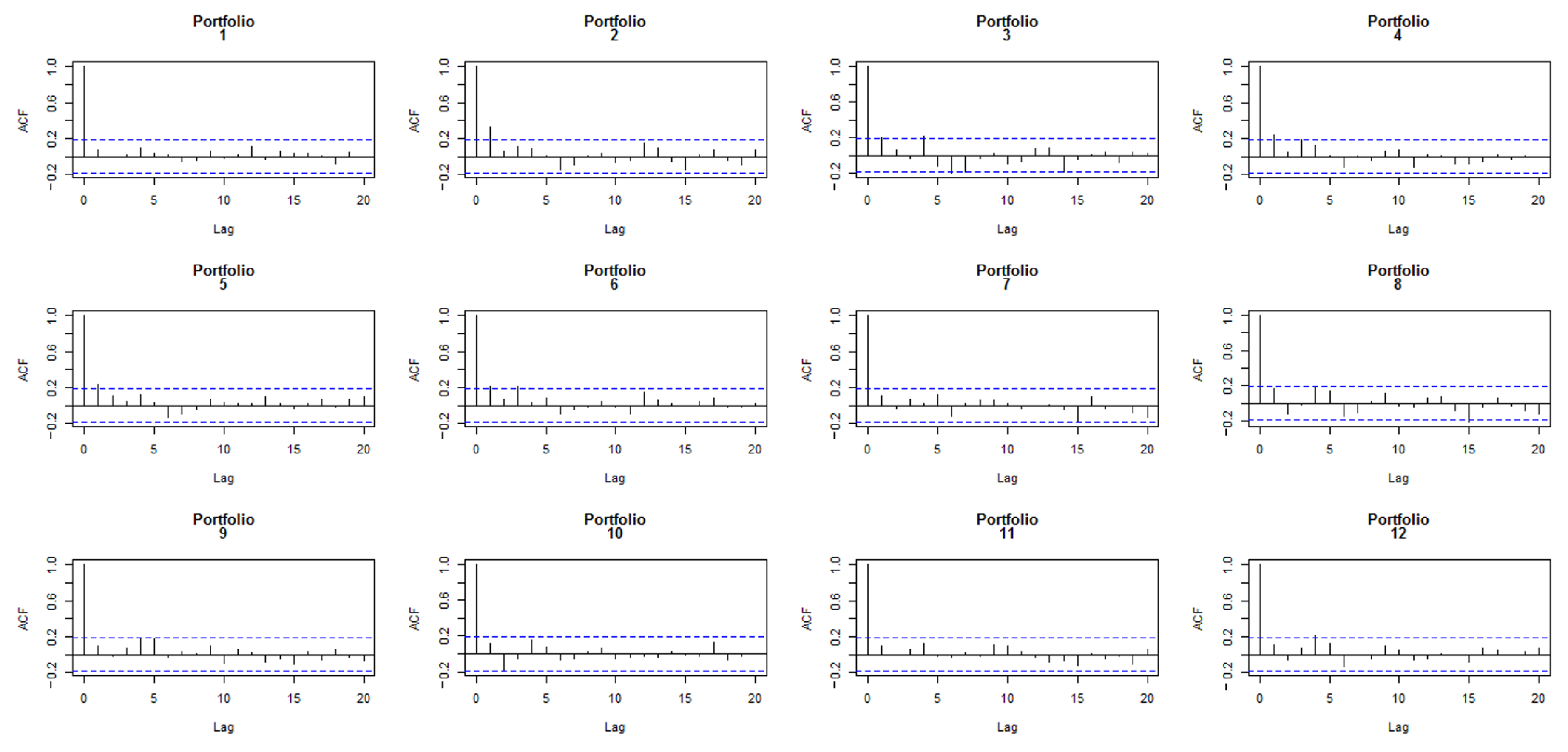
In order to confirm if the OLS hypotheses are fulfilled (normality, homoscedasticity, and independence), we performed several analyses similar to those in (Soumaré et al. 2013). A Shapiro–Wilk test was run on each set of residuals, suggesting that, in general, the residuals of the TS regression are normally distributed, except for portfolios 1-1-1 (p-value = $0.007$), 1-2-1 (p-value = $0.037$), and 1-2-2 (p-value = $0.024$). Additionally, charts of residuals vs. fitted values show that the homoscedasticity assumption is violated for portfolios 7 to 12 (high CV), see Figure 2. The Durbin–Watson test also suggests that errors may be autocorrelated for portfolios 2 to 6 (low CV). The autocorrelation charts plotted in Figure 3 indicate that residuals are especially correlated for lag equal to 1.

These three facts suggest that bootstrap might be useful to approximate the distribution of the GRS statistic. We obtained a bootstrap p-value of $5.4\%$, so we cannot reject that the $\alpha$ are jointly zero. We then observed the coefficients ($\alpha$ and $\beta$) generated for the 12 portfolios and noticed that: (1) All the bootstrap $\alpha$ CIs include zero, except for the last two portfolios ($\alpha$s are not only jointly zero, but individually zero also) and (2) all the $\beta$ CIs do not include zero (in fact, $\beta$ is positive in all of them).

Next, we incorporated the statistical factors one-by-one (coefficient of variation, skewness, and kurtosis). We found that the market coefficient estimates continued to be positive and statistically significant. In general, $\alpha$ were not statistically significant in any of the models.

3.1.2. Model 2: Market and Coefficient of Variation

In

Table 5. Results for Time-Series estimation of Model 2 (Market and CV).

	Estimates			t-Statistic			Bootstrap CI (2.5%,97.5%)
Portfolio	Alpha	Market	CV	Alpha	Market	CV	Alpha	Market	CV	Adj. ${\mathit{R}}^2$
1-1-1	0.0008	0.441	0.332	0.447	9.776	4.322	-0.002,0.005	0.344,0.562	0.209,0.430	0.700
1-1-2	0.0021	0.523	0.297	1.537	14.263	4.765	0.001,0.007	0.441,0.607	0.178,0.407	0.814
1-1-3	0.0012	0.541	0.235	0.587	9.562	2.449	−0.002,0.007	0.393,0.689	0.054,0.405	0.639
1-2-1	0.0022	0.471	0.275	1.539	12.520	4.300	0.001,0.007	0.386,0.561	0.140,0.390	0.773
1-2-2	0.0008	0.559	0.222	0.527	13.401	3.139	−0.002,0.005	0.453,0.669	0.087,0.326	0.773
1-2-3	0.0013	0.443	0.247	0.753	9.791	3.218	−0.001,0.006	0.346,0.552	0.061,0.395	0.670
2-1-1	0.0036	0.484	1.238	2.139	10.709	16.133	0.004,0.011	0.387,0.574	1.097,1.374	0.892
2-1-2	0.0024	0.539	1.202	1.746	14.576	19.131	0.002,0.008	0.462,0.608	1.065,1.317	0.929
2-1-3	0.0031	0.404	1.400	1.419	6.850	13.948	0.002,0.011	0.286,0.551	1.197,1.570	0.835
2-2-1	0.0016	0.427	1.198	0.949	9.783	16.144	0.000,0.007	0.345,0.518	1.062,1.341	0.886
2-2-2	0.0006	0.345	1.364	0.232	4.963	11.550	−0.004,0.006	0.196,0.514	1.115,1.564	0.763
2-2-3	−0.0033	0.490	1.217	−1.463	8.056	11.780	−0.012,−0.002	0.334,0.666	1.007,1.409	0.818

Notes. GRS: 1.9437, p-value: 0.038, p-value Boot.: 0.1326.

we present the results of the time-series estimation using the Market and Coefficient of Variation as factors. The coefficient estimates for Market and CV were always positive and statistically significant. Moreover, the portfolios with high loading on the CV factor had higher CV coefficients (interestingly, market coefficients stabilized around $0.5$ with respect to the previous model). Adjusted $R^2$ ranged between $63.9\%$ and $92.9\%$ and increased with respect to the previous model (especially in portfolios with high CV loading). Finally, the GRS test rejected the null hypothesis at $5\%$ that all pricing errors were equal to zero.

After applying our bootstrap procedure, we found that $13.26\%$ of the bootstrap values were greater than the obtained GRS statistic, so we could not reject the hypothesis that all the $\alpha$ were jointly zero. Actually, the bootstrap methodology offers a higher p-value than the one of the traditional methodology. Indeed, when we tried to fit an F distribution to the sampled GRS statistic, we found that the MLEs of degrees of freedom were $12.8$ and $33.6$, whereas the degrees of freedom in the denominator were far less than those in Equation (1). We then observed the coefficients ($\alpha$ and $\beta$) generated for the 12 portfolios, and we noticed that: (1) Six of the $\alpha$ CIs included zero, and (2) none of the $\beta$’s CIs (both Market and CV) included zero, being $\beta$ positive in all of them.

3.1.3. Model 3: Market and Kurtosis

In

Table 6. Results for Time-Series estimation of Model 3 (Market and Kurt).

	Estimates			t-Statistic			Bootstrap CI (2.5%,97.5%)
Portfolio	Alpha	Market	Kurt	Alpha	Market	Kurt	Alpha	Market	Kurt	Adj. ${\mathit{R}}^2$
1-1-1	−0.0007	0.541	−0.168	−0.396	12.563	−0.923	−0.005,0.002	0.436,0.674	-0.563,0.211	0.650
1-1-2	0.0008	0.614	−0.131	0.545	17.275	−0.871	−0.002,0.005	0.537,0.696	−0.486,0.191	0.776
1-1-3	0.0003	0.623	−0.004	0.158	12.130	−0.018	−0.004,0.006	0.482,0.767	−0.505,0.487	0.619
1-2-1	0.0014	0.588	0.213	0.925	16.507	1.421	0.000,0.006	0.506,0.681	−0.152,0.564	0.738
1-2-2	0.0005	0.682	0.452	0.348	18.387	2.892	−0.002,0.005	0.595,0.780	0.033,0.857	0.770
1-2-3	0.0008	0.563	0.337	0.437	13.692	1.942	−0.002,0.005	0.478,0.667	−0.106,0.757	0.651
2-1-1	−0.0026	0.796	−1.232	−0.921	11.644	−4.279	−0.011,0.001	0.655,0.952	−2.078,−0.541	0.684
2-1-2	−0.0037	0.841	−1.210	−1.392	13.373	−4.567	−0.013,−0.002	0.700,1.001	−1.977,−0.571	0.736
2-1-3	−0.0037	0.779	−1.179	−1.048	9.344	−3.357	−0.015,0.000	0.620,0.983	−2.103,−0.372	0.579
2-2-1	−0.0038	0.783	−0.656	−1.304	11.192	−2.224	−0.014,−0.002	0.654,0.933	−1.506,0.028	0.625
2-2-2	−0.0045	0.832	0.075	−1.162	9.037	0.194	−0.017,−0.001	0.647,1.045	−0.951,0.936	0.467
2-2-3	−0.0079	0.923	0.057	−2.305	11.337	0.166	−0.023,−0.009	0.751,1.127	−0.998,0.956	0.583

Notes. GRS: 1.767, p-value: 0.065, p-value Boot.: 0.086.

we present the results of the time-series estimation using the Market and Kurtosis as factors. The coefficient estimates for Market were always positive and statistically significant. Moreover, the portfolios with high loading on the CV factor had higher coefficients. However, coefficient estimates for the kurtosis change sign between portfolios (negative for low kurtosis ones and positive in the rest) and are only significant regarding classical methodology at standard levels for 5 of them (portfolios with low CV and high Kurt and portfolios with high CV and low Kurt). Adjusted $R^2$ registers lower values than in Model 2, going from $46.7\%$ to $77.6\%$, with marginal gains, in general, with respect to Model 1. The GRS test does not reject the null hypothesis at $5\%$ significance level.

When we apply the bootstrap methodology, we cannot reject the null hypothesis that all $\alpha$s are jointly zero, since we obtain a p-value of $8.6\%$ (higher than the one of the traditional methodology). Again, the second degree of the fitted F distribution is much lower than the one suggested by formula 1 (now the MLEs degrees of freedom are 12.2 and 35.2). Analogously as before, (1) seven of the $\alpha$ CI include zero, (2) all the market $\beta$ CI do not include zero (in fact, $\beta$ is positive in all of them) and (3) eight out of twelve of the kurtosis $\beta$ CI include zero, corresponding, in general, to those with low CV loading and those with high CV and high Kurt loading. This last fact emphasizes the small contribution of this statistical factor in explaining the returns of the twelve portfolios.

3.1.4. Model 4: Market and Skewness

In

Table 7. Results for Time-Series estimation of Model 4 (Market and Skew).

	Estimates			t-Statistic			Bootstrap CI (2.5%,97.5%)
Portfolio	Alpha	Market	Skew	Alpha	Market	Skew	Alpha	Market	Skew	Adj. ${\mathit{R}}^2$
1-1-1	0.0002	0.543	0.292	0.116	13.924	2.229	−0.003,0.004	0.461,0.645	0.070,0.602	0.663
1-1-2	0.0022	0.600	0.516	1.661	20.448	5.228	0.002,0.007	0.546,0.657	0.362,0.690	0.820
1-1-3	0.0021	0.586	0.704	1.052	13.703	4.893	0.000,0.008	0.490,0.676	0.439,1.010	0.689
1-2-1	0.0019	0.551	0.309	1.276	17.242	2.877	0.001,0.007	0.467,0.626	0.114,0.533	0.753
1-2-2	0.0011	0.612	0.478	0.760	18.687	4.335	−0.001,0.005	0.513,0.700	0.269,0.693	0.789
1-2-3	0.0023	0.489	0.784	1.561	15.590	7.430	0.002,0.007	0.418,0.559	0.578,0.996	0.762
2-1-1	−0.0004	0.904	0.289	−0.126	13.357	1.268	−0.007,0.005	0.746,1.065	−0.178,0.778	0.635
2-1-2	−0.0006	0.928	0.637	−0.216	15.306	3.121	−0.006,0.005	0.786,1.079	0.231,1.066	0.710
2-1-3	0.0011	0.827	1.329	0.323	11.617	5.549	−0.004,0.008	0.665,1.003	0.847,1.878	0.639
2-2-1	−0.0026	0.839	0.177	−0.852	12.762	0.801	−0.011,0.001	0.677,1.013	−0.344,0.723	0.610
2-2-2	−0.0023	0.775	0.943	−0.617	9.635	3.484	−0.012,0.003	0.594,0.964	0.322,1.651	0.521
2-2-3	−0.0040	0.832	1.638	−1.471	14.217	8.322	−0.013,−0.002	0.684,0.978	1.244,2.090	0.747

Notes. GRS: 1.8035, p-value: 0.051, p-value Boot.: 0.078.

we present the results of the time-series estimation using the Market and Skewness as factors. Using the classical methodology, the coefficient estimates for Market are always positive and statistically significant. The portfolios with high loading on the CV factor have the highest Market coefficients. Coefficient estimates for skewness are always positive (the higher the loading, the higher the coefficient) and are, in general, significant at standard levels (10 out of 12 portfolios). Adjusted $R^2$ levels (between $52.1\%$ and $82.0\%$) are better than those in Model 3, but worse than those in Model 2. Finally, the GRS test does not reject the null hypothesis at $5\%$.

On the other hand, $7.8\%$ of the bootstrapped values of the sample are higher than the GRS statistic. We then observe the coefficients ($\alpha$ and $\beta$) generated for the 12 portfolios and we notice that: (1) seven out of twelve of the $\alpha$ CI include zero, (2) all the market $\beta$ CI do not include zero (in fact, $\beta$ is positive in all of them) and (3) two of the skewness’ $\beta$ CI include zero.

3.1.5. Model 5: Market, Coefficient of Variation, and Skewness

In

Table A1. Results for Time-Series estimation of Model 5 (Market, CV and Skew).

	Estimates				t-Statistic				Bootstrap CI (2.5%,97.5%)
Portfolio	Alpha	Market	CV	Skew	Alpha	Market	CV	Skew	Alpha	Market	CV	Skew	Adj. ${\mathit{R}}^2$
1-1-1	0.001	0.441	0.306	0.175	0.639	9.815	3.889	1.381	−0.001,0.005	0.348,0.563	0.171,0.417	−0.063,0.485	0.702
1-1-2	0.003	0.522	0.234	0.427	2.282	15.469	3.962	4.476	0.003,0.009	0.455,0.593	0.115,0.351	0.257,0.608	0.842
1-1-3	0.002	0.540	0.140	0.651	1.252	10.347	1.528	4.420	0.001,0.009	0.425,0.666	−0.043,0.304	0.349,0.991	0.692
1-2-1	0.003	0.470	0.243	0.216	1.838	12.706	3.749	2.070	0.002,0.008	0.387,0.554	0.102,0.370	0.022,0.428	0.779
1-2-2	0.002	0.558	0.161	0.416	1.080	14.183	2.341	3.743	0.000,0.006	0.460,0.654	0.020,0.277	0.187,0.643	0.797
1-2-3	0.003	0.442	0.140	0.730	1.853	11.680	2.113	6.832	0.002,0.008	0.365,0.526	−0.015,0.255	0.522,0.959	0.769
2-1-1	0.003	0.484	1.267	−0.196	1.913	10.782	16.143	−1.551	0.003,0.010	0.387,0.575	1.125,1.403	−0.442,0.055	0.894
2-1-2	0.003	0.539	1.175	0.187	2.002	14.727	18.352	1.813	0.003,0.008	0.465,0.607	1.022,1.303	−0.022,0.402	0.930
2-1-3	0.005	0.404	1.276	0.840	2.412	7.795	14.082	5.749	0.005,0.013	0.308,0.514	1.094,1.445	0.528,1.176	0.873
2-2-1	0.001	0.427	1.242	−0.298	0.613	10.021	16.643	−2.476	−0.001,0.005	0.339,0.523	1.083,1.394	−0.479,−0.065	0.891
2-2-2	0.001	0.344	1.299	0.446	0.561	5.058	10.897	2.320	−0.002,0.008	0.196,0.498	1.067,1.487	0.141,0.844	0.772
2-2-3	−0.001	0.489	1.034	1.242	−0.598	11.200	13.550	10.084	−0.005,0.001	0.391,0.595	0.900,1.159	1.009,1.510	0.906

Notes. GRS: 1.7759, p-value: 0.063, p-value Boot.: 0.097.

we present the results of the time-series estimation using the Market, Coefficient of Variation, and Skewness as factors. According to the classical methodology, we find that the coefficient estimates for Market and CV are always positive and statistically significant (except for portfolio 1-1-3, where the t-statistic for ${\beta }_{CV}$ is 1.53). As in Model 2, the portfolios with high loading on the CV factor have higher CV coefficients and Market coefficients have stabilized around $0.5$. Coefficient estimates for Skewness are positive except for portfolios 2-1-1 and 2-2-1 (the higher the loading, the higher the coefficient) and are, in general, significant at standard levels (9 out of 12 portfolios). Adjusted $R^2$ ranges between $69.2\%$ and $93.0\%$ and reaches the highest values among the considered models. The GRS test does not reject the null hypothesis at $5\%$ significance levels.

When using the bootstrap methodology, we find that $9.70\%$ of the values of the sample are higher than the GRS statistic, so we cannot reject the hypothesis that all the $\alpha$ are jointly zero. We then observe the coefficients ($\alpha$ and $\beta$) generated for the 12 portfolios we notice that: (1) four of the $\alpha$ CIs include zero (mainly those with high CV and high Kurt), (2) none of the market $\beta$ CIs include zero (in fact, $\beta$ is positive in all of them), (3) two of the Coefficient of Variation $\beta$ CIs include zero (portfolios 1-1-3 and 1-2-3) and (4) only three of the skewness $\beta$ CIs include zero.

3.2. Cross-Sectional Regression

The only model that we consider in the present section is Model 5. Its GRS statistic (see Table A1 in Appendix A) suggests that we cannot reject that all $\alpha$s are jointly zero, and further, it registers the highest explained variability. Additionally, CV and Skew are statistically significant in most of the portfolios.

We use the $\beta$s estimated in Table A1 to examine if the factors are priced on the cross-section of returns. We must take into account that despite the fact that we are working with portfolios, risk premia will be estimated from the estimated coefficients, which can lead to an important bias, especially if the model is not well-specified.

As seen in

Table 8. Results for Cross-Sectional estimation of Model 5.

		t-Statistic
	Estimate	FM	CS	Bootstrap Basic 95% CI
Market	0.0102	2.0582	1.4853	0.0039, 0.0245
CV	−0.0015	−0.5816	−0.4020	−0.0070, 0.0039
Skew	−0.0026	−1.8070	−1.2878	−0.0060, −0.0006

, the highest risk premium is the Market one, which is $0.0102$, while the CV premium is estimated as $-0.0015$ and Skew premium is $-0.0026$. As a consequence, returns depend positively on the Market, and negatively on the CV and skewness factors. The reported t-statistics, which in the case of the CS ones include the Shanken correction (Shanken 1992), suggest that none of the factors are significant at conventional significance levels. However, bootstrap intervals indicate that Market and Skew $\lambda$s are significantly different from zero (at 5% level) contributing significantly to the model. The non significance of CV may be related to some multicollinearity problem. Note that the correlation between the market and the CV is around $0.6$ (see Table 2). However, we cannot reach the same conclusion for the CV factor, we still consider the current model (Model 5) superior to the other ones due to the superior explanatory power of its associated time-series regression models.

3.3. Comparison between Classical Methodologies and Bootstrap Methods

Given the existence of non-normality, heteroscedasticity and autocorrelation in the residuals of the regressions and, additionally, multicollinearity (high correlation among the different factors used in the analysis), we suspect that the estimates of $\alpha$, ${\beta }_i$ and GRS might not be very precise.

In

Table 9. Results Classical Methodologies and Bootstrap Methods.

		Number of Portfolios Where:				GRS
Model	Factors	${\mathit{\beta }}_{\mathit{m}}=0$	${\mathit{\beta }}_{\mathbf{cv}}=0$	${\mathit{\beta }}_{\mathit{k}}=0$	${\mathit{\beta }}_{\mathit{s}}=0$	p-Value	Adj. ${\mathit{R}}^2$
Model 1	M	0	-	-	-	0.038	0.776–0.472
Model 1b	M	0	-	-	-	0.054
Model 2	M, CV	0	0	-	-	0.038	0.929-0.639
Model 2b	M, CV	0	0	-	-	0.133
Model 3	M, K	0	-	7	-	0.065	0.776–0.467
Model 3b	M, K	0	-	8	-	0.086
Model 4	M, S	0	-	-	2	0.051	0.820–0.521
Model 4b	M, S	0	-	-	2	0.078
Model 5	M, CV, S	0	1	-	3	0.063	0.930–0.692
Model 5b	M, CV, S	0	2	-	3	0.097

, we compare the number of portfolios where ${\beta }_i=0$ for both methodologies: in the models without a sub-index we calculate different measures according to the classical methodologies, while in the models with a sub-index b, we calculate the same measures with the bootstrap. Indeed, when we observe the results presented in this table, we notice the p-values of the GRS Tests for bootstrap methodology are always higher than the ones obtained from the classical methodologies, showing that the former are more conservative (we fail to reject the null hypothesis that the $\alpha$ are jointly 0 more often). We also observe that the number of portfolios where ${\beta }_i=0$ varies depending on the methodology used.

4. Conclusions

We have defined three factors based on several statistical moments of stock prices. That is, the factors do not rely on external data, and thus can be used at any market. Based on them and in order to evaluate their relevancy, we have built 12 portfolios, and conducted a time-series and cross-section regression analysis.

In order to overcome the limitations of the classical tests commonly used in the factor-model literature, due to the strong assumptions about the data, we have proposed a block bootstrap inferential procedure. This procedure accounts for both potential cross-sectional and time-series correlation among returns and factors, while it allows to run all usual tests in factor models (GRS test on the intercepts of TS regression, test on the TS regression coefficients, and test on the CS regression coefficients).

The introduced technique has been used with data from several European stock markets which does not fulfill the requirements of the classical inferential techniques and has proven to be more conservative in terms of failing to reject the null hypothesis of the GRS test more often. After testing several models on data spanning from January 2008 to Febuary 2018, we propose one with three factors: market, skewness, and CV. The results are important for investors: they can improve the performance of their portfolios by considering long positions in stocks with low CV (in general, low variance and high prices) and low skewness and short positions in stocks with high CV and high skewness. This model has some drawbacks (specifically, the non-significance of the CV risk premium), which we think may be due to multicollinearity, but is an important explanatory power. In general, the model performance seems reasonably good in such a turbulent economic period in the Euro zone. The effect of including traditional factors in the model (size, profitability, cheapness, momentum, …) and the analysis of different time-periods is left for further research.

References

- Carhart, Mark M. 1997. On Persistence in Mutual Fund Performance. The Journal of Finance 52: 57–82. [Google Scholar] [CrossRef]
- Chang, Bo Young, Peter Christoffersen, and Kris Jacobs. 2013. Market skewness risk and the cross section of stock returns. Journal of Financial Economics 107: 46–68. [Google Scholar] [CrossRef]
- Conrad, Jennifer, Robert F. Dittmar, and Eric Ghysels. 2013. Ex Ante Skewness and Expected Stock Returns. The Journal of Finance 68: 85–124. [Google Scholar] [CrossRef] [Green Version]
- Efron, Bradley. 1972. Bootstrap Methods: Another Look at the Jackknife. The Annals of Statistics 7: 1–26. [Google Scholar] [CrossRef]
- Elyasiani, Elyas, Luca Gambarelli, and Silvia Muzzioli. 2020. Moment risk premia and the cross-section of stock returns in the European stock market. Journal of Banking & Finance 111: 105732. [Google Scholar]
- Fama, Eugene F., and Kenneth R. French. 1992. The cross-section of expected returns. The Journal of Finance 47: 427–65. [Google Scholar] [CrossRef]
- Fama, Eugene F., and Kenneth R. French. 1993. Common risk factors in the returns on stocks and bonds. Journal of Financial Economics 33: 3–56. [Google Scholar] [CrossRef]
- Fama, Eugene F., and Kenneth R. French. 2010. Luck versus skill in the cross section of mutual fund returns. The Journal of Finance 75: 1915–47. [Google Scholar] [CrossRef]
- Fama, Eugene F., and James D. MacBeth. 1973. Risk, Return and Equilibrium: Empirical Tests. Journal of Political Economy 81: 607–36. [Google Scholar] [CrossRef]
- Feng, Guanhao, Stefano Giglio, and Dacheng Xiu. 2020. Taming the Factor Zoo: A Test of New Factors. The Journal of Finance 75: 1327–70. [Google Scholar] [CrossRef]
- Gibbons, Michael R., Stephen A. Ross, and Jay Shanken. 1989. A test of the efficiency of a given portfolio. Econometrica 57: 1121–52. [Google Scholar] [CrossRef] [Green Version]
- Grané, Aurea, and Helena Veiga. 2008. Accurate minimum capital risk requirements: A comparison of several approaches. Journal of Banking and Finance 32: 2482–92. [Google Scholar] [CrossRef]
- Harvey, Campbell, and Akhtar Siddique. 2000. Conditional skewness in asset pricing tests. The Journal of Finance 55: 1263–95. [Google Scholar] [CrossRef]
- Jensen, Michael C. 1968. The performance of mutual funds in the period 1945–1964. The Journal of Finance 23: 389–416. [Google Scholar] [CrossRef]
- Kosowski, Robert, Allan Timmermann, Russ Wermers, and Hal White. 2006. Can mutual fund “stars” really pick stocks? New evidence from a bootstrap analysis. The Journal of Finance 61: 2551–95. [Google Scholar] [CrossRef]
- Kristjanpoller, Werner, and Carolina Liberona. 2010. Comparación de modelos de predicción de retornos accionarios en el Mercado Accionario Chileno: CAPM, Fama y French y Reward Beta. EconoQuantum 7: 121–40. [Google Scholar] [CrossRef]
- Kumar, Alok. 2009. Who gambles in the stock market? The Journal of Finance 64: 1889–933. [Google Scholar] [CrossRef]
- Lintner, John. 1965. The valuation of risk assets and the selection of risky investments in stock portfolios and capital budgets. Review of Economics and Statistics 47: 13–37. [Google Scholar] [CrossRef]
- Markowitz, Harry. 1952. Portfolio selection. The Journal of Finance 7: 77–91. [Google Scholar]
- Miller, Merton H., and Myron Scholes. 1972. Rates of return in relation to risk: A reexamination of some recent findings. In Studies in the Theory of Capital Markets. Edited by Michael C. Jensen. New York: Praeger, pp. 47–78. [Google Scholar]
- Morelli, David. 2010. European capital market integration: An empirical study based on a European asset pricing model. Journal of International Financial Markets, Institutions and Money 20: 363–75. [Google Scholar] [CrossRef]
- Mossin, Jan. 1966. Equilibrium in a Capital Asset Market. Econometrica 34: 758–83. [Google Scholar] [CrossRef]
- Ramos, Sofia, Abderrahim Taamouti, Helena Veiga, and Chih-Wei Wang. 2017. Do investors price industry risk? Evidence from the cross-section of the oil industry. Journal of Energy Markets 10: 79–108. [Google Scholar] [CrossRef] [Green Version]
- Shanken, Jay. 1992. On the estimation of beta-pricing models. The Review of Financial Studies 5: 1–33. [Google Scholar] [CrossRef]
- Sharpe, William F. 1964. Capital asset prices: A theory of market equilibrium under conditions of risk. The Journal of Finance 19: 425–42. [Google Scholar]
- Sørensen, Lars Qvigstad. 2009. Testing Mutual Fund Performance at the Oslo Stock Exchange. Available online: https://ssrn.com/abstract=1488745 (accessed on 19 October 2018).
- Soumaré, Issouf, Edo Jossi Aménounvé, Ousmane Diop, Dramane Méité, and Yao Djifa N’Sougan. 2013. Applying the CAPM and the Fama-French models to the BRVM stock maket. Applied Financial Economics 23: 275–85. [Google Scholar] [CrossRef]
- Viale, Ariel M., James W. Kolari, and Donald R. Fraser. 2009. Common risk factors in bank stocks. Journal of Banking and Finance 33: 464–72. [Google Scholar] [CrossRef] [Green Version]
Figure 1.
Portfolios’ cumulative returns.
Figure 2.
Residuals vs. fitted values in TS regression for CAPM.
Figure 3.
Autocorrelation charts for errors in TS regression for CAPM.