Evaluating the Performance of Islamic Banks Using a Modified Monti-Klein Model

Abstract

The development of Islamic banking continues to increase in many Muslim (majority) countries. Substituting interest with profit shares in the assets of a given Islamic bank as one of the bases of operation has many interesting implications, one of which is the need for more involved risk and return measures. In this paper, we take a balance sheet analysis-based approach to formulating profit in order to assess the performance of an Islamic bank. Then the implementation of this approach is demonstrated using data provided by Indonesia’s financial services authority, known as the OJK. We develop formulae for the calculation of profit share between funding and financing funds as well as the appropriate rates of return. The resulting figures are then used to construct statistical models for short-term forecasting of the volumes of funding fund from the depositors and financing fund for business people who need funds for their investment projects. The approach we develop is innovative for Islamic banks and would be a welcome addition to their performance assessment toolkit. One of the results of our model indicates an increasing pattern on the equivalent rates of returns for funding and financing funds every year, which is caused by the fact that the reported income from the financing fund seems to have been accumulated from the beginning until the end of year in the Islamic bank.

1. Introduction

1.1. Overview

The concept of an Islamic bank compels financial managers to adjust their strategies as their operations can no longer be based on borrowing and lending at a mark-up. More specifically, Islamic banks must seek out prospective projects and participate financially, establishing their stake and their right to a share of returns on said projects. One of the main implications of this is that a higher level of disclosure is expected as returns to investors are now a share of the fruits of a project instead of simply a number. While this also leads to a tighter relationship between the real and financial sides to the economy—as discussed in Siddiqi (2006) and Van Greuning and Iqbal (2009)—it naturally requires a more involved procedure for calculating the return (usually called nisbah) and risk of a project. Our intention is to delve into this aspect of Islamic banking, developing a return and risk measure for Islamic banks based on the Monti-Klein model of profit calculation as we shall elaborate. Aside from standard performance evaluation, we demonstrate that these measures can be used to facilitate the construction of statistical models which can help assess the prospects of a given Islamic bank.

1.2. Literature Review

Hassan and Aliyu (2018) provide a survey of studies comparing the profitability and returns of Islamic banks with conventional banks, demonstrating that these studies generally use regression and vector autoregression (VAR) models. One study of note is that of Zainol and Kassim (2010), who used the VAR framework to analyse market dynamics between conventional and Islamic banks in Malaysia. They found among other things that there is a negative relationship between the total deposit of Islamic banks and the interest rate of conventional banks. Doumpos et al. (2017) stated that there is no significant difference globally of the overall financial strength between Islamic and conventional banks. However, regionally, conventional banks outperform the Islamic banks in Asia and the Gulf Cooperation Council, but Islamic banks perform better in the Middle East, North Africa and Senegal region. Sumarti et al. (2017) shows that Islamic Banking growth in Indonesia has not given significant impact to Indonesia’s economic growth, even though the development of Islamic banks has been going for more than 20 years.

As for the suggestion in calculation of risk, some of the more rigorous approaches follow Van Greuning and Iqbal (2008) in explicitly modeling risk based on balance sheet assets and liabilities. Examples include Fadhlurrahman et al. (2016) and Sumarti et al (2018), who use deterministic systems of equations to model the dynamics of balance sheet items to predict given the banks’ deposit and loan evolution. Bidabad and Allahyarifard (2019) as well as Rahman (2019), use this approach to model optimal asset mixes for Islamic banks. Our review of the literature therefore indicates that while time series analysis and dynamics modeling have been employed, our use of the Monti-Klein model is relatively novel and should provide both contributions and new directions for the development of Islamic banking’s performance evaluation methods.

1.3. Outline

We will dedicate Section 2 to detailing our methodology in conducting this research and Section 3 to describing the data we use to implement the constructed models. Section 4 contains our results on evaluation of balance sheets of banks and subsequent analysis. Section 5 provides a summary of and our conclusions for this study including possible future directions for this strand of research.

2. Methodology

2.1. Overview

In a financial report, the information presented in the financial statements should be understood, relevant, reliable and comparable. According to the Statement of Financial Accounting Standards (PSAK), the financial statement is written as a form of the balance sheet.

Table 1. The balance sheet of a Sharia bank.

Financing (Assets)	Funding (Liabilities)
Murabahah (Mur), Istisna (Ist) Qard (Qrd), Ijarah (Ijr)	Wadiah Savings (WS), Wadiah Accounts (WA)
Mudarabah (Mud), Musharakah (Mus)	Mudarabah Savings (MS), Mudarabah Accounts (MA), Mudarabah Certificate of Deposit (MD)

shows the balance sheet of Islamic or Sharia bank, where the liabilities part or the source of fund is called Funding, and the assets part is called Financing. A formulation model on transforming the source of fund to become the application of fund theoretically in the balance sheet is rebuilt so we can calculate the equivalent rate of return for each source of fund. Using these calculated rates, the profit of a bank is estimated using Monti-Klein method, where some variables are modified in accordance with the balance sheet of Sharia banking. For the implementation of the model, in order to describe the situation and predict the near future, the statistical descriptive analysis is used to build time series models based on data of Sharia banks in Indonesia.

The statistical descriptive analysis used is in the form of time series methods. Time series methods, utilizing a series of data listed in time order, are used to illustrate the relationship between the current value of an observed variable and its values at previous time steps. Using the regression method, the profit or loss of a bank is estimated based on basic components of the balance sheet. We construct autoregression formulae based on the observation of the number of data lags and errors of regressions that are modeled, so we use Autoregressive Integrated Moving Average (ARIMA). It will be seen that we also need to implement seasonal factors in the time series in order to capture seasonal patterns in the data. The collected data is processed using statistical software, including R, which is one of the data analysis and simulation softwares that can provide visualization in accordance with the expected data processing.

2.2. The Modified Monti-Klein

The original Monti-Klein model as described by Freixas and Rochet (2008) is a constrained optimisation problem in which a monopolistic bank maximises its end of period net value by selecting the appropriate level of equity to raise as well as the rates it offers to depositors and prospective debtors. The main modification we make concerns how to calculate the bank’s rates which are different from conventional interest rates of deposits and loans. First, we take a look at the Islamic bank’s balance sheet. Originally, its exact composition varies depending on a particular bank’s business and market orientation. The funding structure of a bank directly affects its cost of operation and therefore determines a bank’s potential profit and level of risk. Harahap and Yusuf (2010) adds a third source of financing, a pool of funds for unrestricted investment, as it has features to distinguish it from conventional debt-based and equity-based financing. Specifically, it is a pool of funds raised through a Mudarabah Mutlaqah arrangement which basically makes it a dedicated investment account to be used at the bank’s discretion. The accounting equation is therefore now expressed as:

Asset = Liability + Unrestricted Investment + Equity

Next, the model of an Islamic bank balance sheet is constructed based on Muljono (2015) and Sumarti (2019), which is shown in Table 1. Let D be the size of the Islamic bank’s total pool of funds, which is called Funding. As per regulations, a part of it is deposited into a reserve fund R while the rest L is used to finance projects such that:

D(t) = L(t) + R(t)

(1)

We shall refer to L as the financing funds; the term “financing” is used instead of “investment”. Islamic banks also offer simple zero-interest loans referred to as Qard, which is only used as a supplement of investment funds without generating any profit. Regulations also require a portion of the reserve funds S must be held by the central bank and the remaining amount M as the net position in the interbank market due to some fund placement and liabilities in other banks. We therefore have:

R(t) = S(t) + M(t)

(2)

In accordance with the Monti-Klein model, funds (1) and (2) have associated returns and costs of financing. We introduce a cost function C(D,L) which represents a general cost of raising funds and putting them to use. This results in the following equation for a bank’s end of period net value, modified to reflect the circumstances of an Islamic bank:

π = total revenue − total cost

$$\pi (D,L)=r_{L}L(t)+rS(t)+rM(t)-r_{D}D(t)-C(D,L).$$

(3)

where $r$ reflects the rate of the interbank market, and equivalent rates of returns for funding $r_D$ and financing $r_L$ will be formulated in Equations (9) and (12).

As we have discussed above, Islamic banks can raise funds through various financial contracts. In practice, the main modes of fundraising are through Wadiah and Mudarabah contracts. These collectively come in five different categories: Wadiah savings ($D_1$), Wadiah accounts ($D_2$), Mudarabah savings ($D_3$), Mudarabah accounts ($D_4$) and Mudarabah certificate of deposit ($D_5$). Note that Wadiah are pure deposit contracts which cannot be utilized for financing without permission from the owner. There is no permission in $D_1$ and there exists one in $D_2$, but the return of financing in $D_2$ is usually in a form of uncertain bonuses, which is not discussed here. Therefore, we define the following:

$$D(t)=D_1(t)+D_2(t)+D_3(t)+D_4(t)+D_5(t).$$

(4)

In relation to the requirement that a portion of D must be held in reserve,

Table 2. Values of $\alpha$ for each type of funding.

Type of Funding	Weight (α)
Accounts	89%
Savings	90%
Certificate of Deposit (Mudarabah)	91%

demonstrates the portions of the constituents of D that are generally available for financing based on Sumarti (2019). For example, the weighted amount of Mudarabah savings that can be used as financing fund is 90% $D_3(t)$. We denote ${\alpha }_i$ to be the portion of a given $D_i$ that may be used for financing.

The financing fund L is allocated to the following contracts: Murabahah ($L_1$), Istisna ($L_2$), Qard ($L_3$), Ijarah ($L_4$), Mudarabah ($L_5$) and Musharakah ($L_6$) contracts. There is also a defined ε which accounts for any discrepancies between the total amount available for financing ${\displaystyle \sum _{i=1}^5{\alpha }_i{D}_i}(t)$ and the total value of the financing funds $\mathrm{L}\left(\mathrm{t}\right)$. The financing fund L can be written as follows

$$L(t)=L_1(t)+L_2(t)+L_3(t)+L_4(t)+L_5(t)+L_6(t)+\epsilon (t).$$

(5)

The weighted deposit ${\displaystyle \sum _{i=1}^5{\alpha }_i{D}_i}(t)$ is supposed to be entirely distributed into financing fund $L(t)={\displaystyle \sum _{j=1}^6{L}_j}(t)$. This can be true if ${\displaystyle \sum _{i=1}^5{\alpha }_i{\mathrm{D}}_i}(t)=L(t)$, which is not always happening. We define $D_j{}^L$ to be the real amount of funding being distributed to the financing $L_j,j=1,2,\dots ,6$, which can be written as follows:

$$D_j{}^L(t)=\frac{L_j(t)}{L(t)}{\displaystyle \sum _{i=1}^5{\alpha }_i{D}_i(t)}.$$

(6)

We consider two possibilities on the discrepancy between two funds, $L(t)$ and ${\displaystyle \sum _{i=1}^5{\alpha }_i{D}_i}(t)$.

$$\mathrm{Case} 1. {\displaystyle \sum _{i=1}^5{\alpha }_i{D}_i}(t)\ge L(t)$$

This means there is a remaining fund from the weighted deposit that is not applied to the financing fund. We assume this remaining fund is used in another project ε(t), so

$$\epsilon (t)={\displaystyle \sum _{i=1}^5{\alpha }_i{D}_i}(t)-L(t).$$

(7)

Consequently, we observe that the financing fund is all sourced from the weighted deposit.

$$D_j{}^L(t)={\displaystyle \sum _{i=1}^5{\alpha }_i{D}_i}(t)-\epsilon (t)=L_j(t).$$

$$\mathrm{Case} 2. {\displaystyle \sum _{i=1}^5{\alpha }_i{D}_i}(t)<L(t)\mathrm{or}\frac{{\displaystyle \sum _{i=1}^5{\alpha }_i{D}_i}(t)}{L(t)}<1$$

The weighted deposit is not enough to finance all financing fund $L(t)$ and consequently $\epsilon (t)=0$. We assume the weighted D is distributed evenly on all financing fund $L_j(t)$. Financing fund which is not sourced from the weighted deposit is obtained from the bank’s other source not considered in this research.

The equations being constructed above define a given Islamic bank’s financing and funding funds and their financial constraints in accordance with the original Monti-Klein model. To complete the setup, we formulate the equivalent rates of return for all of the bank’s associated financial contracts. As explained before, Islamic banks obtain their income by participating in profitable projects. It requires data of financing income from the monthly income statement and other comprehensive income reported in the balance sheet. Let $I_j(t)$ be income at time-t from j-th contract in financing fund. For example, $I_5(t)$ is the total income shared from the entrepreneurs in the Mudarabah contract at time-t. This shared income is distributed to all depositors in the funding funds in a certain proportion, which is defined as follows:

$$P_j{}^L(t)=\frac{D_j{}^L(t)}{L_j(t)}\times I_j(t).$$

(8)

where $P_j{}^L(t)$ is the profit share from financing fund $L_j(t)$, $j=1,2,\dots ,6.$ For case 1 above, $P_j{}^L(t)=I_j(t)$. The equivalent rate of return $r_L$ for the financing fund $L(t)$ is simply defined as follows,

$$r_L(t)=\frac{{\displaystyle \sum _{j=1}^6{P}_j{}^L(t)}}{L(t)}$$

(9)

Profit shared ${\displaystyle \sum _{j=1}^6{P}_j{}^L(t)}$ will be distributed to the depositors for each funding fund and to the bank itself based on the profit shared proportion (nisbah). The gross profit share for i-th funding contract is defined as follows, for $i=1,2,\dots ,5.$

$$P_i{}^D(t)=\frac{{\alpha }_i{D}_i(t)}{{\displaystyle \sum _{i=1}^5{\alpha }_i{D}_i}(t)}\times {\displaystyle \sum _{j=1}^6{P}_j{}^L(t)}.$$

(10)

The share proportion (nisbah) might be varied among Islamic banks. We used nisbah guidelines set by the Indonesian central bank, Bank Indonesia (BI), which is shown in

Table 3. Share proportion (nisbah) of funding fund.

Funding Contract	Nisbah Ni
Wadiah accounts (WA)	6%
Wadiah savings (WS)	9%
Mudarabah accounts (MA)	6%
Mudarabah savings (MS)	21%
Mudarabah deposit (MD)	45%

. Here we assume the bonus for Wadiah contract is available and constant. Note that theoretically, the bonus is fluctuated depending on each bank policy.

The net profit share for the depositors of i-th funding fund $P_i{}^N$ is defined as follows

$$P_i{}^N(t)=N_i\times P_i{}^D(t)$$

(11)

Here $N_i$ is the nisbah for i-th contract. Consequently, the net profit share for the bank is $(1-N_i)P_i{}^D(t)$. The equivalent rate $r_D$ is simply defined as the average of the rates of return of all deposits.

$$r_D(t)=\frac{1}{5}{\displaystyle \sum _{i=1}^5\left(\frac{P_i{}^N(t)}{D_i(t)}\right)}.$$

(12)

In Equation (12) above, the net profit is divided by the deposit, not the weighted deposit, because the rate should be calculated with respect to the real amount written in depositors’ account balance.

Now we calculate the bank’s profit or loss using Monti Klein model as in the Equation (3), which can be expressed as

$$\pi (D,L)=r_L{L}_D(t)+rS(t)+r{D}_{BL}(t)-r{L}_{BL}(t)-r_{D}D(t)-C(D,L).$$

(13)

where $L_D(t)={\displaystyle \sum _{j=1}^6{D}_j{}^L(t)}$ is total funding fund distributed to the financing fund. Rate r is the equivalent rate of return from the interbank market. We assume its value is the same as Central Bank’s monthly interest rate. The term is the total fund borrowed by the bank at the time t, and its value is collected from the balance sheet. The variable S(t) is the cash reserves, which in this case is securities owned by the bank at the time t. $L_{BL}(t)$ is total financing fund borrowed by other banks at time t. Management cost $C(D,L)$ is taken from the reported profit and loss statement and other comprehensive incomes in the monthly report.

2.3. Regression Model

Having constructed formulae for a given Islamic bank’s size of funding, financial assets, associated rates of return and profit, we use the resulting data to estimate ARIMA models for selected Islamic banks. The model finds a causal relationship between a variable of response (dependent) and a predictor variable (independent). The causal relationship is demonstrated by the correlation values describing the linear relationship between two random variables where the value is between −1 and 1. Detailed explanation on time series models can be found in Wei (2006); Ruppert (2010) and Cryer and Chan (2018). If the regression equation with one independent variable involves a p-order autoregressive error structure (AR), meaning p times differencing process, the equation will be the form of

$$Y_t={\alpha }_0+{\varphi }_1{Y}_{t-1}+\dots +{\varphi }_p{Y}_{t-p}+{\alpha }_1{X}_t+{\alpha }_2{X}_{t-1}+\dots +{\alpha }_p{X}_{t-p}+{\epsilon }_t$$

(14)

where ${\alpha }_0$ is a constant parameter, ${\varphi }_1,\dots ,{\varphi }_p$ are parameters respectively related to the response variable at time lags $t-1,\dots ,t-p$ and ${\alpha }_1,{\alpha }_2,\dots ,{\alpha }_p$ are parameters respectively related to the predictor variable at time lags $t,t-1,\dots ,t-p$. For example, ARIMA (1,1,0) has the equation with the form of

$$Y_t={\alpha }_0+{\varphi }_1{Y}_{t-1}+{\varphi }_2{Y}_{t-2}+{\alpha }_1{X}_t+{\alpha }_2{X}_{t-1}+{\alpha }_3{X}_{t-2}+{\epsilon }_t.$$

The data also strongly suggests that there are seasonal effects, which makes it more appropriate to use a more generalised form of the ARIMA model. This form combines seasonal factors in a multiplicative and is denoted as ARIMA $(p,d,q)\times {(P,D,Q)}_S$ where nonseasonal parameters $p,d,q$ are respectively the order of AR, differencing process and MA, and parameters $P,D,Q$ are respectively their related seasonal parameters; $S$ is the number of time lags until the pattern repeats itself. For example, a yearly pattern data with ARIMA $(1,0,0)\times {(1,0,0)}_{12}$ without a predictor variable has the equation with the form of

$$Y_t={\alpha }_0+{\varphi }_1{Y}_{t-1}+{\alpha }_1{Y}_{t-12}+{\alpha }_2{Y}_{t-13}+{\epsilon }_t.$$

(15)

In the implementation, the formulae and statistical models are used for forecasting. To this end, we use the first 43 months as training data and the remaining 5 months as validating data. Lastly, there is the issue of controlling for bank and/or asset size. The Indonesian central bank has established the Bank Umum Kelompok Usaha or Commercial Bank Group (BUKU) classification (to be elaborated upon in Section 3) for banks based on the size of their primary equity. More specifically, our sample comes from selecting a bank from each of the three (out of four) classification tiers. We then apply our tools of analysis to each in separation and compare the results. We consider ourselves justified in this approach as our main goal is to construct measures of performance that can better accommodate the idiosyncrasies of Islamic banks.

3. Data Implementation

3.1. Original Data

In this research, data being used is publically available data from some prominent Islamic banks in Indonesia which can be obtained from the website of Indonesia’s financial services authority at www.ojk.go.id. The data consists of the banks’ monthly income statements during the period April 2015–March 2019. Banks in Indonesia are subject to the BUKU (Bank Umum Kelompok Usaha or Commercial Bank Group) classification as outlined in Bank Indonesia regulation No. 14/26/PBI/2012: BUKU 1, the first tier consists of banks with primary equities of less than one trillion IDR; BUKU 2 consists of banks with primary equities between one trillion IDR (inclusive) and five trillion IDR (exclusive); BUKU 3 consists of banks with primary equities between five trillion IDR (inclusive) and thirty trillion IDR (exclusive); and BUKU 4 consists of banks with primary equities above thirty trillion IDR (inclusive). Note that there are no BUKU 4-tier Islamic banks so our samples represent the first three tiers denoted Bank A for BUKU 1, Bank B for BUKU 2 and Bank C for BUKU 3. For the presentation in tables later in this section, we use a sample of full year coverage of years 2016, 2017 and 2018.

Having examined the balance sheet of each bank, we provide an example of the balance sheet from Bank C for January 2016 whose primary equity was between 5 and 30 trillion IDR. Figures of other banks can be seen in Appendix A. Figure 1 shows real data of funding and financing funds, which are both increasing, as well its financing income, which generally seems to increase gradually throughout the year and drop sharply towards the end. We suspect that this is because there are banks in Indonesia which are required to report their incomes in a cumulative manner such that income from one month carries over until the end of the financial year. However, it is also possible that the banks generally deal in short-term financing such as operational financing so it makes sense for their business activities to grow throughout the year. As we were unable to ascertain which one of these is the case, we have not controlled for cumulative income. Later, the pattern will result also in a yearly pattern of the equivalent rates of returns.

It can be observed that Bank C primarily raises its funds through Mudarabah certificates of deposit (MD) and mainly invests its funds into Murabahah contract (Mur). Note that Bank C does not provide Istisna credit, which is basically a credit facility to preorder goods that need to be made or built first.

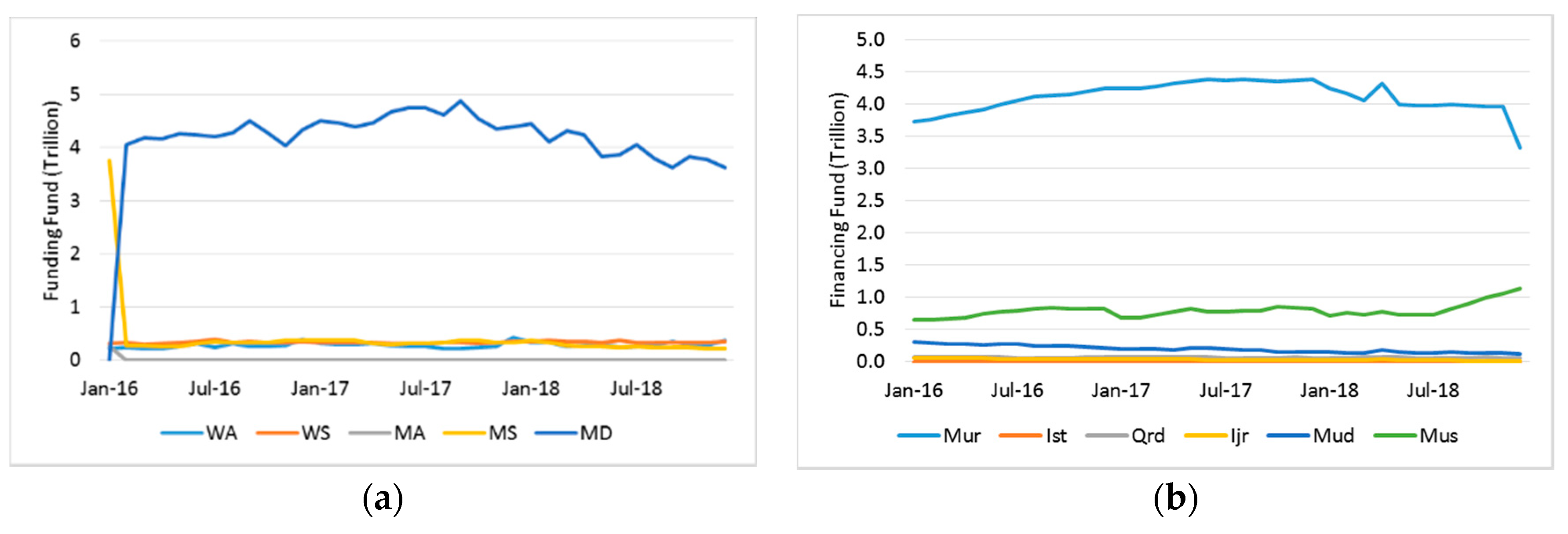
Composition of funding and financing funds for all banks are shown respectively in Figure 2 and Figure 3. In Figure 2, the amount of Mudarabah Deposit (MD) dominates significantly in A and B, which is about 80%. The amounts of other funds are much smaller, which are about 16% and lower. Furthermore, in Bank B, the amount of Mudarabah Account is zero starting from February 2006. In January 2006, there is no value for Mudarabah Deposit in Bank B, and it suddenly exists and dominates starting from February 2006. In Bank C, the composition of Mudarabah Deposit also dominates the balance sheet but the percentage is about 44.2% to 55% in a decreasing trend. There are two amounts, Mudarabah Saving and Wadiah Saving, which increase their percentages respectively from 25.2% to 28.8% and from 85% to 18.3%.

In Figure 3, Murabahah contract dominated the financing fund for Bank A and C, where the percentages are respectively from 71.1% to 81.6% and from 64.1% to 76.2%. In Bank B, the amount of Murabahah contract slightly dominates from 50.8% first but it decreases up to 36.3%. On the other hand, Musharakah contract increases from 39.9% to 61%.

3.2. Application of Constructed Formulae

We use figures from Bank C’s statements for January 2016, as summarised in

Table 4. Jan 2016 balance sheet of Bank C (IDR, million).

FINANCING		Income	FUNDING		Weighted Fund	Profit Share	Equivalent Rates
Mur	13,490,168.00	154,732.00	WA	1,029,204.00	915,991.56	11,122.13	0.000648
Ist	0.00	0.00	WS	1,705,314.00	1,534,782.60	18,635.61	0.000984
Qrd	574,756.00	0.00	MA	554,943.00	493,899.27	5997.01	0.000648
Ijr	233,185.00	7543.00	MS	5,804,091.00	5,223,681.90	63,426.88	0.002294
Mud	1,256,026.00	12,722.00	MD	11,041,464.00	10,047,732.24	122,001.37	0.004972
Mus	2,179,779.00	18,590.00
Total (1)	17,733,914.00
Other	482,173.57	27,596.00
Total (2)	18,216,087.57	221,183.00		20,135,016.00	18,216,087.57	221,183.00

, to give examples on adjustments to the funding and financing funds if their amounts differ. These adjustments should be done before the calculation of gross and net profit share. In January 2016, Bank C has IDR 20.135 trillion from funding funds. After the funding funds are multiplied by their weights using Table 2, the total becomes IDR 18.216 trillion. On the financing side, the total financing funds is IDR 17,734 trillion (in cell Total (1) on Table 4), which is less than IDR 18.216 trillion. This is case (1) on page 4. We assume there is another investment financed by the difference in Equation (7), so the total of the financing fund is now IDR 18.216 trillion (in cell Total (2)).

At the end of the month, the total profit resulting from financing activities is IDR 221.183 billion, as in Total (2) on the “Income” column. This total is shared and passed on to the funding funds’ side such that the amount is the same as the Total (2) on the “Profit Share” column. Note that Qard (interest-free loans) under the column of financing fund items do not generate profit as per the definition. Having calculated the nisbah part using Table 3, the equivalent rates of return for funding funds are about 0.0648–0.4972% per month or 0.1909% using Equation (12). On the other hand, the equivalent rate of return for financing is on average 1.214% using Equation (9). We conduct the same calculation for all the data of banks.

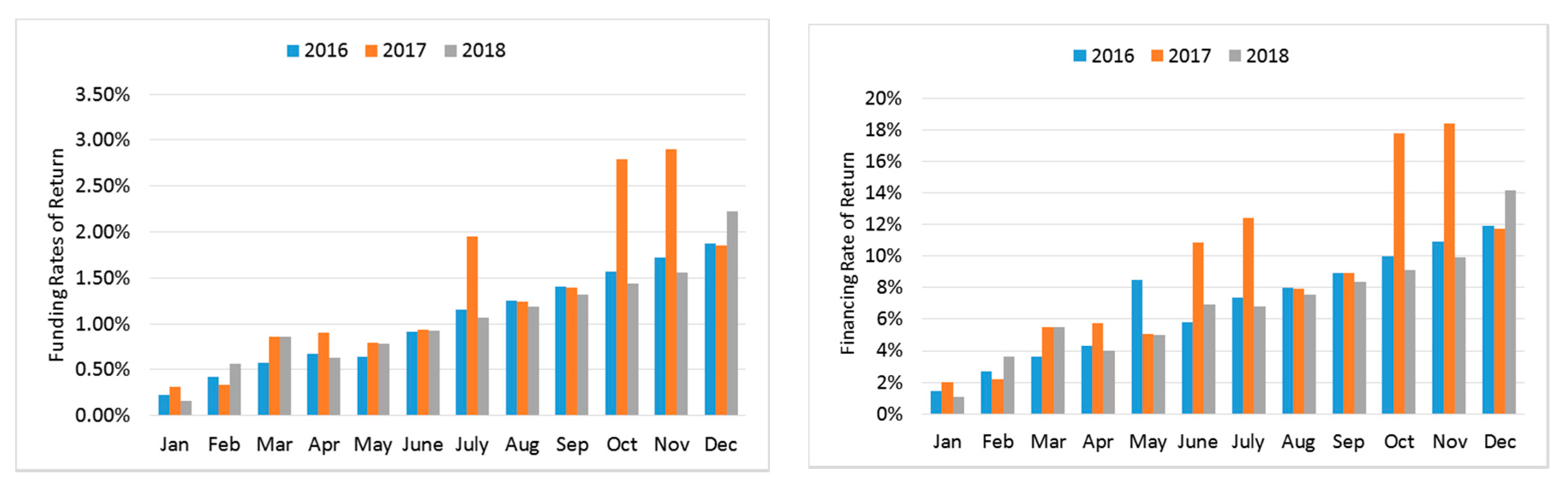
Figure 4 shows the monthly equivalent rates of return for financing (left) using Equation (12) and funding (right) using Equation (9) for Bank C. The financing rates are higher than the funding rates because the latter is already calculated using nisbah. It is observed that the monthly rates are increasing from the beginning to the end of the year. This pattern is consistent with the pattern of income in Figure 1 being lower. This pattern is consistent with the pattern of income as shown in the lower graph in Figure 1. As discussed before, we suspect that the steadily increasing pattern is due to the bank’s monthly income being recorded in a cumulative manner such that the calculated equivalent rate in December represents the bank’s annual return. The figure also shows that the higher rates are in year 2016, and then they decrease year by year. Graphs of the monthly rates of return for the other banks can be seen in Appendix B.

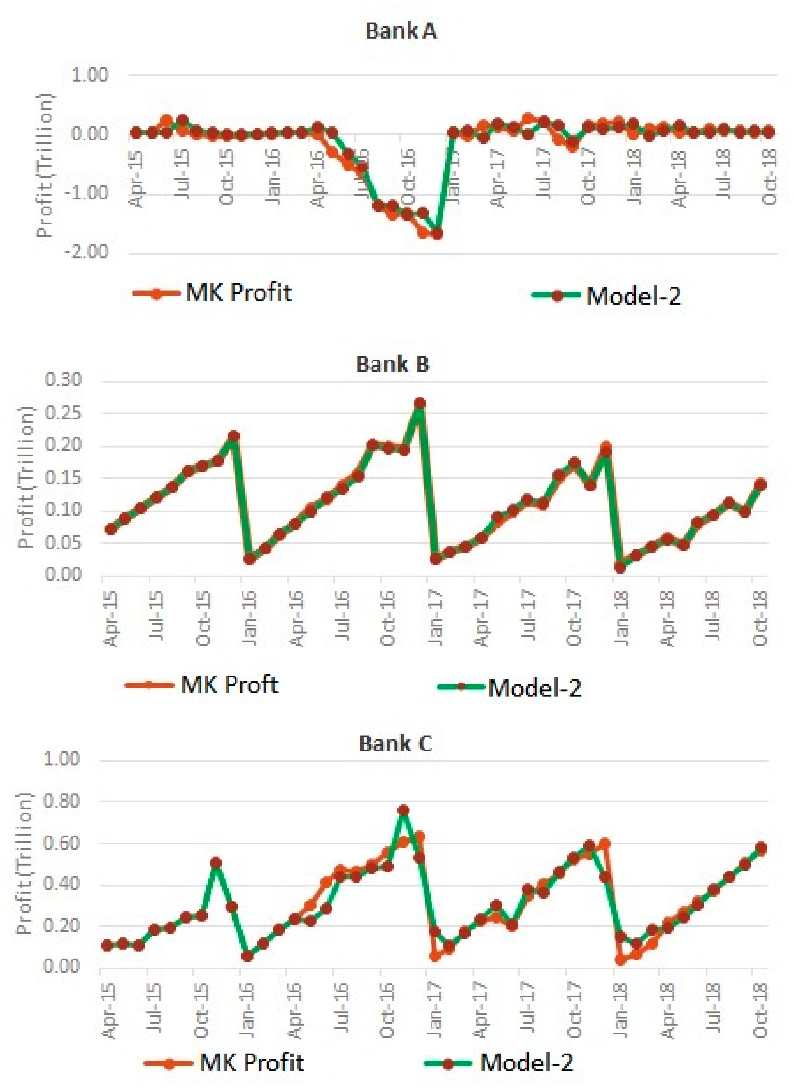
Now we calculate the bank’s profit based on Monti-Klein model. Note that the periodical bank’s report in the website also includes the profit. However, the formula of this reported profit is undisclosed and we find it differs across banks. Our recalculation of the bank’s profit using Monti-Klein model therefore provides a clearer relationship on how the basic components of the balance sheet are related. In Figure 5, the calculated profit on Bank A shows relatively deep losses during May–December 2016. A large inconsistency of a few data among other data hints at possible outliers. We can scan the existence of them and do a hypothetical test as to whether they are outliers or not. If outliers exist, it could improve the estimation process by the time series but sometimes it cannot do the same in the forecasting process. This will be discussed in the next section. The profit graphs of Bank B and Bank C are shown respectively in Figure 6 and Figure 7. They have seasonal structure which is later successfully be estimated using Regression model Note that this calculated Monti-Klein profit cannot be compared to the written profit in the bank’s monthly report because we only consider profit generated from the main components of the bank’s balance sheet. An example of written operational profit of all banks, which is very different from Figure 5 below, can be seen in the end of Appendix A.

4. Models for Estimation

Having examined Figure 5, Figure 6 and Figure 7, we develop the regression model of profit function with respect to funding fund, because the profits/losses being considered are the income of obtained funding fund from the third party or customers. Let $Y_t$ be the size of profit and $X_t$ be the size of funding fund of the bank. As mentioned above, there is a potential outlier in the data that can be accommodated into the model. For Banks B and C, the models should capture seasonal pattern. Using 43 data points for each bank’s profits/losses, we do preliminary data analysis such as stationary of data, correlation on the errors by inspecting Autocorrelation Function (ACF) and Partial Autocorrelation Function (PACF) plots and value estimation of parameters. In the process, there are potential models to be considered and finally we choose the best one. As the goodness-of-fit measures, we use Root Mean Square Error (RMSE), which means the smallest error compared to the observed data, and R-squared, indicating the percentage of variance in the dependent variable that the independent variables explain collectively. The best model has the smallest value of RMSE and R-squared among other potential models that are discussed here. Those values for each bank are shown in

Table 5. Goodness of fit.

Bank	Models-1		Models-2 (Outliers)		Forecast Models-1	Forecast Models-2
	RMSE	R-Squared	RMSE	R-Squared	RMSE	RMSE
A	307,356.9	0.62	124,412.5	0.94	65,067	210,860
B	20,092.3	0.89	2689.0	0.99	21,919	218,251
C	86,310.0	0.76	55,717.1	0.90	26,420	131,600

.

Data of Bank A need to be differenced once to make them stationary and then the best model is ARIMA (1,1,0). Bank B and Bank C data show the existence of a seasonal or seasonal structure with a 12-month period on the ACF and PACF structures so that the error is modeled with ARMA ${(1,0,0)\times (1,0,0)}_{12}$. Models for Banks A, B and C, called Models-1, are respectively:

$$\begin{gathered} Y_t=0.998Y_{t-1}+0.002Y_{t-2}+0.03X_t-0.023X_{t-1}-0.007X_{t-2}+132.5 \\ {Y}_t=0.648Y_{t-1}+0.917Y_{t-12}-0.549Y_{t-13}+0.03X_t-0.017X_{t-1}-0.023X_{t-12}+0.015X_{t-13}-2076 \\ {Y}_t=0.709Y_{t-1}+0.768Y_{t-12}-0.544Y_{t-13}-0.011X_t+0.007X_{t-1}-0.008X_{t-12}+0.005X_{t-13}+318300 \end{gathered}$$

The estimated profits generated from these models are shown in Figure 5, Figure 6 and Figure 7 respectively for Banks A, B and C. The values of RMSE and R-squared of Models-1 are shown in Table 5. RMSE value for Bank A is still large because the Monti-Klein data of Bank A has an extreme value with very large deviation, which is the lowest lost IDR 15.183 billion in October 2015. The R-squared value of Bank A’s model is the lowest among the values of other banks. The residual normality test is to see whether the plot of the residue follows a straight-line graph or not.

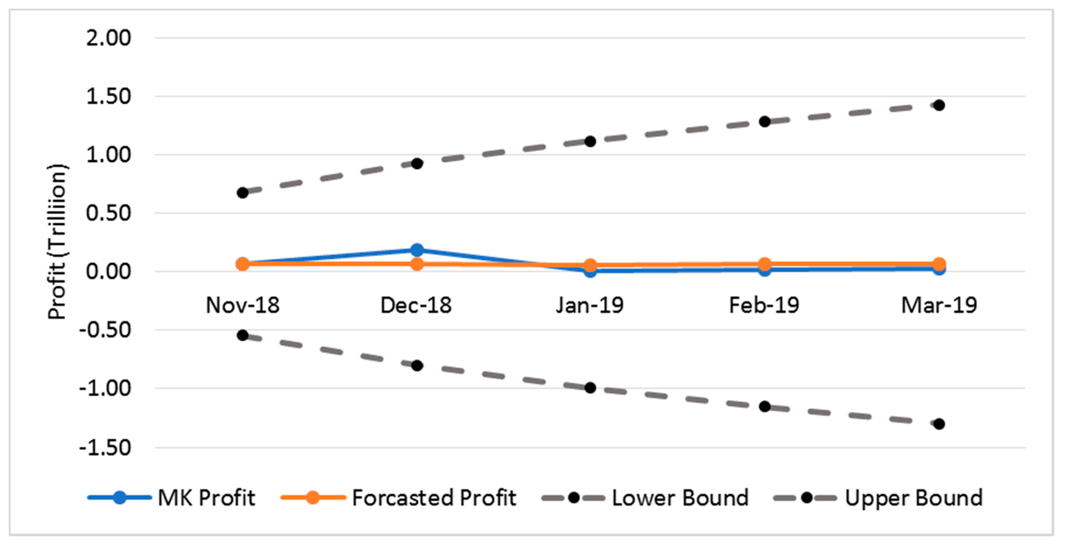
For the forecasting process, the model is equipped with 95% confident interval where the good forecasted data can be anywhere inside the interval. Figure 6 shows the forecasted profit is quite close to the MK profit of Bank A, except for data on December 2018. As previously stated above, very large deviation of data results in a very large width of obtained confidence interval, which is shown in Figure 8 and

Table 6. The forecasted profit of Bank A in IDR trillion.

Components	November 2018	December 2018	January 2019	February 2019
Forecast	65.878	64.012	60.165	63.786
Observation	65.262	186.007	9.290	16.798
Deviation	617	121.995	50.875	46.988
Bottom bound	543.659	−796.888	−993.766	−1152.926
Upper bound	675.416	924.914	1114.095	1280.498

. The largest deviation occurs in January 2019, which is 547%. The RMSE of the forecast profits can be found in Table 5.

Now we show revised models considering outliers identification to improve RMSE and R-squared values, so the estimated profits are much closer to the observed ones. However, in Table 5 forecasting values of Models-1 are better than that of Models-2, which are revised by the outlier identification. At the end, we will still choose Models-1 as the best forecasting models.

Based on Chang et al. (1987), there are two kinds of outlier; Additive Outliers (AO), which is an event only having an effect on a period of time, and Innovational Outlier (IO), which is an event having effects on subsequent events. We give an example of the model-2 for Bank A, and the other models-2 are in the Appendix C. There are three IO data, which have indices 22 (Jan-17), 17 (Aug-16) and 31 (Oct-17) respectively. New models considering outliers are in the form of

$$Y_t=0.0197Y_{t-1}+0.0391X_t+\frac{1}{1-0.0197Y_{t-1}}\left(1747203.4I_t{}^{(22)}-529929I_t{}^{(17)}+381237I_t{}^{(31)}\right)$$

$$I_t{}^{(k)}=\{\begin{array}{cc}1,& k\mathrm{is}\mathrm{outlier},\\ 0,& \mathrm{others}.\end{array}$$

The obtained values of R-squared are now closer to 1, which is also shown in Table 5. However, the forecast profit has higher RMSE, which is shown in Table 5. The values of forecast profits for all Banks are in Appendix C. Going forward, we consider Models-1 as the best model.

Figure 6 and Figure 9 show respectively the graphs of the MK profit and forecast profit of Bank B. The forecast points are almost coincided with the observed ones, except for data on December 2018. See

Table 7. Forecast profit of Bank B in IDR trillion.

Components	November 2018	December 2018	January 2019	February 2019
Forecast	120.088	176.369	16.580	33.245
Observation	119.179	128.613	19.289	40.900
Deviation	909	47.756	2.709	7.655
Bottom bound	80.708	129.445	−33.171	−17.646
Upper bound	159.468	223.293	66.331	84.137

for the detailed deviations. The largest deviation occurs in December 2018 but its value is 37.1%. For Bank C, the graphs of the MK profit and forecast profit are respectively in Figure 7 and Figure 10, and the related deviation is in

Table 8. Forecast profit of Bank C in IDR trillion.

Components	November 2018	December 2018	January 2019	February 2019
Forecast	557.564	595.328	158.111	173.571
Observation	612.659	652.843	34.839	148.716
Deviation	55.095	57.515	123.272	24.855
Bottom bound	388.399	387.942	−66.048	−58.567
Upper bound	726.728	802.714	382.271	405.709

. The largest deviation occurs in January 2019, which is 353%, but the forecast values are still inside the confidence interval. In general, Regression Models-1 perform satisfactorily.

5. Discussion of Results

5.1. The Developed Methodology

The methodology we have developed for the performance evaluation of Islamic banks is effective for two main reasons: firstly, it is more “asset-” or “business-centric” and hence more true to the essence of Islamic finance; secondly, it provides a more conceptually robust approach to calculating an Islamic bank’s net income. Regarding the first reason, our methodology forces the identification of an Islamic bank’s sources and uses of funding as well as their underlying contracts. This is significant because the various contracts have differing characteristics which can help in identifying the environment in which the bank is operating. An example of this is the classic “murabahah syndrome” in which Islamic banks will go against their stated preference for profit-sharing and instead prefer fixed-income contracts such as Murabahah. There could be a very good excuse for this such as a substantially high-risk environment, one of high information asymmetry or one in which there are few capable entrepreneurs, as analysed by Aggarwal and Yousef (2000). It is also possible that a bank’s management has low ability, especially in properly using Islamic financial contracts, for example, by using the wrong contracts for a given project. Therefore, our approach can also add another dimension to assessing the ability of an Islamic bank’s management. Regarding the second merit of our approach, forcing the identification of an Islamic bank’s sources and uses of funds helps as an extra mental check for scrutinising the bank’s balance sheets. In our case, we found a significant underreporting of profits/losses by Bank A which we have shown in Figure 5. Of course, we acknowledge that the merits of our methodology are contingent on the level of reporting required from Islamic banks. The reason is if Islamic banks report their balance sheet items based on conventional classes then our methodology cannot be employed.

5.2. The Estimated Models

We begin with some comments on the balance sheet items before commenting on the results of the profit/loss ARIMA model taking into account seasonality. With regards to funding, it is sensible that all three banks depend most on Mudarabah certificates of deposit (MDs) for their financing capital as it provides them an actual investment horizon and the ability to share losses. Bank B seems to be rather curious in that it initially depended mainly on Mudarabah savings accounts (MSs) and then switched to MDs. With regards to the uses of funds, the common thread seems to be that the three Islamic banks prioritise channeling their funds into Murabahah and Musharakah contracts. Banks A and C behave similarly to retail banks and possibly commercial banks with a reliance on Murabahah contracts providing fixed income and a more definite investment horizon. It is rather surprising that the BUKU tier 2 bank B seems to involve a significantly greater share of its funds in Musharakah contracts and this could be worth investigating further. The greatest surprise would be that the BUKU tier 3 bank C prefers less risky contracts despite having the greatest amount of primary equity, such that it does not even provide Istisna contracts which can effectively be an alternative to Murabahah contracts as a source of fixed income.

A bank might be default due to experiencing losses that are much larger than its equity. Figure 5 shows that Bank A, classified as BUKU tier 1, experienced high losses but then it could be saved. Banks B and C do not experience the losses, and the banks make good profit every month. However, the maximum profits of Bank B and Bank C are respectively never IDR 5 trillion and IDR 30 trillion, which are the upper limits of their BUKU classification. So they will not be upgraded into higher classes (BUKU tier 3 and BUKU tier 4 classes, respectively) in the near future.

The constructed time series models using regression give good correlation between the funding fund and the Monti-Klein (MK) profit. Even though the reported income of financing fund shows an increasing pattern throughout the year and then drops at the end of the year, MK profit of Bank A does not obtain the same pattern. The operational cost is high for months and it reaches its maximum in December 2016. These values will be detected as the innovational outliers that give impact on their consecutive data. Consequently, the constructed regression model without outlier identification has small values of RMSE and R-squared, but the R-squared is still significantly greater than 50%. The regression model modified with outlier identification can give much improvement to be 94% of R-squared. Unfortunately, much effort on outlier identification to sophisticate the model does not impact on higher performance on the forecasting process. This phenomenon also occurs in other regression models of Banks B and C which do not have very extreme outliers in their data. We can refer this phenomenon to the Parsimony principle, which means an obtained model should require the smallest number of parameters or less complicated features that will adequately represent the time series. We can conclude that the first regression models perform more satisfactorily in the forecasting process, which is usually the main objective of constructing time series models. However, we have to be careful when using the model in forecasting the performance of a bank a long way ahead in the future, for example, more than two years, when the original data is obtained from a 4–5 year period.

6. Conclusions

Revisiting the calculation of profit share using formulas based on theoretical procedures can create an insight review of the balance sheet analysis. Losses on the main components of a balance sheet made by a bank can be identified whether the periodical report mentions these losses or not. The equivalent rates of return for each contract can be made as a tool for the decision making process on defining a new campaign of the bank in order to increase the amount of targeted contract in the near future.

Making a decision on the best statistical model using regression time series requires appropriate experience in providing good candidates of ARIMA models before the best model is decided upon. The model can be made to forecast values of the near future situation in the form of 95% confident interval. However, the forecast values cannot capture potential extreme fluctuation in the future, so the time series model is not recommended to forecast data for a much later period.

References

- Aggarwal, Rajesh K., and Tarik Yousef. 2000. Islamic Banks and Investment Financing. Journal of Money, Credit and Banking 32: 93–120. [Google Scholar] [CrossRef]
- Bidabad, Bijan, and Mahmoud Allahyarifard. 2019. Assets and liabilities management in Islamic banking. International Journal of Islamic Banking and Finance Research 3: 32–43. [Google Scholar]
- Chang, Ih, George C Tiao, and Chung Chen. 1987. Estimation of Time Series Parameters in the Presence of Outliers. American Statistical Association and the American Society for Quality Control 30: 193–95. [Google Scholar] [CrossRef]
- Cryer, Jonathan D., and Kung-Sik Chan. 2018. Time Series Analysis. New York: Springer. [Google Scholar]
- Doumpos, Michael, Iftekhar Hasan, and Fotios Pasiouras. 2017. Bank overall financial strength: Islamic versus conventional banks. Economic Modelling 64: 513–23. [Google Scholar] [CrossRef]
- Fadhlurrahman, Akmal, and Novriana Sumarti. 2016. Implementation of the dynamical system of the deposit and loan growth based on the Lotka-Volterra model and the improved model. AIP Conf. Proc. 1723: 030007. [Google Scholar] [CrossRef]
- Freixas, Xavier, and Jean-Charles Rochet. 2008. Microeconomics of Banking, 2nd ed. Cambridge: MIT Press. [Google Scholar]
- Harahap, Sofyan S., and Muhammad Yusuf. 2010. Akuntansi Perbankan Syariah (Sharia Banking Accounting). Jakarta: LPFE Usakti. [Google Scholar]
- Hassan, M.K., and S. Aliyu. 2018. A contemporary survey of Islamic banking literature. Journal of Financial Stability 34: 12–43. [Google Scholar] [CrossRef]
- Muljono, Djoko. 2015. Buku Pintar Akutansi Perbankan dan Lembaga Keuangan Syariah (Accounting Guide Book of Islamic Banking and Financial Institutions). Yogyakarta: Penerbit Andi. [Google Scholar]
- Rahman, M. 2019. Islamic banks with mutuality and neutrality: A balance-sheet-based theoretical framework. The Quarterly Review of Economics and Finance 74: 3–8. [Google Scholar] [CrossRef]
- Ruppert, David. 2010. Statistic and Data Analysis for Financial Engineering: Liner Regression with ARMA Errors. New York: Springer. [Google Scholar]
- Siddiqi, Mohammad N. 2006. Islamic Banking and Finance in theory and practice: A Survey of state of the art. Islamic Economic Studies 13: 2–48. [Google Scholar]
- Sumarti, Novriana. 2019. Islamic Financial Mathematics. Bandung: Bandung Institute of Technology, ITB Press. [Google Scholar]
- Sumarti, Novriana, Milati M. Hayati, Ni-Luh P.A. Cahyani, Robby R. Wahyudi, Dwi P. Tristanti, and Reny Meylani. 2017. Has the growth of Islamic banking had impact to economic growth in Indonesia? Paper presented at the 4th IEEE International Conference on Engineering Technologies and Applied Sciences (ICETAS), Salmabad, Bahrain, November 29–December 1. [Google Scholar]
- Sumarti, Novriana, Akmal Fadhlurrahman, Hanifa R Widyani, and Iman Gunadi. 2018. The Dynamical System of the Deposit and Loan Volumes of a Commercial Bank Containing Interbank Lending and Saving Factors. Southeast Asian Bulletin of Mathematics 42: 757–72. [Google Scholar]
- Van Greuning, Hennie, and Zamir Iqbal. 2008. Risk Analysis for Islamic Banks. Washington: The World Bank. [Google Scholar]
- Van Greuning, Hennie, and Zamir Iqbal. 2009. Balance Sheet Analysis: Islamic vs. Conventional. New Horizon, pp. 16–17. Available online: http://www.islamic-banking.com/resources/7/NewHorizon%20Previouse%20Issues/NewHorizon_JanMar09.pdf (accessed on 1 September 2018).
- Wei, William W.S. 2006. Time series Analysis Univariate and Multivariate Methods, 2nd ed. Boston: Pearson Education, Inc. [Google Scholar]
- Zainol, Zairy, and Salina H Kassim. 2010. An analysis of Islamic Bank’s exposure to rate of return Risk. Journal of Economics Cooperation and Development 31: 59–84. [Google Scholar]
Figure 1.
Funding (top left) and Financing (top right) funds; Financing income (bottom) from Bank C.
Figure 2.
Compositions of funding fund from Bank A (top left), B (top right) and C (bottom).
Figure 3.
Compositions of financing fund from Bank A (top left), B (top right) and C (bottom).
Figure 4.
Rates of return for Funding (left) and Financing (right) funds from Bank C.
Figure 5.
Monti-Klein (MK) profit and estimated profit of Bank A.
Figure 6.
MK profit and estimated profit of Bank B.
Figure 7.
MK profit and estimated profit of Bank C.
Figure 8.
Forecasted profits in 95% confidence interval of Bank A.
Figure 9.
Forecast profits in 95% confidence interval of Bank B.
Figure 10.
Forecast profits in 95% confidence interval of Bank C.