Article

Computational Analysis of the Properties of Post-Keynesian Endogenous Money Systems

1
Happonomy VZW, 3000 Leuven, Belgium
2
Faculty of Economics and Business, KU Leuven, Naamsestraat 69, 3000 Leuven, Belgium
*
Author to whom correspondence should be addressed.
J. Risk Financial Manag. 2021, 14(7), 335; https://doi.org/10.3390/jrfm14070335
Submission received: 28 February 2021 / Revised: 2 July 2021 / Accepted: 9 July 2021 / Published: 20 July 2021
(This article belongs to the Special Issue Monetary Plurality and Crisis)

Abstract

:
The debate about whether or not a growth imperative exists in debt-based, interest-bearing monetary systems has not yet been settled. It is the goal of this paper to introduce a new perspective in this discussion. For that purpose, an SFC computational model is constructed that simulates a post-Keynesian endogenous money system without including economic parameters such as production, wages, consumption and savings. The case is made that isolating the monetary system allows for better analysis of the inherent properties of such a system. Loan demands, which are assumed to happen, are the driving force of the model. Simulations can be run in two modes, each based on a different assumption. Either the growth rate of the money stock is assumed to be constant or the loan ratio, expressed as a percentage of the money stock, is assumed to be constant. Simulations with varying parameters were run in order to determine the conditions under which the model converges to stability, which is defined as converging to a bounded debt ratio. The analysis showed that the stability of the model is dependent on net bank profit ratios, expressed relative to their debt assets, remaining below the growth rate of the money stock. Based on these findings, it is argued that the question about the existence of a growth imperative in debt-based, interest-bearing monetary systems needs to be reframed. The question becomes whether a steady-state economy can realistically support such a system without destabilising it. In order to answer this question, the real-world behaviour of economic actors must be included in the model. It was concluded that there are indications that it might not be feasible for a steady-state economy to support a stable debt-based, interest-bearing monetary system without strong interventions. However, more research is necessary for a definite answer. Real-world observable data should be analysed through the lens of the presented model to bring more clarity.

1. Introduction

“Money has always been something of an embarrassment to economic theory. Everyone agrees that it is important; indeed, much of macroeconomic policy discussion makes no sense without reference to money. Yet, for the most part theory fails to provide a good account for it” (Banerjee and Maskin 1996, p. 955).
This paper focuses on an analysis of a computational stock- and flow-consistent (SFC) model (Nikiforos and Zezza 2017) based on post-Keynesian endogenous money supply theory. This theory, which states that money is created by banks when issuing loans, has started to be more widely accepted since the publication by the Central Bank of England (McLeay et al. 2014). It was later backed by the Deutsche Bundesbank (Bundesbank 2017) and a working paper of the IMF (Gross and Siebenbrunner 2019). Empirical evidence has been found by different authors. A. Werner (Werner 2014, 2016) traced a loan through the computers of a real bank and observed the creation of deposits without any transfer of funds. Nayan et al. published a paper (Nayan et al. 2013) where the use of dynamic panel data analysis with data from 177 countries brought them to the conclusion that money is created endogenously in the economy through loans.
Currently, there is disagreement amongst ecological economists and others about the existence of an inherent growth imperative in debt-based, interest-bearing monetary systems (Arnsperger et al. 2021; Farley et al. 2013; Lietaer et al. 2012) or the absence of such an inherent growth imperative (Cahen-Fourot and Lavoie 2016; Jackson and Victor 2015; Richters and Siemoneit 2017).
Although SFC models have been extensively used to support macroeconomic theories (Caiani et al. 2016; Godley and Lavoie 2012; Godley 2004; Kinsella and O’Shea 2011; Lavoie and Godley 2002), no SFC models have been found that fully separate the monetary system from the rest of the economy.
All reviewed SFC models include economical parameters such as production, wages and consumption, while it can be argued that these are not part of the monetary system itself. Wages and consumption have no effect on the money stock as a whole, as money is neither created nor destroyed in the transactions between the involved actors. Money is merely moved from one actor holding an account in the aggregate money stock to another. When considering production, the production process by itself does not involve money at all when all necessary conditions—the availability of production means—are met. Money only becomes involved when resources needed for production are bought, wages are paid and the final products are sold. All these operations only move money around in the aggregate money stock.
According to “post-Keynesian money supply theory”, money creation—which goes hand in hand with debt creation—is initiated by loan demands. All papers studied analysed the incentives for these loan demands, but these incentives are effectively inconsequential in regard to determining the properties of the monetary system itself. The only requirement is that there is a loan demand. The incentive for this loan demand can simply be assumed. In effect, it turns out that monetary systems can be studied without economic parametrisation.
The model presented in this paper is reduced to the minimum elements needed for a post-Keynesian money supply model to be simulated: loan demand and settlement of debt. For the purpose of determining the inherent properties of the model, demand for money was assumed while the exact incentive for this demand was factored out.
It was assumed that a post-Keynesian money supply model does not inherently result in a growing economy. After the determination of the properties of the computational model, this assumption was analysed regarding its feasibility in conjunction with a reflection on real-world economic parameters.

2. Methodology

A computational model was designed (Appendix A), which includes the minimum of aggregates necessary to simulate a fully functioning debt-based money supply model. The aggregates are the bank sector, the aggregate of all commercial banks, and a private sector, which encompasses all households and organisations.
  • Bank sector:
    • Supply money on demand through private loans, thereby increasing the money stock;
    • Demand the payback of outstanding private loans on predefined intervals, thereby decreasing the money stock.
  • Private sector:
    • Initiate the money supply through private loan demands;
    • Pay off outstanding private debts on predefined intervals.
Balance sheet analysis was used to clarify the actions executed by the simulations.

2.1. Money Creation Through Loans

An increase in money stock appears as follows:
  • Step 1: A loan demand is initiated by the private sector;
  • Step 2: The bank sector issues the loan, resulting in the following changes to the bank’s and the private sector’s balance sheets:
Bank sector balance sheet:
AssetsLiabilities
+ Private debt+ Deposits
Private sector balance sheet:
AssetsLiabilities
+ Deposits+ Private debt

2.2. Money Destruction Through Down Payments

A reverse operation is caused by the bank sector demanding the repayment of loans from the private sector. When a loan instalment is paid to the bank sector together with the accompanying interest, the following balance sheet activity is recorded:
Bank sector balance sheet:
AssetsLiabilities
− Private debt (loan instalment)− Deposits (loan instalment)
− Deposits (interest)
+ Equity (interest)
Private sector balance sheet:
AssetsLiabilities
− Deposits (loan instalment)− Private debt (loan instalment)
− Deposits (interest)− Equity (interest)
The payment of interest on loans also results in a decrease of deposits. However, since no corresponding activity happens on the asset side of the bank sector’s balance sheet, the received interest shows up as increased equity. An equal decrease in equity occurs on the private sector’s balance sheet, balancing a decrease in assets (deposits). Any bank fees the bank sector receives from the private sector results in similar balance sheet operations and will therefore also result in increased bank sector equity and decreased private sector equity.

2.3. Bank Costs

Not all income received by the bank sector results in profit. Bank costs paid to the private sector from equity recreates deposits as follows:
Bank sector balance sheet:
AssetsLiabilities
+ Deposits (bank costs)
− Equity (bank costs)
Private sector balance sheet:
AssetsLiabilities
+ Deposits (bank costs)+ Equity (bank costs)
No corresponding activity happens on the asset side of the bank sector’s balance sheet, resulting in only a change in equity for the bank sector and a corresponding and opposite change in equity for the private sector.

2.4. Profit Retention

Bank sector income, interest plus fees, and bank costs partially offset each other. It was assumed that the net profit made by the bank sector is equal to or greater than zero. Only net profit, retained by the bank sector, was considered in the simulation. This profit retention is expressed as a ratio; a percentage of owned private debt. Symmetrically, the payments made by the private sector are limited to the down payment of the loans plus the net profit retained by the bank sector.

3. Model Description

The computational model was designed in such a way that simulations could be run in two different modes. Either the growth rate of the money stock is fixed or the loan demand, expressed as a percentage of the money stock, is fixed.
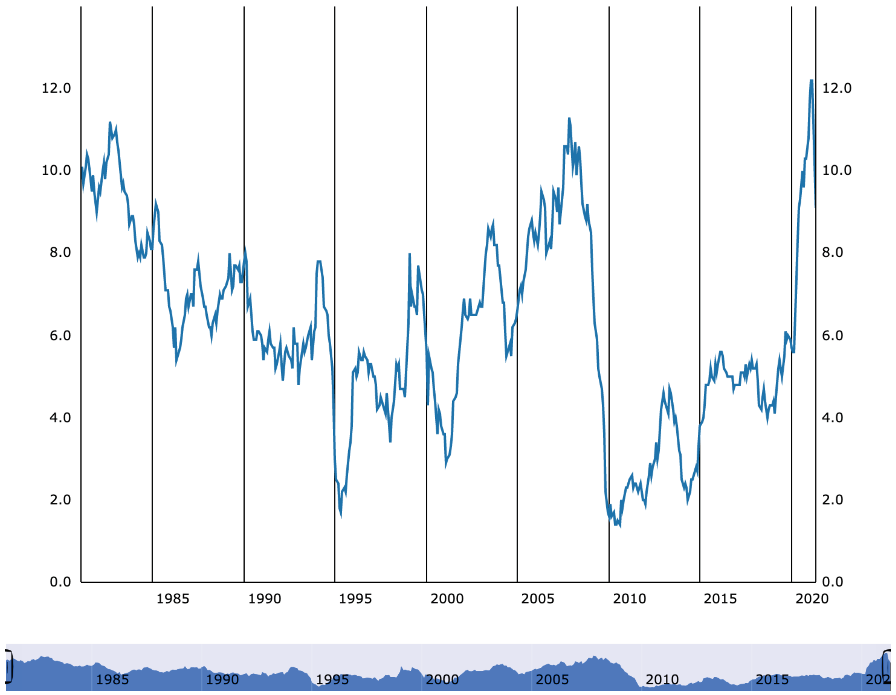
The choice of using the money stock growth as a driver for the first mode of the simulation was based on real-world observations. Indeed, looking at the data supplied by the statistical warehouse of the ECB1, the money stock (M22) in Europe has, although not smoothly, been on the rise over the last 4 decades (Figure 1). Although the growth rate of the money stock has not been constant (Figure 2), it has been bounded. An average growth rate was used in the simulations.
The second mode of the simulation was based on the assumption that an unbounded loan demand is unrealistic. A fixed loan ratio, a percentage relative to the money stock, was set to initialise this mode.
The computational model was initialised with the following parameters:
  • Growth mode:
    -
    g: growth rate of the money stock;
  • Loan demand mode:
    -
    L R : loan ratio expressed as a percentage of the current money stock;
  • Both modes:
    -
    C: number of cycles. Each cycle is interpreted as one year;
    -
    The initial state of all balance sheets;
    -
    Parameters for the bank sector:
    m: loan maturity;
    p: profit retention ratio on debt.
Variables tracked during the simulation:
  • t: cycle number;
  • M t : money stock;
  • D t : private debt held by the bank;
  • D R t = D t M t : debt ratio;
  • L t : size of the loan demand;
  • I t : instalment due.

4. Simulations

The goal of the following simulations was to determine the conditions under which the model remains stable. Assuming that an ever-rising D R is not feasible in a real-world economy, the stability of the model is defined as D R converging to a bounded value.
Initial M 0 is created with a loan L 0 . Every subsequent cycle, a new loan L t is created according to the parameters of the simulation mode. Loans are paid off over a period equal to their maturity m, resulting in m instalments i, which are all equal to L t m . In the text below, I t is used, being the sum of all i being due at cycle t. Loans that have reached their maturity are retired.
p does not necessarily correspond to real-world values. This is inconsequential for determining the properties of the model.
D R t is calculated.

4.1. Fixed Growth Rate

The following simulations assumed a fixed growth rate g:
  • t , M t M t 1 M t 1 = g
Each cycle, the following equations were processed:
  • M t a r g e t = ( 1 + g ) M t 1
  • D t = D t 1 I t
  • M t = M t 1 I t p D t 1
  • L t = M t a r g e t M t
  • M t M t + L t
  • D t D t + L t
The following output was analysed:
  • D R t = D t M t

4.1.1. Mathematical Analysis

For a fixed growth rate scenario, it is possible to derive an analytical solution for D R with a fixed growth rate g for M. This solution eliminates L from the equations.
From the balance sheet analysis, it can be concluded that M plus bank sector equity (E) equals D, expressed as continuous functions:
M ( t ) + E ( t ) = D ( t )
A fraction of M equal to p D is converted into E each cycle:
E ( t ) = E ( t 1 ) + D ( t 1 ) p
M grows by percentage g each cycle:
M ( t ) = M 0 ( 1 + g ) t
We can define:
D R ( t ) = D ( t ) M ( t )
D ( t ) = D R ( t ) M ( t )
E ( t ) = ( D R ( t ) 1 ) M ( t )
Substituting ( 5 ) and ( 6 ) in ( 2 ) gives us the recurrence relation for s ( t ) :
D R ( t ) = D R ( t 1 ) ( 1 + p ) p 1 + g + 1
the solution to which is:
D R ( t ) = p 1 + p 1 + g t g p g
Special cases:
g = 0 (no-growth scenario for M) D R ( t ) reduces to ( p + 1 ) t
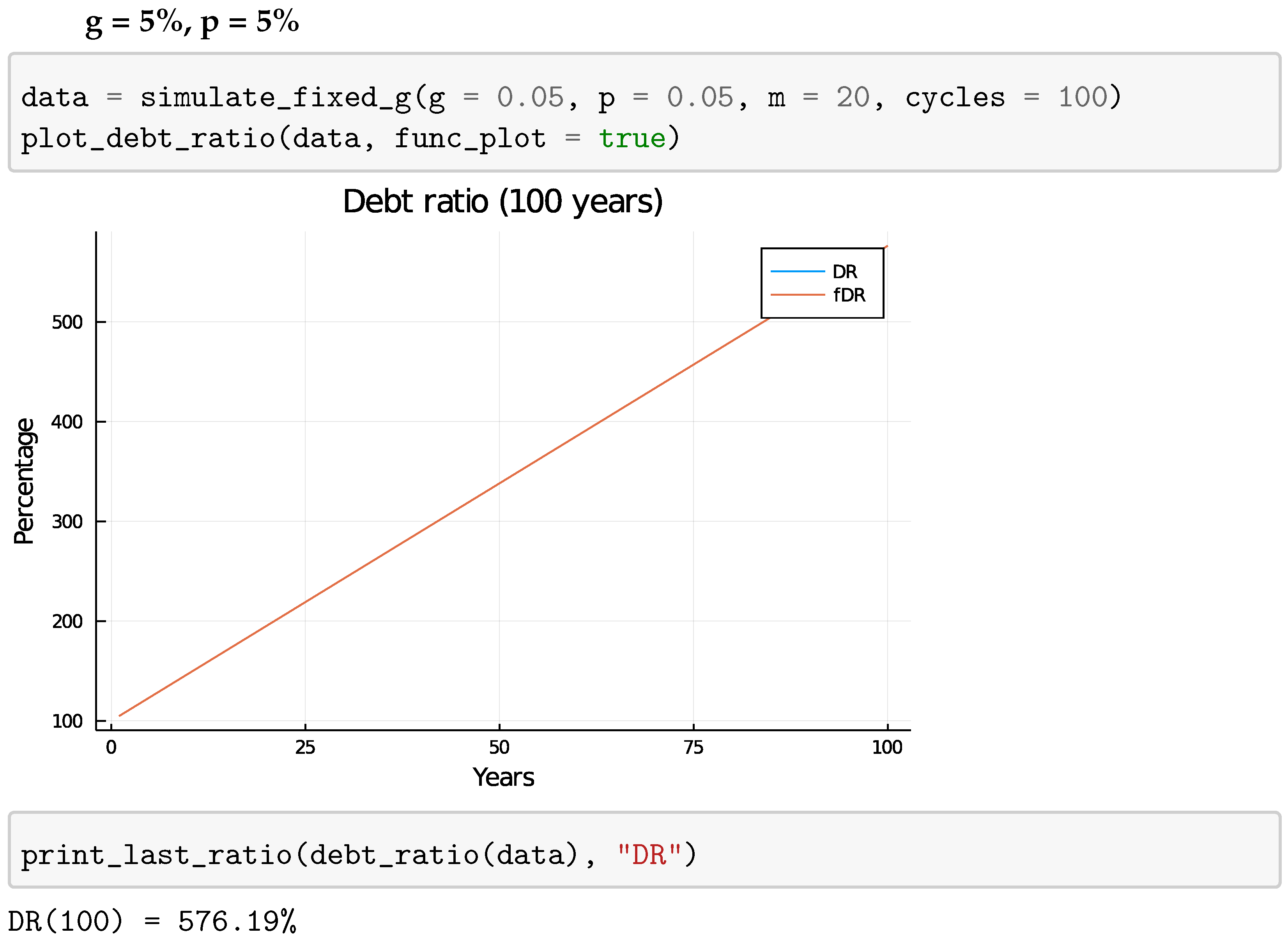
p = g lim p g D R ( t ) = g t 1 + g + 1
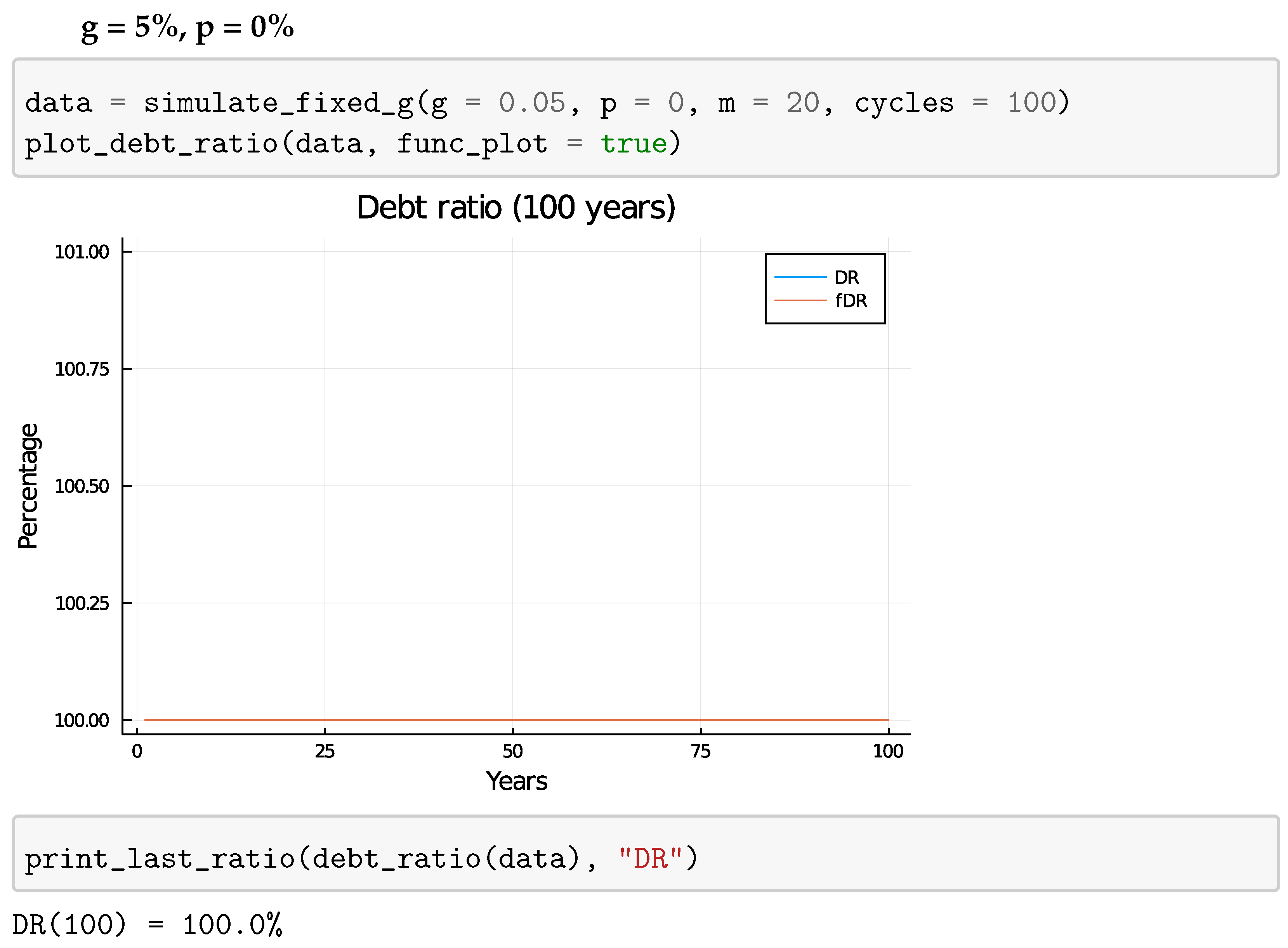
p = 0 (no profit retention) D R ( t ) = 1
p < g lim t inf D R ( t ) = g g p

4.1.2. Plots

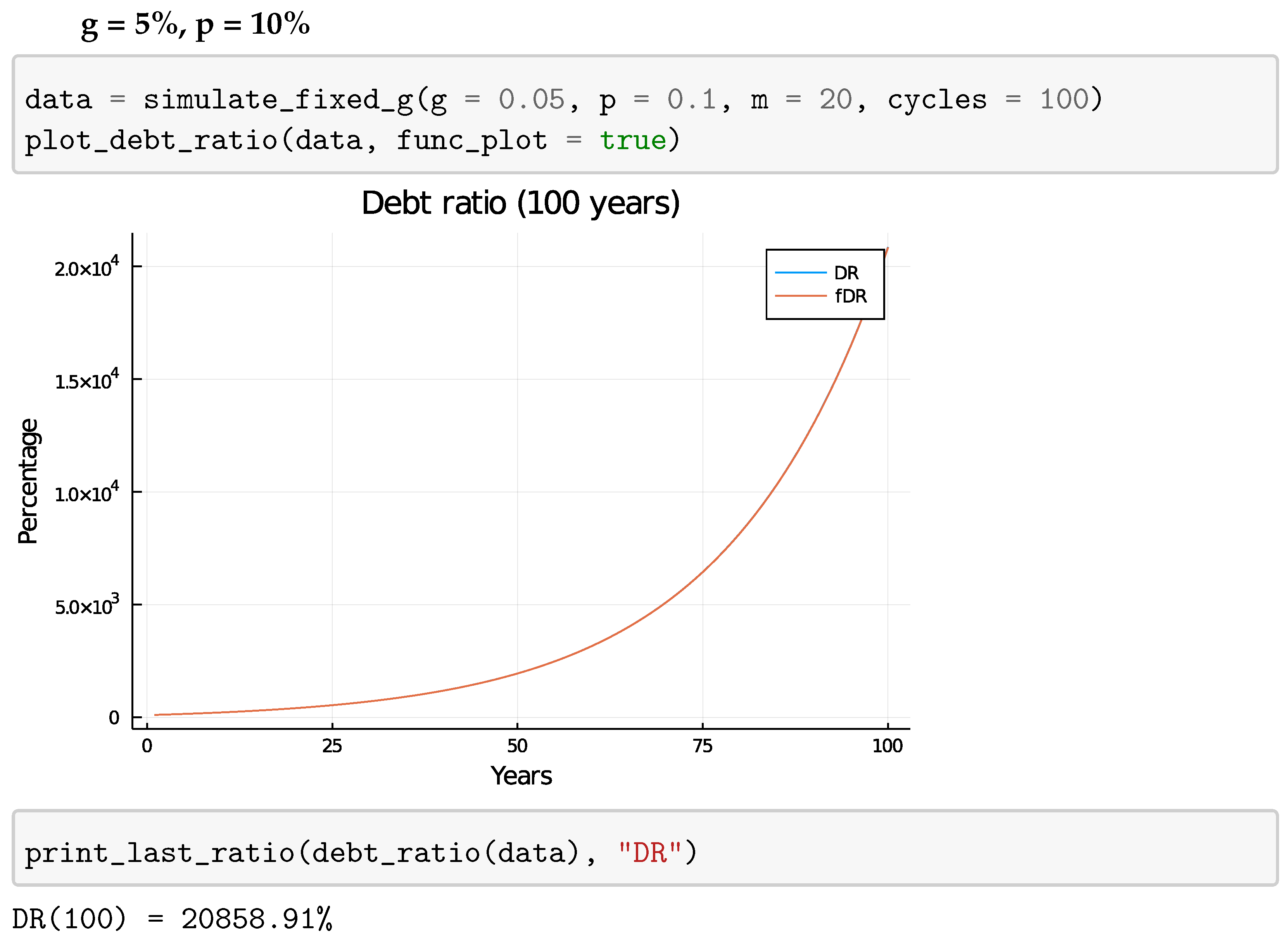
For each plot, the output from the mathematical functions is plotted as fDR alongside the output of the simulation for comparison (Figure 3, Figure 4, Figure 5, Figure 6 and Figure 7).

4.2. Fixed Loan Ratio

Although L can be mathematically factored out, g, which can be observed from real-world data, is the result of the balance among L, I and p D :
  • g t = M t 1 + L t I t p D t M t 1
The following simulations assumed a fixed L R :
  • t , L t M t = L R
  • M t = M t 1 I t p D t + L t
  • L t M t 1 I t p D t 1 + L t = L R
  • L t = L R ( M t 1 I t p D t 1 + L t )
  • L t = M t 1 ( I t + p D t 1 ) 1 L R L R
Each cycle, the following equations were processed:
  • L t = M t 1 ( I t + p D t 1 ) 1 L R L R
  • M t = M t 1 ( I t + p D t 1 ) + L t
  • D t = D t 1 I t + L t
The following output was analysed:
  • M t
  • g t = M t M t 1 M t 1
  • D R t = D t M t
I t is dependant on m, and therefore, L t will vary for different values of m. The effects were examined in the simulations.
The simulations stopped automatically when M t 0 . The effective runtime displayed equals the number of years where M t > 0 .

5. Discussion

5.1. Observations

5.1.1. Fixed Growth Rate

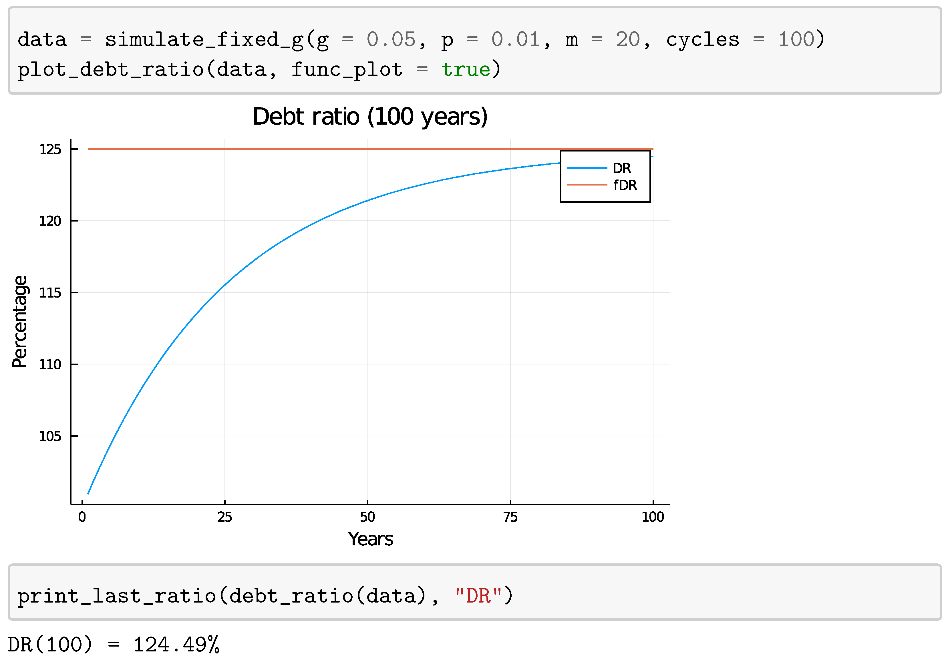
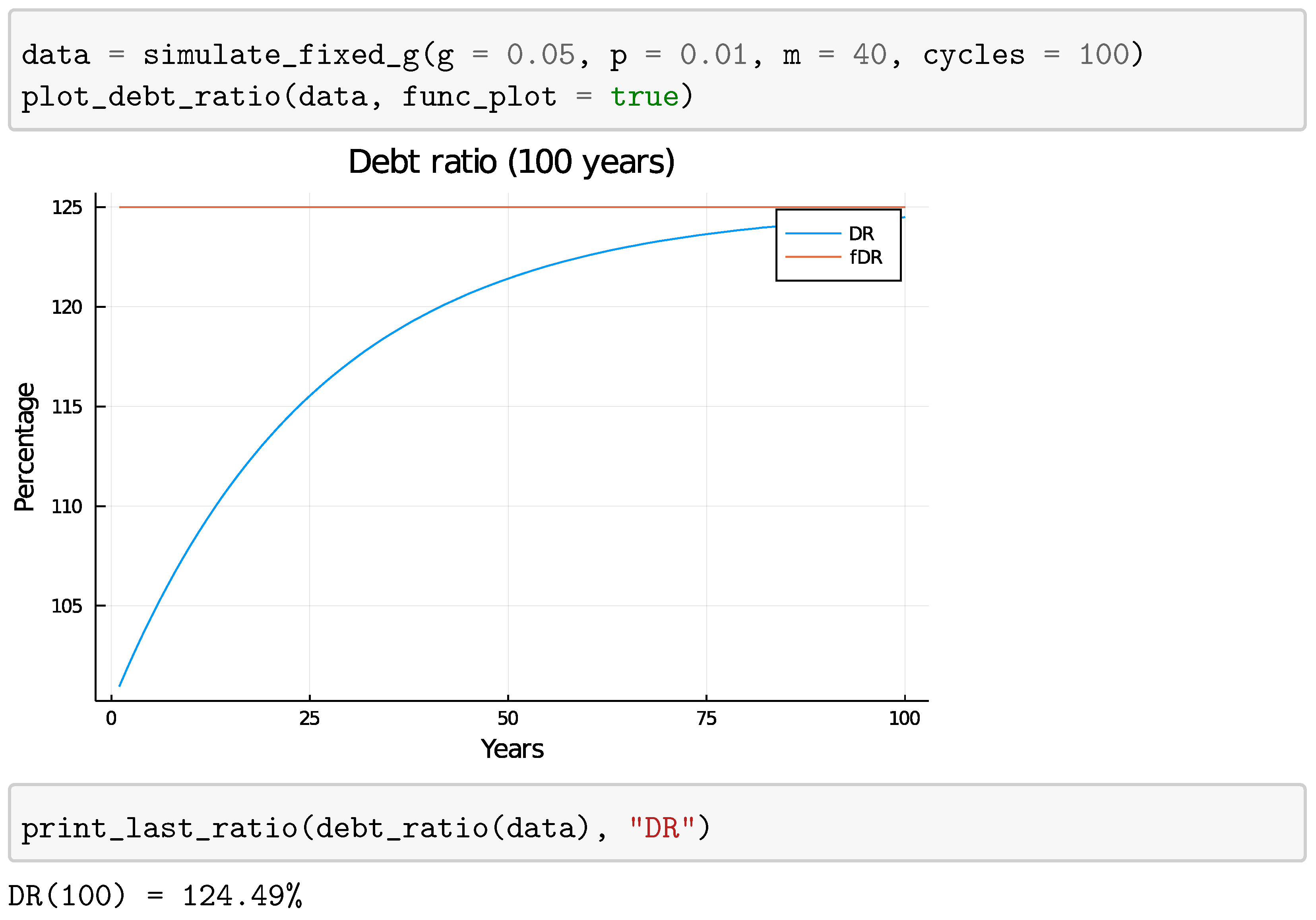
In the mathematical analysis, L was factored out. Therefore, loan maturity should have no effect on D R . Indeed, when the simulations were executed with different maturities, D R was unaffected (Figure 20 and Figure 21).
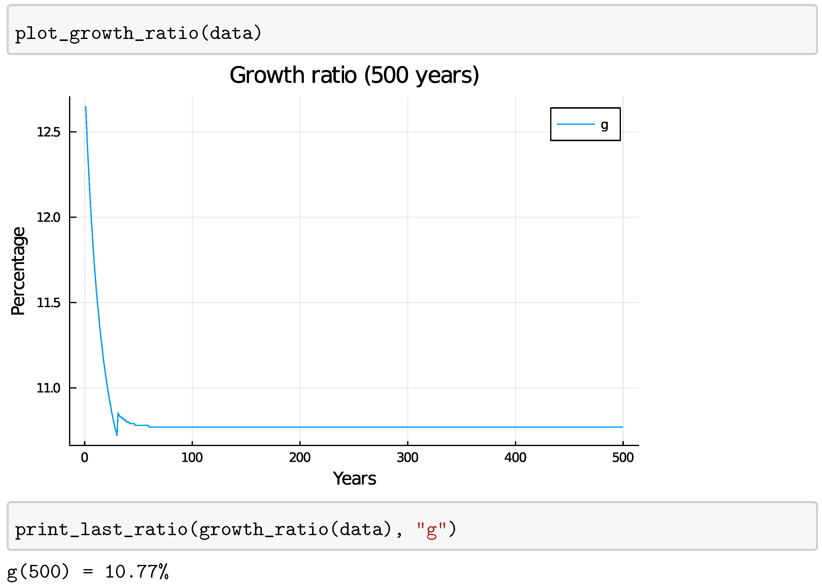
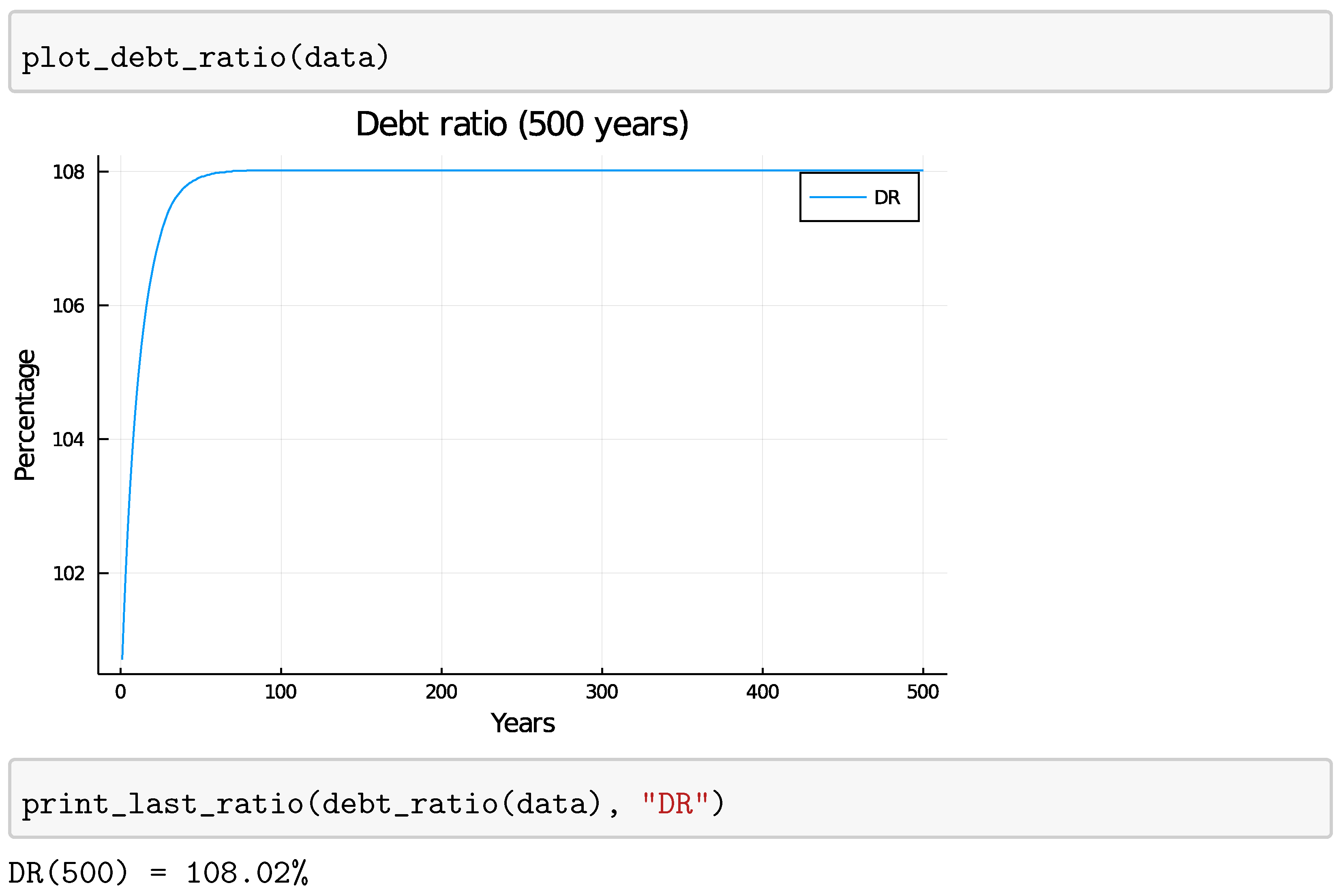
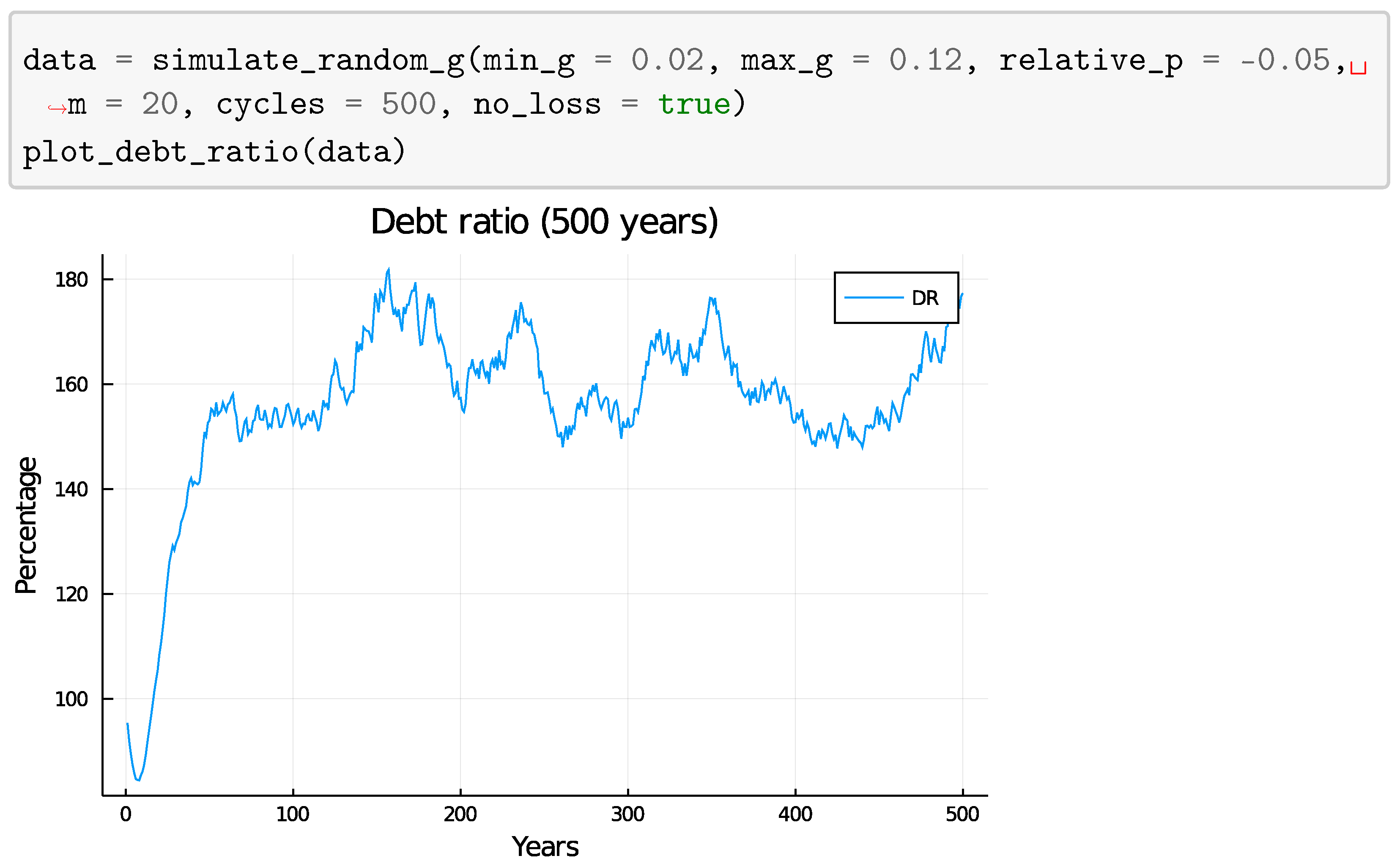
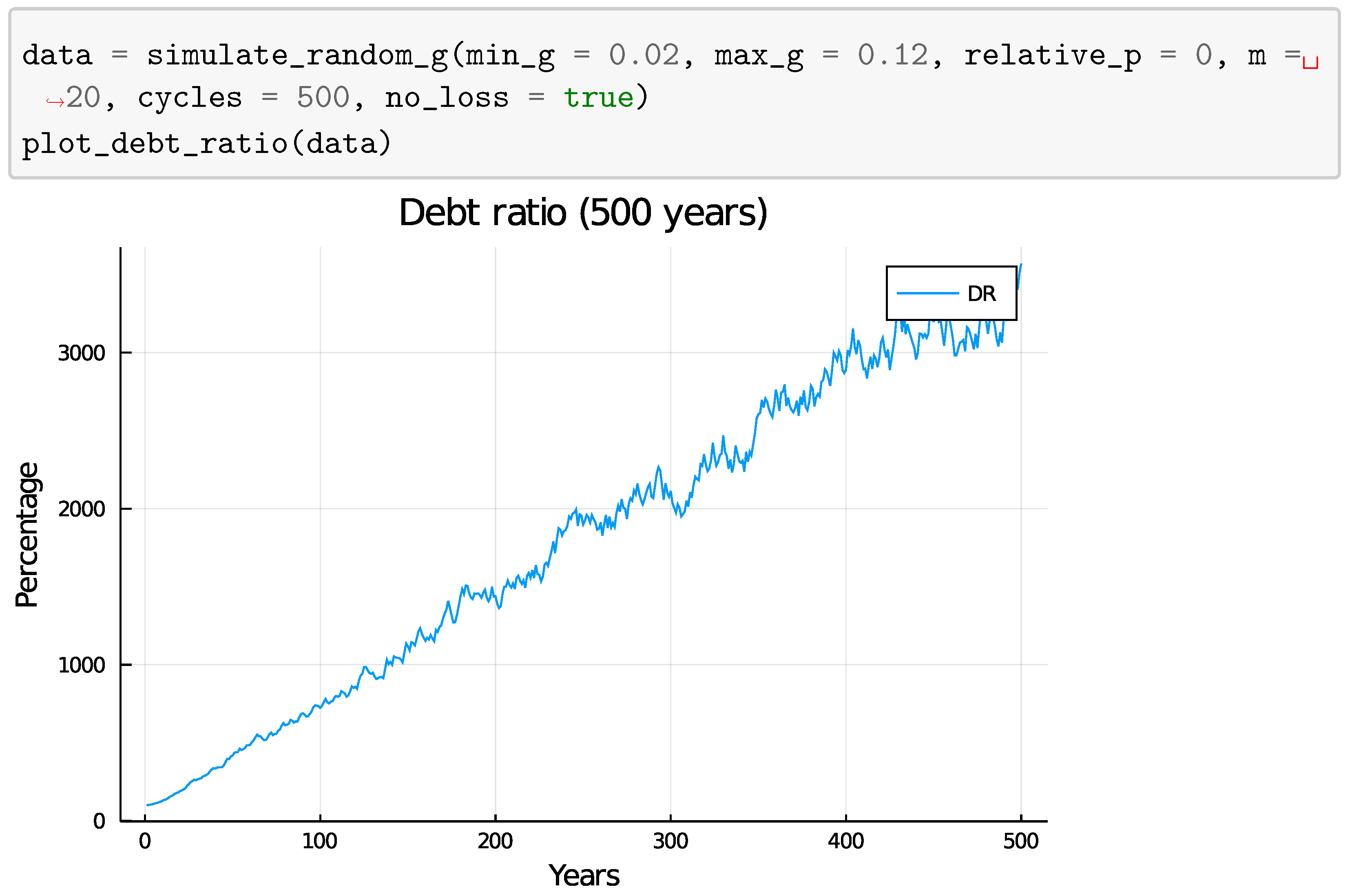
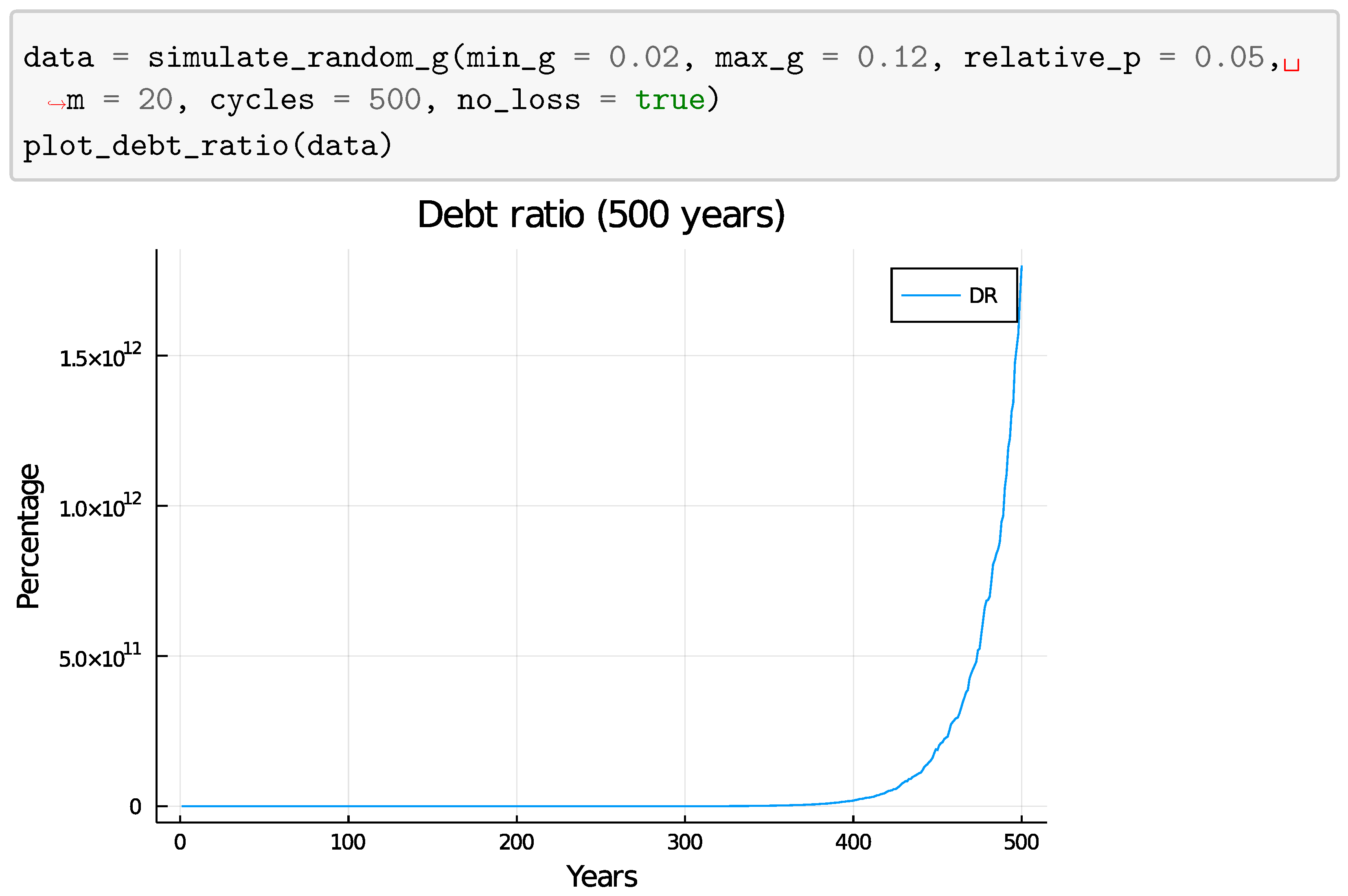
When g was fixed and as long as p < g , the model remained stable and D R converged to g g p . As soon as p g , D R no longer has an upper bound, thereby breaking the requirement for stability. This holds true even when g was determined randomly each cycle, within limited bounds, and p was set relative to this random g (Figure 22, Figure 23 and Figure 24). When the model was run with 2 % g 12 % , which are approximately the boundaries observed in Figure 2, variations in p, where p is either smaller, equal to or greater than g, resulted in trends similar to the simulations with a fixed g.
Very small differences between p and g led to results that seemed to deviate from the expectations, but that stemmed from D R being significantly higher, and therefore, in the simulations, it took longer before convergence occurred. This is shown in the mathematical analyses.
Since loans were the driving force in the simulations, they can also be used to calculate the resulting L R , which is the required L R for a given combination of p, g and m. L R follows the same pattern as D R and becomes unbounded when p g .

5.1.2. Fixed Loan Ratio

For parameters leading to a stable model, the results of fixed L R simulations can be fed into fixed growth simulations to produce the same results.
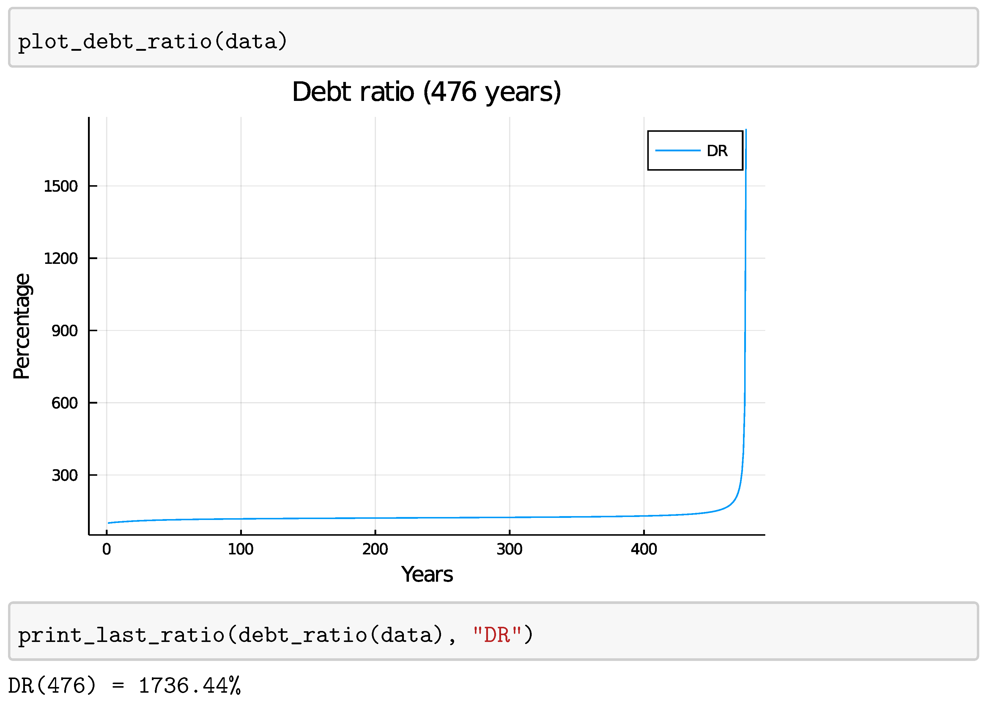
For example, feeding the result g = 4.75 % from L R = 15 % , p = 0.8 % (Figure 10) into a fixed g simulation resulted in the same result for D R , namely = 120.25% (Figure 25).

5.2. Steady-State Economy

It can clearly be stated that discussion about the possibility of a steady-state economy in conjunction with a debt-based, interest-bearing monetary system only makes sense if that monetary system is stable. The results from the simulations and the accompanying mathematical analyses therefore add a new perspective to the discussion.
Cahen-Fourot and Lavoie (Cahen-Fourot and Lavoie 2016) stated that, in order to have a steady-state economy, banks and organisations must not accumulate wealth, i.e., a portion of accumulated wealth should be spent, resulting in zero net wealth accumulation.
This was not contradicted by the simulations. Zero net wealth accumulation for banks would result in p = 0 , leading to a stable system g 0 . However, no definite conclusions can be reached about whether a steady-state economy can be reached since it is clear that the monetary system itself can be examined without taking economic parameters such as wages, production, consumption and private savings into account.
It is therefore suggested that the question about whether or not a post-Keynesian money supply model is inherently incompatible with a steady-state economy be restated as follows: Can a steady-state economy realistically support a stable post-Keynesian money supply model?
It was observed that the stability of the model is dependent on p < g . For this to happen, a minimal L R needs to exist. This minimal L R is dependent on the behaviour of the economic actors in the private sector. While, theoretically, p and m could be part of monetary policy, L R cannot.
If the position is taken that in a steady-state economy, businesses should be able to cover operating and depreciation costs with their revenues, then there is a high likelihood that sufficient L R would be lacking, leading to a negative g. This in turn would require the banking sector to operate at a loss in order to maintain stability, an event that is unlikely to occur.
The fact that the banking sector does not always answer positively to a loan demand puts additional strain on achieving the necessary L R .
Furthermore, if the balance sheet recession of Japan (Koo 2013) is any indication, things appear bleak. However, a declining M could be the incentive needed to raise L R , but more research would be required before stating definitive conclusions.
The behaviour of the economic actors—the private sector demanding loans and the banking sector approving loans and determining p—should be included in the model. Is the banking sector willing to subject p to g? Is the private sector willing to borrow sufficient amounts in order to satisfy the necessary L R ? Which are the underlying incentives that drive borrowing, and how strong are they in a steady-state economy?
The most heated discussions in the debate about whether or not an inherent growth imperative exists in debt-based, interest-bearing monetary systems seems to be rooted in the definition of “inherent growth imperative”. This definition is not the same for opposing sides of the argument. For those who claim there is no growth imperative, the real-world behaviour of the economic actors interacting with the monetary system is not taken into consideration when determining the existence of the growth imperative.
On the opposite side of the discussion, the necessary conditions for a steady-state economy—banks and organisations freely distributing their profits—are claimed to be unrealistic, and therefore, a steady state can not be reached when using a debt-based, interest-bearing monetary system.
Realistically, behaviour cannot merely be assumed to match the requirements of a mathematical model. Excluding real-world behaviour and the underlying incentives of the economic actors would make this behaviour external to the model and thereby result in money creation, driven by externalised behaviour, to lean towards exogeneity rather than endogeneity, thereby undermining the endogenous character of post-Keynesian money supply models. The articles from the literature study stating the absence of a growth imperative in a post-Keynesian money supply model all assumed that the behaviour of the economic actors falls in line with the needs of the model, but no supportive arguments for the validity of these assumptions were made.

5.3. Green Economy

The debate about whether or not debt-based, interest-bearing monetary systems demand a growing economy needs to be interpreted as part of a broader discussion about the sustainability of our current economic growth model. The degrowth movement3 argues that the growth model must be abandoned, while growth proponents propose a green growth model that allows economic growth while at the same time reducing resource usage and abating the negative impacts on climate and biodiversity.
While most economists from both sides agree that action needs to be undertaken in order to mitigate the effects of resource extraction and waste disposal on our living environment, there is disagreement on the severity of the measurements that are necessary. Proponents of green growth (OECD 2011, 2012; Bowen and Hepburn 2014) advocate that economic growth is needed in order to maintain prosperity and to lift people in developing countries out of poverty. Opponents state that sustained economic growth cannot go hand in hand with a reduced impact on our environment and that new models for well being and prosperity need to be developed (Hickel and Kallis 2019; Parrique et al. 2019).
Even though the debate is still ongoing, it seems that openness for a reconsideration of our economic growth model is on the rise (D’Alessandro et al. 2020; OECD 2020). This might in part have to do with the complexity of achieving a green growth model. Implementing green growth is not a straightforward endeavour. A combination of adequate accounting methods, political will to implement green policies, which often come with a cost over the short term, and economic incentives for green investments is needed (Batrancea et al. 2020; Dogaru 2021; Hallegatte et al. 2012; Hepburn et al. 2018; Kingsley 2017; Larissa et al. 2020; Nordhaus 2015; Ozili 2021).

5.4. Inflation/Deflation

Although inflation and deflation have no direct effect on the model, they influence L R . Continuous inflation makes sure the nominal size of loans—for the same purchases—rises with time, thereby helping to prop up g. Should deflation occur, nominal loan size would diminish, thereby putting a downward strain on L R and, as a consequence, also on g. Therefore, deflation would put the stability of the model at risk. This might be a reason why central banks vie to maintain positive inflation ratios.

5.5. Model Limitations

The destabilised outcomes of the presented simulations do not unfold themselves in the real economy today.
This indicates that either p < g or that other elements, missing from the model, are responsible for avoiding a collapse. What follows is a brief overview of those elements that could restore balance to the model.

5.5.1. Quantitative Easing

Quantitative easing (QE), which has been applied extensively by central banks during the COVID-19 pandemic, increases M without resulting in increased debt. This reduces the D M ratio and also lowers the required L R , thereby reducing stress on the model. However, when the debt is settled or it is cleared from the balance sheets of central banks by reselling it to the financial markets, the reverse would happen. M would decrease and increase stress on the model.

5.5.2. Government Spending

Government spending can, under certain conditions, alleviate stress from the model.
When the government can spend money into existence, as claimed by MMT advocates (Kelton 2020), M can be increased in order to alleviate stress from the model. Decreasing M through taxation holds the same risks, as reselling debt bought up through QE would do, namely to increase stress on the model. M decreases while D remains the same, thereby raising D R .
In case the government cannot spend money into existence, they either have to borrow it from the private sector by issuing bonds or borrow it from banks.
When money is borrowed by issuing bonds and that money is then spent, no effects on the model occur. Money has moved from private investors to the government and back to private actors who are paid by the government. Both private investors and actors paid by the government are part of the private sector, and M does not change.
When the government borrows from a bank and then spends that money it has the same effect as a private actor making a bank loan.
Should governments hold on to money they borrowed, it can be considered to be the same as accumulated wealth, i.e., “dead” money.

5.5.3. Banks Selling Debt at a Loss

If banks were to sell their debt to the financial market at a loss, this would effectively create “debtless money” from credit money. Consider the following balance sheets to be the initial state:
Bank balance sheet:
AssetsLiabilities
Private debt = 100,000Deposits = 80,000
Equity = 20,000
Private sector balance sheet:
AssetsLiabilities
Deposits = 80,000Private debt to bank = 100,000
Equity = −20,000
If the bank were to sell 20,000 of its private debt for 15,000, renaming it as a security, the resulting balance sheets would look like this:
Bank balance sheet:
AssetsLiabilities
Private debt = 80,000Deposits = 65,000
 Equity = 15,000
Private sector balance sheet:
AssetsLiabilities
Deposits = 65,000Private debt to bank = 80,000
Security = 20,000Private debt to investor = 20,000
 Equity = −15,000
The equity of the bank has been lowered by 5000, and private sector equity has risen by an equal amount. From the perspective of systemic stability, it does not matter that the debt is ever settled. Settlement of a debt held by private actors merely moves money around instead of destroying it, which is the case when a bank debt is paid off.
This process lowers D M from 125% to 123.08%, thereby alleviating stress from the model. Banks selling debt at a loss is beneficial for the stability of the model. It is even better for the long-term stability of the model when compared to QE and government spending because it essentially lowers p and no trivial reverse process exists.
The solvency of banks would however be jeopardised should they lose more than they hold in equity.

5.5.4. Loan Defaulting

When private actors default on their loans, a process similar to selling debt as a loss occurs. In this case, the loss incurred by the bank equals the value of the loan minus the price for which they can sell claimed assets.
This is beneficial for the long-term stability of the model.

6. Conclusions

A common definition of the systemic boundaries of post-Keynesian money supply systems is needed in order to be able to settle the argument about the existence of an inherent growth imperative in those systems.
The economic actors and their real-world behaviour and underlying incentives should be considered as an integral part of the monetary system. An endogenous money supply can simply not exist without a loan demand coming from the economic actors. Even the model presented here would not generate a money supply without this demand. Therefore, it can be stated that a debate about intrinsic growth imperatives without the inclusion of economic actors and their real-world behaviour makes little sense.
A restatement of the inherent growth imperative research question is suggested. Can a steady-state economy realistically support a stable post-Keynesian money supply model (stability being defined as having a bounded debt ratio ( D R ))? This requires extensive behavioural research on simulated steady-state economies.
The model observations make it clear that stability can only be achieved when the net profit ratio of the aggregate bank (p), relative to their debt assets (D), is less than the growth rate (g) of the money supply (M). The implication of this condition is that there must exist an adequate loan ratio ( L R ) and thus an adequate loan demand from the private sector.
These observations cannot be easily disregarded. Under the assumption that the post-Keynesian money supply theory is correct, the dynamics presented here must be at play. They are inherent to any debt-based monetary system where banks make a profit. Events such as QE, loan defaulting and banks selling off loans at a loss counter destabilisation by artificially boosting g and/or lowering p, but the frequency and circumstances that cause these should be investigated further. It would therefore be interesting to revisit the analysis of systemic banking crises (Laeven and Valencia 2018) and the use of unconventional balance sheet policies (Stone et al. 2011), both performed by the IMF, with this information in mind.
This can be seen as an opportunity to contemplate pragmatic action towards a green economy. Although definite answers on a growth imperative remain illusive, there is a strong indication that a sufficient L R might not be achievable in a steady-state economy. Should the implementation of a green growth economy prove to be impossible or inadequate, it would mean that either the current system must be permanently modified in order to ensure that p < g or the transition to a new monetary system must be prepared. It might therefore be wise to spend more effort on alternatives for both the current economic growth model and debt-based, interest-bearing monetary systems.
From the perspective of scientific rigour and prudence towards changing large-scale systems, it is preferable to arrive at definite answers before taking action. Considering the complexity of the economic system as a whole, combined with the equally complex topic of incentive-driven behaviour, this is a daunting task, especially since time is also an issue. Climate reports have become increasingly alarming (IPCC 2018, 2019a, 2019b), and at the UN conference of 20194, it was claimed there were only 11 years left to turn the tide on climate change. Pragmatic, innovative and experimental approaches such as using large-scale game simulations (Li et al. 2021; Ramsey and Renault 2020) could provide a solution.

Author Contributions

Conceptualization: S.K.; methodology: S.K. (computational) and T.G. (math); software: S.K.; validation: S.K., T.G and B.D.; formal analysis: S.K. (computational) and T.G. (math); investigation: S.K.; resources: S.K.; writing—original draft preparation: S.K.; writing—review and editing: T.G and B.D.; visualisation: S.K.; supervision: S.K.; project administration: S.K. All authors have read and agreed to the published version of the manuscript.

Funding

This research received no external funding.

Institutional Review Board Statement

Not applicable.

Informed Consent Statement

Not applicable.

Data Availability Statement

Conflicts of Interest

The authors declare no conflict of interest.

Appendix A. Source Code

The source code for the model was implemented in Julia and is Available online: https://github.com/HapponomyOrg/MoneySim.jl (accessed on 2 July 2021).
The source code uses the EconoSim.jl v0.2.0 package, which is available at: https://github.com/HapponomyOrg/EconoSim.jl (accessed on 2 July 2021).

Notes

1
Eurostat website: https://sdw.ecb.europa.eu (accessed on 13 June 2021).
2
Since cash is not used in the model, M2 is not exactly the same as M, but it is the closest real-world measurement to it.
3
https://www.degrowth.info/en/ (accessed on 13 July 2021).
https://degrowth.org (accessed on 13 July 2021).
4
UN Meeting Coverage. Only 11 Years Left to Prevent Irreversible Damage from Climate Change, Speakers Warn during General Assembly High-Level Meeting. https://www.un.org/press/en/2019/ga12131.doc.htm (accessed on 13 July 2021).

References

  1. Arnsperger, Christian, Jem Bendell, and Matthew Slater. 2021. Monetary Adaptation to Planetary Emergency: Addressing the Monetary Growth Imperative. Ambleside, UK: University of Cumbria, Available online: https://insight.cumbria.ac.uk/id/eprint/5993 (accessed on 13 July 2021).
  2. Banerjee, Abhijit V., and Eric S. Maskin. 1996. A Walrasian Theory of Money and Barter. The Quarterly Journal of Economics 111: 955–1005. [Google Scholar] [CrossRef] [Green Version]
  3. Batrancea, Ioan, Larissa Batrancea, Malar Maran Rathnaswamy, Horia Tulai, Gheorghe Fatacean, and Mircea-Iosif Rus. 2020. Greening the Financial System in USA, Canada and Brazil: A Panel Data Analysis. Mathematics 8: 2217. [Google Scholar] [CrossRef]
  4. Bowen, Alex, and Cameron Hepburn. 2014. Green growth: An assessment. Oxford Review of Economic Policy 30: 407–22. [Google Scholar] [CrossRef]
  5. Bundesbank, Deutsche. 2017. The role of banks, nonbanks and the central bank in the money creation process. Monthly Report 69: 13–34. [Google Scholar]
  6. Cahen-Fourot, Louison, and Marc Lavoie. 2016. Ecological monetary economics: A post-Keynesian critique. Ecological Economics 126: 163–68. [Google Scholar] [CrossRef]
  7. Caiani, Alessandro, Antoine Godin, Eugenio Caverzasi, Mauro Gallegati, Stephen Kinsella, and Joseph E. Stiglitz. 2016. Agent based-stock flow consistent macroeconomics: Towards a benchmark model. Journal of Economic Dynamics and Control 69: 375–408. [Google Scholar] [CrossRef] [Green Version]
  8. D’Alessandro, Simone, André Cieplinski, Tiziano Distefano, and Kristofer Dittmer. 2020. Feasible alternatives to green growth. Nature Sustainability 3: 329–35. [Google Scholar] [CrossRef]
  9. Dogaru, Lucreția. 2021. Green Economy and Green Growth—Opportunities for Sustainable Development. Paper presented at the 14th International Conference on Interdisciplinarity in Engineering—INTER-ENG 2020, Târgu Mureș, Romania, October 8–9. [Google Scholar]
  10. Farley, Joshua, Matthew Burke, Gary Flomenhoft, Brian Kelly, D. Forrest Murray, Stephen Posner, Matthew Putnam, Adam Scanlan, and Aaron Witham. 2013. Monetary and Fiscal Policies for a Finite Planet. Sustainability 5: 2802. [Google Scholar] [CrossRef] [Green Version]
  11. Godley, Wynne, and Marc Lavoie. 2012. Monetary Economics. London: Palgrave Macmillan. [Google Scholar] [CrossRef]
  12. Godley, Wynne. 2004. Towards a Reconstruction of Macroeconomics Using a Stock Flow Consistent (SFC) Model. University of Cambridge: Available online: https://www.repository.cam.ac.uk/bitstream/handle/1810/225167/wp16.pdf;jsessionid=90B9B20A5C98CDBF38CA6F162D785CAE?sequence=1 (accessed on 13 July 2021).
  13. Gross, Mr Marco, and Christoph Siebenbrunner. 2019. Money Creation in Fiat and Digital Currency Systems. IMF Working Papers Volume 2019, Issue 285. Available online: https://www.elibrary.imf.org/view/journals/001/2019/285/001.2019.issue-285-en.xml (accessed on 13 July 2021).
  14. Hallegatte, Stéphane, Geoffrey Heal, Marianne Fay, and David Treguer. 2012. From Growth to Green Growth—A Framework (No. w17841). Cambridge: National Bureau of Economic Research. [Google Scholar] [CrossRef]
  15. Hepburn, Cameron, Alexander Pfeiffer, and Alexander Teytelboym. 2018. Green Growth—Oxford Handbooks. In The New Oxford Handbook of Economic Geography. Oxford: Oxford University Press, p. 27. [Google Scholar] [CrossRef]
  16. Hickel, Jason, and Giorgos Kallis. 2019. Is Green Growth Possible? New Political Economy 25: 469–86. [Google Scholar] [CrossRef]
  17. IPCC. 2018. Special Report—Global Warming of 1.5 °C. Available online: https://www.ipcc.ch/sr15/ (accessed on 13 July 2021).
  18. IPCC. 2019a. Special Report—Climate Change and Land. Available online: https://www.ipcc.ch/srccl/ (accessed on 13 July 2021).
  19. IPCC. 2019b. Special Report—The Ocean and Cryosphere in a Changing Climate. Available online: https://www.ipcc.ch/srocc/ (accessed on 13 July 2021).
  20. Jackson, Tim, and Peter A. Victor. 2015. Does credit create a ‘growth imperative’? A quasi-stationary economy with interest-bearing debt. Ecological Economics 120: 32–48. [Google Scholar] [CrossRef]
  21. Kelton, Stephanie. 2020. The Deficit Myth: Modern Monetary Theory and How to Build a Better Economy. London: John Murray. [Google Scholar]
  22. Kingsley, Kelly Mua. 2017. Green Financing. SSRN Electronic Journal. Available online: https://papers.ssrn.com/sol3/papers.cfm?abstract_id=2940765 (accessed on 13 July 2021).
  23. Kinsella, Stephen, and Terence O’Shea. 2011. Solution and Simulation of Large Stock Flow Consistent Monetary Production Models Via the Gauss Seidel Algorithm. SSRN Journal. Available online: https://papers.ssrn.com/sol3/papers.cfm?abstract_id=1729205 (accessed on 13 July 2021). [CrossRef]
  24. Koo, Richard C. 2013. Balance sheet recession as the ‘other half’ of macroeconomics. European Journal of Economics and Economic Policies 10: 136–57. [Google Scholar] [CrossRef]
  25. Laeven, Mr Luc, and Mr Fabian Valencia. 2018. Systemic Banking Crises Revisited. IMF Working Papers 18. Washington: IMF. [Google Scholar] [CrossRef]
  26. Larissa, Batrancea, Rathnaswamy Malar Maran, Batrancea Ioan, Nichita Anca, Rus Mircea-Iosif, Tulai Horia, Fatacean Gheorghe, Masca Ema Speranta, and Morar Ioan Dan. 2020. Adjusted Net Savings of CEE and Baltic Nations in the Context of Sustainable Economic Growth: A Panel Data Analysis. Journal of Risk and Financial Management 13: 234. [Google Scholar] [CrossRef]
  27. Lavoie, Marc, and Wynne Godley. 2002. Kaleckian Models of Growth in a Coherent Stock-Flow Monetary Framework: A Kaldorian View. Journal of Post Keynesian Economics 24: 277–311. Available online: http://www.levyinstitute.org/pubs/Lavoie%20Godley_2001-02.pdf (accessed on 13 July 2021). [CrossRef]
  28. Li, Zhi, Po-Hsuan Lin, Si-Yuan Kong, Dongwu Wang, and John Duffy. 2021. Conducting large, repeated, multi-game economic experiments using mobile platforms. PLoS ONE 16: e0250668. [Google Scholar] [CrossRef] [PubMed]
  29. Lietaer, Bernard, Christian Arnsperger, Sally Goerner, and Stefan Brunnhuber. 2012. Money—Sustainability: The Missing Link. Devon: Triarchy Press, Available online: https://www.researchgate.net/publication/271506661_Money_and_sustainability_the_missing_link_a_report_from_the_Club_of_Rome_-_EU_Chapter_to_Finance_Watch_and_the_World_Business_Academy (accessed on 13 July 2021).
  30. McLeay, Michael, Amar Radia, and Ryland Thomas. 2014. Money Creation in the Modern Economy. London: Bank of England, Available online: https://www.bankofengland.co.uk/-/media/boe/files/quarterly-bulletin/2014/money-creation-in-the-modern-economy.pdf?la=en&hash=9A8788FD44A62D8BB927123544205CE476E01654 (accessed on 13 July 2021).
  31. Nayan, Sabri, Norsiah Kadir, Mat Saad Abdullah, and Mahyudin Ahmad. 2013. Post Keynesian Endogeneity of Money Supply: Panel Evidence. Procedia Economics and Finance 7: 48–54. [Google Scholar] [CrossRef] [Green Version]
  32. Nikiforos, Michalis, and Gennaro Zezza. 2017. Stock-Flow Consistent Macroeconomic Models: A Survey. Annandale-On-Hudson: Levy Economics Institute, Available online: https://www.levyinstitute.org/pubs/wp_891.pdf (accessed on 13 July 2021).
  33. Nordhaus, William. 2015. Climate Clubs: Overcoming Free-riding in International Climate Policy. American Economic Review 105: 1339–70. [Google Scholar] [CrossRef] [Green Version]
  34. OECD. 2011. Towards Green Growth. Available online: https://www.oecd.org/greengrowth/48012345.pdf (accessed on 13 July 2021).
  35. OECD. 2012. OECD Environmental Outlook to 2050: The Consequences of Inaction, Paris, Organization for Economic Cooperation and Development. Available online: https://www.oecd.org/g20/topics/energy-environment-green-growth/oecdenvironmentaloutlookto2050theconsequencesofinaction.htm (accessed on 13 July 2021).
  36. OECD. 2020. Beyond Growth: Towards a New Economic Approach, New Approaches to Economic Challenges. Paris: OECD. [Google Scholar] [CrossRef]
  37. Ozili, Peterson K. 2021. Digital Finance, Green Finance and Social Finance: Is There a Link? Available online: https://papers.ssrn.com/sol3/papers.cfm?abstract_id=3786881 (accessed on 13 July 2021).
  38. Parrique, Timothée, Barth Jonathan, Briens François, Kerschner Christian, Kraus-Polk Alejo, Kuokkanen Anna, and Spangenberg Joachim H. 2019. Decoupling Debunked: Evidence and Arguments Against Green Growth as a Sole Strategy for Sustainability. Brussels: European Environmental Bureau, Available online: https://eeb.org/library/decoupling-debunked/ (accessed on 13 July 2021).
  39. Ramsey, David M., and Jérôme Renault, eds. 2020. Advances in Dynamic Games: Games of Conflict, Evolutionary Games, Economic Games, and Games Involving Common Interest, Annals of the International Society of Dynamic Games. Cham: Springer International Publishing. [Google Scholar] [CrossRef]
  40. Richters, Oliver, and Andreas Siemoneit. 2017. Consistency and stability analysis of models of a monetary growth imperative. Ecological Economics 136: 114–25. [Google Scholar] [CrossRef] [Green Version]
  41. Stone, Mark R., Kenji Fujita, and Ishi Kotaro. 2011. Should Unconventional Balance Sheet Policies Be Added to the Central Bank toolkit? a Review of the Experience so Far; IMF Working Papers 11. Washington: IMF. Available online: https://www.imf.org/external/pubs/ft/wp/2011/wp11145.pdf (accessed on 13 July 2021).
  42. Werner, Richard A. 2014. Can banks individually create money out of nothing?—The theories and the empirical evidence. International Review of Financial Analysis 36: 1–19. [Google Scholar] [CrossRef] [Green Version]
  43. Werner, Richard A. 2016. A lost century in economics: Three theories of banking and the conclusive evidence. International Review of Financial Analysis 46: 361–79. [Google Scholar] [CrossRef] [Green Version]
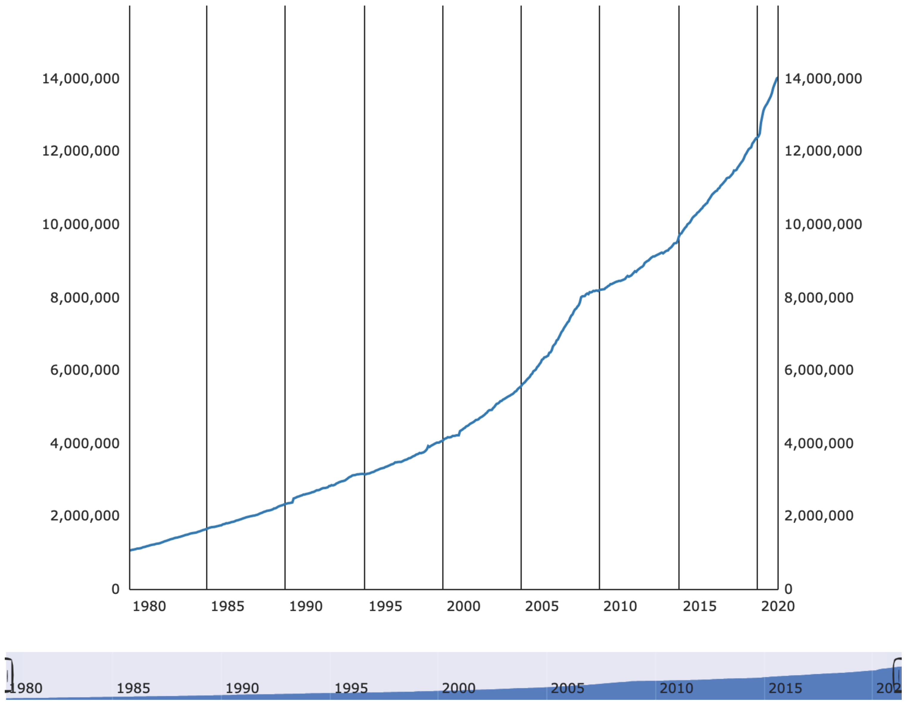
Figure 1. M2 Europe.
Jrfm 14 00335 g001
Figure 2. M2 growth Europe.
Jrfm 14 00335 g002
Figure 3. Debt ratio (g = 0%, p = 0%).
Jrfm 14 00335 g003
Figure 4. Debt ratio (g = 5%, p = 0%).
Jrfm 14 00335 g004
Figure 5. Debt ratio (g = 5%, p = 1%).
Jrfm 14 00335 g005
Figure 6. Debt ratio (g = 5%, p = 5%).
Jrfm 14 00335 g006
Figure 7. Debt ratio (g = 5%, p = 10%).
Jrfm 14 00335 g007
Figure 8. Money stock (LR = 15%, p = 0.8%, m = 20 years).
Jrfm 14 00335 g008
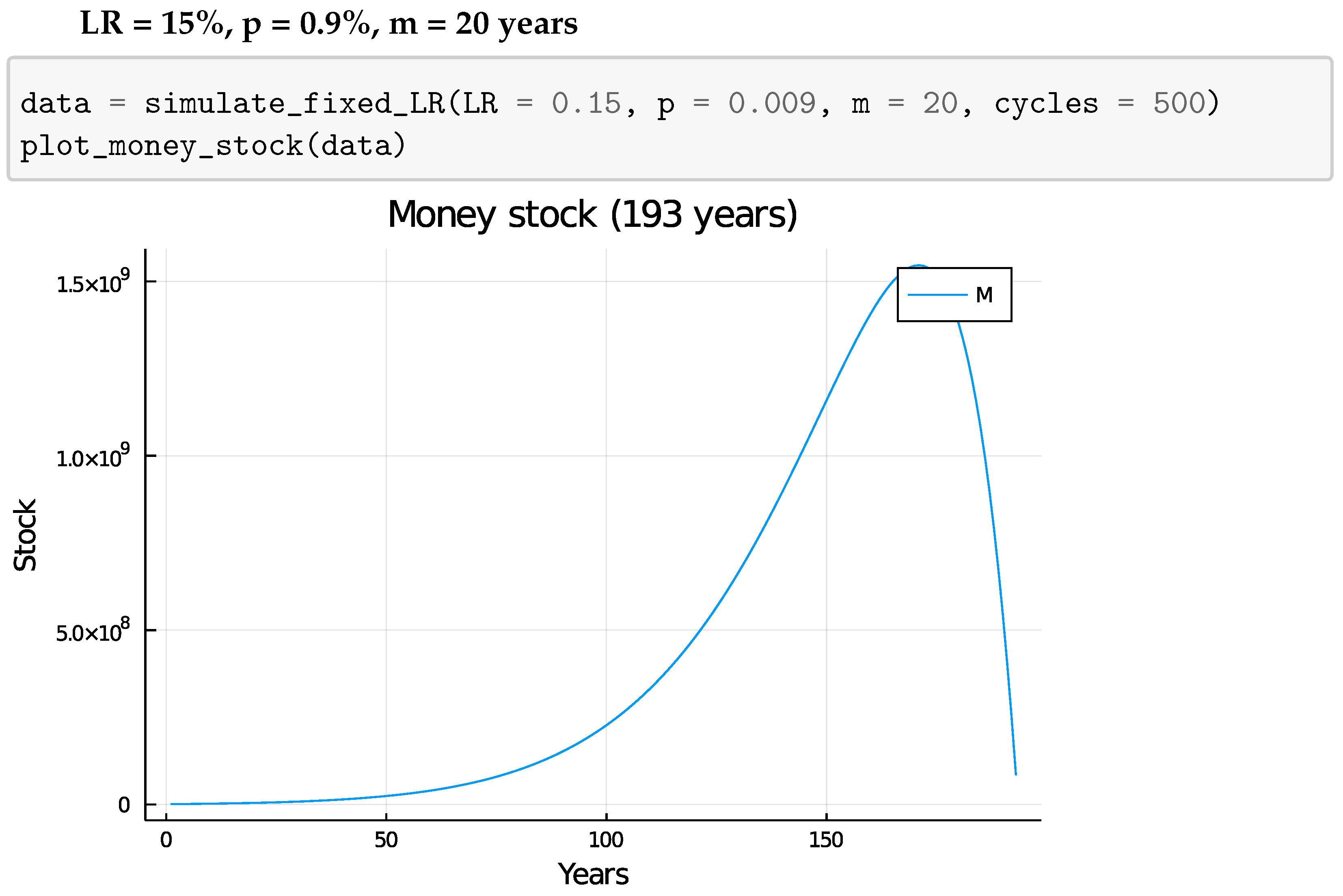
Figure 9. Growth ratio (LR = 15%, p = 0.8%, m = 20 years).
Jrfm 14 00335 g009
Figure 10. Debt ratio (LR = 15%, p = 0.8%, m = 20 years).
Jrfm 14 00335 g010
Figure 11. Money stock (LR = 15%, p = 0.9%, m = 20 years).
Jrfm 14 00335 g011
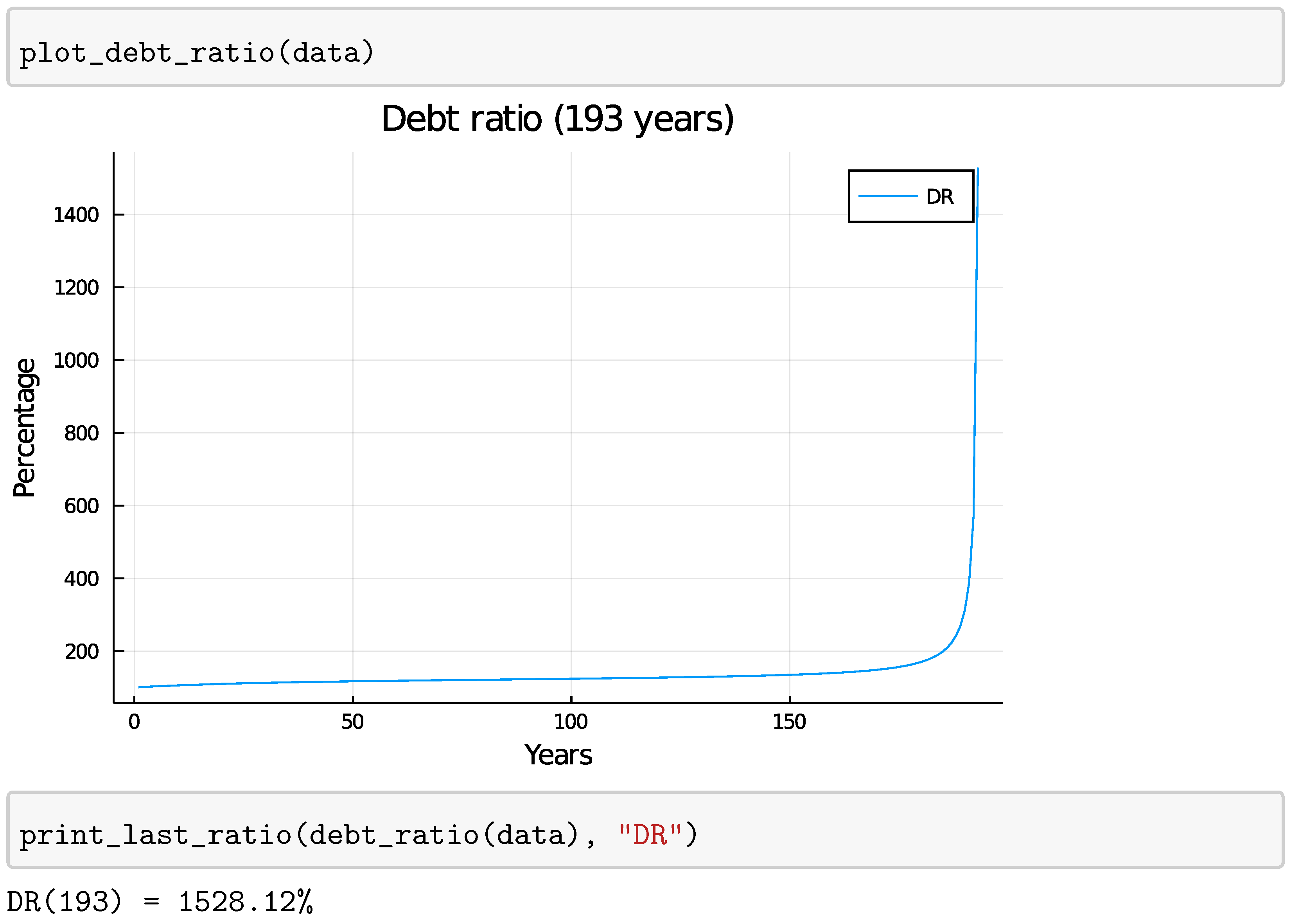
Figure 12. Growth ratio (LR = 15%, p = 0.9%, m = 20 years).
Jrfm 14 00335 g012
Figure 13. Debt ratio (LR = 15%, p = 0.9%, m = 20 years).
Jrfm 14 00335 g013
Figure 14. Money stock (LR = 14.9%, p = 0.8%, m = 20 years).
Jrfm 14 00335 g014
Figure 15. Growth ratio (LR = 14.9%, p = 0.8%, m = 20 years).
Jrfm 14 00335 g015
Figure 16. Debt ratio (LR = 14.9%, p = 0.8%, m = 20 years.
Jrfm 14 00335 g016
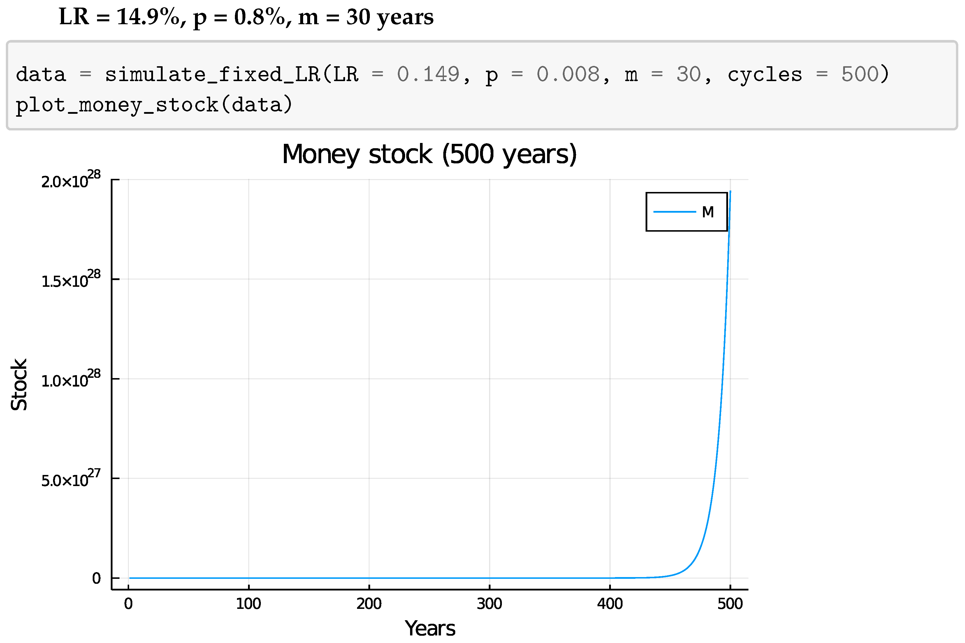
Figure 17. Money stock (LR = 14.9%, p = 0.8%, m = 30 years).
Jrfm 14 00335 g017
Figure 18. Growth ratio (LR = 14.9%, p = 0.8%, m = 30 years).
Jrfm 14 00335 g018
Figure 19. Debt ratio (LR = 14.9%, p = 0.8%, m = 30 years).
Jrfm 14 00335 g019
Figure 20. Debt ratio (g = 5%, p = 1%, m = 20 years).
Jrfm 14 00335 g020
Figure 21. Debt ratio (g = 5%, p = 1%, m = 40 years).
Jrfm 14 00335 g021
Figure 22. Debt ratio (2% <= g <= 12%, p = g - 5%).
Jrfm 14 00335 g022
Figure 23. Debt ratio (2% <= g <= 12%, p = g).
Jrfm 14 00335 g023
Figure 24. Debt ratio (2% <= g <= 12%, p = g + 5%).
Jrfm 14 00335 g024
Figure 25. Debt ratio (g = 4.75%, p = 0.8%).
Jrfm 14 00335 g025
Publisher’s Note: MDPI stays neutral with regard to jurisdictional claims in published maps and institutional affiliations.