
What Can District Migration Rates Tell Us about London’s Functional Urban Area?

Department of Accountancy Finance and Economics, University of Lincoln, Lincoln LN6 7TS, UK
J. Risk Financial Manag. 2023, 16(2), 89; https://doi.org/10.3390/jrfm16020089
Submission received: 18 November 2022
/
Revised: 29 January 2023
/
Accepted: 31 January 2023
/
Published: 2 February 2023
(This article belongs to the Special Issue Shocks, Public Policies and Housing Markets)
Abstract
:In the early 1990s, Anthony Fielding coined the term ‘escalator region’ to describe how London and the South East attracted those with greater human capital by offering them superior career prospects and enhanced returns in the housing markets. When delineating a housing or labour market area, it is not uncommon to require high levels of migration and commuting within the market area relative to those that cross the area’s boundaries. Net migration flows to and from this escalator region change depending on the age range one examines, making migration across boundaries relatively high. It is proposed that focusing on age ranges that reflect younger adults would capture the extent of the market. In particular, the birth of a first child is likely to trigger migration, but that movement is constrained to be within the boundary of the market area. The decision to buy a dwelling would be made around the time of this event. This paper delineates market areas using spatial autocorrelation. This has the advantage of using a statistical criterion rather than a containment value. Broadly similar areas in the Greater South East are revealed using relative housing affordability measures, the movement of infants and the migration of 20- to 24-year-olds. It is argued that the time-varying patterns of migration of 30- to 39-year-olds is reflective of a change in housing affordability, forcing more households to migrate with children whilst renting.
Keywords:
escalator region; local indicators of spatial association; house price–earnings ratios; local authority districts; internal migrationJEL Codes:
R12; R23; R311. Introduction
The spatial general equilibrium framework (Roback 1982) projects that agents relocate within and between nodes to maximise their utility. Locational choice (migration) will account for the commuting to work costs and the associated costs of accommodation. DiPasquale and Wheaton (1996) see a housing market area as derived from workers being able to substitute residences without changing jobs, or switching jobs without moving home. A housing market area is the area in which households live and work. The labour and housing market areas are likely to cover similar geographical spaces. All other things being equal, when they are seeking to move, workers will search for alternative accommodation in the housing market area (Royuela and Vargas 2009). Indeed, migration data can provide an alternative to commuting data for building a housing market area when there are, for instance, no commuting data available (Royuela and Vargas 2009).
Dennett and Stillwell (2010) conclude that net migration rates and spatial patterns vary dramatically when age is taken into consideration. Certain events in an individual’s life are likely to occur. Such life events include education completion, labour force entry, union formation, and birth of their first child (Bernard et al. 2016). Each are likely to trigger migration and changes in housing consumption (Eichholtz and Lindenthal 2014; Jones et al. 2010).
Fielding’s (1992) ‘escalator region’ has echoes of a core region of an unbalance growth model. An escalator region attracts those with the highest human capital offering superior career prospects, where short term disincentives are compensated by the anticipation of longer-term rewards. The most obvious escalator in the UK is London. One would anticipate that union formation and first childbirth would trigger migration within the market area of the region, which could be used to outline its limits.
Champion et al. (2014) considered whether the second-tier cities of Birmingham, Manchester, Leeds, Newcastle, Bristol, Sheffield, Liverpool, Nottingham and Leicester provide the same pace of career advancement for their longer-term residents as for their recent immigrants. Compared with the Greater South East area (GSEA), they find that career acceleration in the second-order cities is less likely. The city areas are defined as ‘city-regions’ that combine the city with other districts from which there is significant commuting.
The objective of the paper is to reveal a Greater South East area using net-migration data provided by the Office for National Statistics (ONS). The age bands selected are posited to capture the movements of younger adults within the Greater South East at different stages of their lives. One additional objective is to link this movement with relatively intense competition for suitable dwellings.
This paper explores migration and house price indicators of escalator regions in England and Wales using migration data that are more narrowly focused than those reported by Dennett and Stillwell (2010). The work here analyses district net migration in the 20–39-year-old age bands. These capture the movements of those younger adults that are in the age ranges that are associated with an escalator region. Dennett and Stillwell observe that the movements of those in the range of 30–45 years is reflected in the migration of children. A novel contribution is to track the migration of pre-school children. Being passive in the move, these infants highlight where their parents are choosing to reside. Parents of 0–4-year-olds are likely to be to seeking their first family-sized dwelling. This ties in with a further contribution. Due to the nature of the labour market, there will be relatively intense competition for dwellings that suit first-time buyers, which will be reflected in the price of a property in relation to the income of those of the area.
The method entails tracing the extent of migration within 0–4 age-band using spatial autocorrelation. The results are compared with those generated when considering the movement of those of 30–39 years of age. In addition, the migration of those in the 20–24-year-old age range is posited to capture the geographical extent of an escalator region. The relative intensity of competition for dwellings is assessed by the house price–earnings ratio. It is proposed that the first-time buyer could choose to sacrifice a greater proportion of their income than other buyers because of the perceived long-term benefits of residing in the region. As such, relative affordability measures should also capture the geographical extent of an escalator region.
The paper is structured as follows. Section 2 provides contextual information about housing and migration. Then, there is a discussion of spatial housing market delineation and a classic monocentric urban model in Section 3. Section 4 entails a review of migration by age group with a focus on graduate movements and a conveyor belt of migrants to and from the London area. The next section concerns the statistical method of delineating markets. The data for house price–earnings ratios, transactions, median age and internal migration are sourced from the Office for National Statistics. It is found that most, but not all, of the migration and affordability indicators reveal a Greater South East area, and that infants have similar migrational patterns to those in their 30s. However, as first-time buyers delay making their purchase, there appears to be a greater tendency for households that rent to migrate as a family unit.
2. Contextual Information
In 2018, there were approximately 34 residential dwelling sales per 1000 dwellings in England and Wales. In London, the rate was 7% lower than any other region at 24. In England and Wales, the purchases of semi-detached, detached and terraced dwellings each comprised 28% of the market, approximately. In London, over half of sales were of flats. Renting is more prevalent in London than in the rest of England, with 28% of households in the Capital in the private rented sector, above the 19% in the rest of England (English Housing Survey 2019).
The English Housing Survey (2019) reveals that the percentage of 25–34-year-olds that owned with a mortgage was around 40% in 2011/12 in England, as was the percentage that privately rented. By 2017/18, the former had decreased by 6%, and the latter increased by 6%. Decreasing affordability is affecting the timing of the change in tenure, as highlighted by the increased age of the first purchase by an additional 1.9 years over 2012–2018 (English Housing Survey 2019).
Around half of those shifting from the private renter sector to owning a dwelling did so within the 25–34 age-band; 83% of those changing tenure were couples, of which 40% had dependent children. This group, the English Household Survey suggests, move into home ownership in order to buy a larger home, perhaps to accommodate a growing family, and leave the private rented sector. Cosh and Gleeson (2020) observe that during 2012–2018, the proportion of those households with children buying with a mortgage (from 44% to 49%) and privately renting (from 33% to 34%) in London increased. The latter rate was 20% in 2004, pointing to a notable change in London’s households that rent.
In 2018, there were just over 3 million persons that migrated across a regional border in England and Wales. With a population of 59 million people, 5% of the population engaged in ‘internal migration’. The largest age band for that was the 15- to 19-year-olds followed by 20- to 24-year-olds, corresponding with participating in and completing higher education and securing the first job. London as a whole had an overall net outflow of people to other areas of England and Wales. London is by far the biggest draw for both young age bands. However, from then on, London has experienced net outward migration. The ONS aligns with Dennett and Stillwell (2010) in reporting a strong age bias in migration both in and out of the London and South East areas. The Office for National Statistics asserts that these moves correspond with families with children tending to leave London, whereas young adults aged in their 20s tend to move to London.
In the UK, the median age for the first-time husband is 31.8 years, with his wife, 1.7 years younger. The average age of first-time mothers is 28.8 years in 2017, with the second time being 2.2 years later. The average age of a birthmother is 30.5, whereas the average age of a father is 2.9 years older.
3. Market Areas and Migration
The travel-to-work area (TTWA) is drawn up to define a local labour market area, based on commuting patterns (Royuela and Vargas 2009). Brown and Hincks (2008) posited that a TTWA is similar to a housing market area. Declaring migration to be the defining feature of a housing market area, the distance someone is willing to relocate whist commuting to the same workplace, is a key measure of the extent of the area. It is defined by a high degree of intra-area migration or commuting, relative to cross-border movements. The ‘high degree’ hinges on a threshold market ‘containment’ parameter, for which there is no ‘natural’ value (Jones et al. 2012).
A functional urban area consists of a densely inhabited city and of a surrounding area (commuting zone) whose labour market is highly integrated with the city (Dijkstra et al. 2019). A functional urban area or a Primary Urban Area (Champion et al. 2014) would correspond with a housing market area in a broad sense. As such, commuting and migration would set the spatial limits.
Spatial autocorrelation offers a statistical approach for delineating a market area, avoiding the need to set a containment value. Aguiara et al. (2020) analysed the total numbers of people making cross-border commuting trips. Rather than examining flows directly, they distinguish Functional Urban Regions from São Paulo state as municipalities with relatively high population zones sat adjacent to high outward-commuting districts. Local indicators of spatial association (LISAs) have been used to reveal housing market areas (Gray 2012; Tu et al. 2007). Tu et al. (2007) revealed that submarkets need not be clustered together geographically: a useful property where dislocated zones are viewed as potential substitute housing areas.
Jones et al. (2012) noted that an additional approach to delineating a housing market area is to use house price levels and/or rates of change. DiPasquale and Wheaton (1996) argue that short-term changes in relative prices that constitute a mispricing of a dwelling should be eroded quickly by switching house-search behaviour within the housing market area, thereby maintaining a structure of prices. The search for housing, the precursor to migration, is a key driver of stable differentials.
It is posited that an area’s attraction to a renter or buyer reflects the characteristics and constraints of their cohort at a point in the life-course. A monocentric urban model posits that there is an employment centre surrounded by dwellings that vary in use of land and price. As commuting is a bad, dwellings closer to the centre are more expensive to rent or buy, ceteris paribus. City-centre or inner area living, usually in high-density dwellings such as flats, for, say, childless households in their 20s and 30s, are traded for outer-area living with the use of a garden at later stages by households with children (Jones et al. 2010; McCann 2013).
Moving to a nearby rural area but retaining the same job or “back commuting” has been typified by Brown et al. (2015) as a conveyor belt. English labour markets are characterised by a significant amount of long-distance commuting. They argue that the rural-urban interface can be understood as an extensive geographic space where particularly higher-status migrants leave a high-density urban environment to live in low-density rural enclave, with an extensive commuting distance to the workplace. This is consistent with the definition of a functional urban area.
Using commuting data and a multi-level modularity optimisation algorithm, Shen and Batty (2019) delineated functional urban areas of eight occupational groups within Metropolitan London. They find that the core routes of the transport network play a part in the locational patterns of the derived communities for each occupation. The number of detected areas is smaller for the populations with more professional- or managerial-oriented occupations than that for the workers in the less-professional groups. Managerial occupations travel longer distances than the other groups, thus making their perceived functional areas larger than those perceived by other occupations of workers who are more diffused across the London Metropolitan region.
Life events affect the decision to migrate. Clark (2013) found that having a child and being married decreases the probability of moving, but the events of marriage and the birth of a child increase the probability of moving. Having a child is negatively related to distance, but being married has a positive relationship with the distance of a move. The birth of a child depresses the likelihood of making an inter-metropolitan move. This reflects staying within one labour market.
Bullen (2015) found that three quarters of the net outflow of the 30–39-year-olds from Manchester in 2013 were to its neighbouring districts of Trafford and Stockport. Moreover, 69% of the net outflow of those aged 0 to 4 years followed this pattern, strongly suggesting that families with pre-school children leave the city centre. These are three of the ten districts in the Greater Manchester functional urban area. Consistent with this, year-on-year, the Office for National Statistics shows that internal migration generally occurs between neighbouring districts, and around half of moves are to areas within the same region.
Using renters as the control group, Lin et al. (2016) found that Taiwanese households that own their own home have their first child at an older age, but have a greater number of children over the fertility cycle. Families living with their parents or siblings become parents at a younger age and also have more children at the end of the fertility cycle, implying that the decision to buy a dwelling is linked to other life constraints. Öst (2012) found a simultaneity between becoming a homeowner and the birth of the first child in Sweden. Affuso et al. (2022) showed that unidirectional causality exists between house prices and fertility. There is a wealth effect in the U.S., so that when house prices increase, this induces families to have more children.
4. Superior Human Capital and Locational Choice
Cumulative causation models in a national economy project unbalance regional growth. Due to enhanced wages, through migration, the advantaged region denudes other provinces of superior human capital. Perpetuating an inequality of performance, advantageous productivity growth boosts pecuniary reward, forming the basis for further immigration to this core region. Migration models complement this view. Those with superior human capital have a greater incentive to search over a wider terrain (McCann 2013). A related concept is Fielding’s (1992, pp. 3–4) escalator region which has implications for this study. The region would attract many young people at the start of their working lives. Subsequently, it would provide the context within which residents achieve accelerated upward social mobility through movement within the region’s labour and housing markets. Towards the end of their working lives, a significant proportion of those who had experienced this upward social mobility leave the region.
Fielding’s (1992) analysis focuses on the young, highly educated graduate migrant and the role of London, but can be applied to other migrants and other cities (Champion et al. 2014). Evidence of a core-escalator region and life-course migration decisions can be found in Kooiman et al.’s (2018) work. They find that between the ages of 16 and 35, Dutch university graduates exhibit spatial trajectories which differ from those who are less-educated. This process occurs in two steps. From the ages of 17 to 22, students relocate to university cities. However, big cities and The Hague continue to be recipients of human capital during the second peak in spatial mobility, which is associated with job search of recent graduates in their mid-twenties, whereas smaller university cities start losing human capital. From age 26 onwards, the share of university graduates in peripheral municipalities is, on average, 40% lower than the national share.
Bernard et al. (2016) found that long distance moves, particularly those that cross regional borders, are strongly associated with both education and labour market entry. Thomas et al. (2019) found that education is the most-cited reason for moves of more than 90 km across the UK, and is the most cited reason in Sweden for moves of more than 80 km. The UK graduate jobs agency, Prospects (2019), charts the first employment destinations of graduates. It describes the university graduate market as ‘urbanised,’ based around London and its environs, and the larger regional centres of the UK. Overall, the degree graduate’s first destination job is dominated by London and the South East, which absorb over a third of the UK crop. Of the fifth of graduates that moved to regions where they were neither domiciled nor studied, 43% ended up in London. In other words, British universities are not exclusively located in nodes at the top of the city-size hierarchy but, consistent with Kooiman et al. (2018), there is further movement following graduation up the hierarchy for some of the most well-qualified individuals.
Levantesi and Piscopo (2020) used a Big Data algorithm to analyse London real estate price data. They find that the effects of the population, annual growth in households with a mortgage and net housing supply are the key variables that capture the interaction between housing demand supply and price. Constrained dwelling supply and a rising population point to increasing London prices and rents. Although they do not consider income, their work points to declining affordability in the Capital. Gray (2022) shows that a key measure of affordability, the house price–earnings ratio, in the South East of England continued to grow long after the financial crisis of 2008, which is at odds with the rest of Britain. He argues that this decreasing affordability is, in part, based on expected future growth rates. Anticipated income growth generates higher local house prices for a given income level in the escalator region. Mortgage lenders will see those with greater human capital as lower risk-borrowers, with a corresponding favourable disposition to repay greater debt.
Again, comparing the motives to migrate in Sweden and the UK, Thomas et al. (2019) found that housing is the most commonly cited motive when moving distances of less than 20 km. Dennett and Stillwell (2010) trace the patterns of London migrants aged 0–15. They observe a tendency to move to less dense housing. Specifically, they see a move from central London to outer London; from outer London to surrounding Commuter Belt or rural areas; or from Commuter Belt to rural areas. In accord with this, the Mayor of London’s Office data show that outward migration of the Capital’s 0- to 3-year-olds is concentrated in the East of England and South East regions (70%). In 2018H1, Hamptons (2018) found that 31% of London’s first-time house buyers bought outside London with 85% moving to those two neighbouring regions. More homes were bought by Londoners than existing residents in seven Local Authority Districts. Thus, house purchase of the first-time buyer is posited to be linked to child rearing. Tracing migrants aged 0–4 years old should provide a similar pattern of motion to that which Dennett and Stillwell (2010) suggest; however, by using a narrower age band, it should better focus on the activities of the younger person, who is more likely to be a first-time buyer.
The net outward-migration phase at the end of the link with the escalator region, where a significant proportion of those who had experienced this upward social mobility leave the area, is likely to be related to older households with higher value dwellings taking advantage of their housing equity and the greater freedoms that early retirement might bring. It is expected that his group is dispersed across many regions and likely to relocate to more rural areas (Li et al. 2022).
5. Research Method
The net migration rate in age band a per 10,000 population in area i (NMRia) is defined as where is the net migration rate; Ii is the number of people that are found to have relocated to the area, or inward-migration to area i; Oi is the number of people that have relocated from an area, or outward-migration from that area; and POPi is the population of that area (Dennett and Stillwell 2010). This is similar to the migration efficiency index found in Lomax et al. (2014) but offers a view on whether there is net inward or outward migration.
Rather than using house prices to delineate housing market areas, a perhaps under-utilised indicator is the affordability ratio. A house price–earnings ratio can be measured by dividing house price (HP) by earnings (E). The house price–earnings ratio of district i ratio could be . One of the advantages of such a ratio is that one money variable is divided by another so that time and international comparisons, such as those by Demographica (2022), can be made without due concerns about exchange rates or inflation distortions. Additionally, the spatial general equilibrium framework predicts higher living costs is weighed against higher rewards when choosing a location, implying a house price–earnings-ratio-based indicator might be more appropriate than purely a price one.
The Office for National Statistics provide two categories of house price–earnings ratio. The ratio estimated at the median (M) is interpreted as reflecting affordability for non-first-time buyers. The second, lower quartile (LQ) data have been used by Wilcox and Bramley (2010) as a proxy for housing affordability of first-time buyers. They argue that 40% of all first-time buyers in a year purchase a dwelling at or below the lower quartile prices, whilst on average around 15% of repeat buyers with a mortgage purchased dwellings at or below lower quartile prices.
It is proposed here that as the two ratios reflect distinct market segments, the spread between them can highlight locational preferences and market conditions. The spread, or the district house price earnings ratio differential (HPERD), is defined as . For the sake of framing the ideas and language, assume each district has the same distribution of buyers and dwelling types and that so in a standard territory both buyer-groups face the same house price–earnings ratio, and HPERDi = 0. A standard wage compensation hypothesis would project that a territory with enhanced amenities should experience a lower relative wage (and higher house price) at both the median and lower quartile, suggesting HPERi > HPERj, where district i has superior amenities. This would include proximity to job opportunities. Assuming larger properties are favoured by older buyers, or there is a preponderance of higher income buyers, competition for larger units should drive up these dwelling prices, results in a positive spread value. Simply put . Constrained to look for smaller dwellings, a preponderance of modest earners in district i could lower average earnings whilst intensifying competition for such dwellings, leading to affordability at the lower quartile to be more challenging that at the median, or a negative spread value.
Moran’s I, a global measure of spatial association, involves correlating a variable with the spatial weighted average of itself, so that it can provide an indication of (dis)similar values across space. Local indicators of spatial association (LISA) make up the components. A LISA is defined as (Anselin 1995) where . The extent of a revealed cluster depends on the type of weight matrix and the limits associated with it. A distance matrix is selected as it can capture association between non-contiguous spaces. A distance limit of 80 km or 50 miles reflects a one-hour journey to London on the fastest trains from such places as Bedford and Brighten (north and south of London) or Colchester in the East of England, plus the university centres of Oxford and Cambridge. The (inverse) distance between areas i and j are used for the elements of the distance weights matrix, wij = and wii = 0, so that those spaces that are closer together have a greater weight. To cater for multiple statistical comparisons, the level of significance is adjusted. Anselin (1995) argues a Bonferroni adjustment is too conservative. Le Gallo and Ertur (2003) recommend the adjustment be based on the number of near neighbours. All bar five districts have 10 or fewer neighbours, so the adjustment entails using 0.5% pseudo-level of significance, which corresponds with a false discovery rate of around 0.25%.
As an example, local indicators of the spatial association among 0–4-year-old migrants are interpreted. Under the null that the distribution of net migration rates (NMRs) across the districts of England and Wales is random, it suggests that localised differences are not distinctive. A low–low (LL) combination reflects co-located districts with statistically significant net outward migration rates of 0–4-year-olds, signifying that their parents are leaving these districts. In a monocentric urban model, complementarity in net inward migration should reveal an outer ring of high–low (HL) districts, indicative of their parents relocating there. High–high clusters are those with districts than have high rates of net inward-migration of youngsters. They could be adjacent to low–high districts, which experience net outward migration. The movement of youngsters should be reflected in adult migration patterns and housing affordability differences.
6. Data
Excluding the Isles of Scilly which have intermittent data, there are values for 338 English and Welsh Local Authority Districts on migration, house price and earnings, supplied by the Office for National Statistics (ONS 2020). Each year, the ONS receives a demographic snapshot of Patient Register data held by NHS Digital. Internal migration for Local Authorities in England and Wales, by five-year age groups, year ending June 2012 and 2018 are used for both districts and regions. Internal migration estimates are weighted by the mid-year population estimate for the territory.
The Office for National Statistics generates affordability indices (ONS 2020) by dividing the district house price by the district earnings at both median and lower quartile levels. House Price Statistics for Small Areas are drawn from the Land Registry, which provides a comprehensive record of property transactions in the UK. Nomis provides the median population age for each district. Earnings data are taken from the Annual Survey of Hours and Earnings. Annual estimates of gross earnings are based on the reference tax year and relate to employees on adult rates of pay who have been in the same job for more than a year. Both workplace-based and residential district earnings are available. Work-based data are used to reflect the likely commuting of workers across district borders, a key feature of a functional urban area.
7. Results
From Figure 1a, one can discern the age distribution of residents across space for 2018. A quantile map for four groups, ranked by age, shows that the ‘youngest 84′ districts by average age (in black) are quite often city ‘pinpricks’. Larger centres include London and Leeds. This strongly reflects the view that cities attract the young. The grey patches capture towns and their hinterlands. The yellow reflects the ‘oldest’ areas. It is interesting to observe that there is no clear gradation of black through to yellow arranged in some concentric circles. Rather, city black is adjacent to rural brown or yellow. The exception, though, is London.
Figure 1b displays a map of local indicators of spatial association for the same data. The outstanding feature is that a Greater South East area emerges comprising blue LL areas separating two pink HL districts. This area is much larger than Greater London’s 33 boroughs. There are concentrations of older folk in the Devon area and Wales. However, statistically, only London shows a concentration one would expect from an escalator region. The Greater South East area strongly aligns with the limits presented by Shen and Batty (2019).
7.1. Concentrations of Districts That Attract the First Time Buyer
Figure 2a,b display maps of local indicators of spatial associations among spreads (or HPERDs) for 2012 and 2018. The outstanding feature is that a greater South East area emerges comprising blue LL areas interspersed with pink HL districts in both figures. There are 110 highlighted districts in 2018. The 89 LL districts contain relatively expensive houses at the lower quartile, which are posited to be reflecting the purchases of the first-time buyer. The other 31 are districts that have high house price–earnings ratios at the median relative to the local lower quartile ones. These are more rural in nature. Greater London itself is not entirely blue. The method reveals very expensive west end suburbs including Kensington and Chelsea. The inference here is that an area classified as severely unaffordable (Demographica 2022) is particularly expensive for the first-time buyer.
HH combinations suggest the north of England contains adjacent districts where the house price–earnings ratio differential is greater than in other regions. A light blue patch captures a district that is relatively expensive at the lower quartile, locally. An example is the rural district of Ribble Valley, a LH-classified district that has a house price–earnings ratio at the lower quartile of 7.83 in 2018. Preston, a city and its neighbour, has a house price–earnings ratio of 4.32 and a positive differential. Housing in Ribble Valley is 55% more costly than in Preston, but (workplace) earnings are lower. The attraction of rurality combined with commuting is consistent with Bullen’s (2015) and Bernard et al.’s (2016) work. This HH–LH combination comprises Manchester, Leeds, Sheffield and Preston, a polycentric ‘Northern Powerhouse’. London emerges as an area where the urban spreads are commonly negative, whilst the Northern Powerhouse appears as the obverse.
Figure 2c displays a quartile map of the number of sales of detached dwellings divided by the sales of terraced properties in 2018. As urban areas would feature a more intense use of land, a low ratio should highlight cities. Again, the colour black highlights urban areas. The band from Wales to the east coast of the East Midlands coloured yellow shows where detached dwellings are sold in relatively high proportions. These areas are more likely to be rural and house an older age group. An extended London, coloured grey or black, echoes the findings shown in Figure 1a, suggesting that younger people occupy spaces where there is a relatively high rate of terraced dwellings sold.
7.2. Migrational Spatial Associations
Table 1 displays the regional net migration data for 2018, weighted by population, covering 5-year intervals of working age. The table reports inter-regional migration for those aged 20 to 64 years old. A key observation is that the net-migration in the first age-band is, for most regions, in the opposite direction to the third. The first band, the one with the greatest degree of net migration, combines job securing as well as returning home from higher education. Both are more likely to entail long distance migration. The post-50 age group tends to leave the Greater South East area and migrate elsewhere.
The age-bands highlight why, as a measure of containment, net migration can be problematic. With a threshold value of 1.5 one could say that many regions are ‘contained’ units. The North West and South East have low net (mean) migration rates but the variation over the age-band, as measured by standard deviation, is very different. The former has the lowest standard deviation, whereas the latter, posited to be integrated into the Greater South East area, has a high-level of cross-border migration. Wales and the South West appear not dissimilar in the later age-bands, subject to net inward migration. The North East and Yorkshire–Humberside, traditionally poorer regions, lose their youth as Wales and the South West do, but they are not replaced in the early retirement period.
For the UK’s regional system, the long-distance migration is focused on London for 20–24-year-olds. The peak post-university net change is in the 30–39-year-bands, out of London. This exit appears to be accommodated in the southern regions with a high rate of net inward-migration, echoing the Mayor of London Office’s data on infants.
Figure 3 displays local indicators of spatial association of migrants for two age-bands (0–4 and 20–24) for 2012 and 2018. As anticipated, there is a clear pattern of inward-migration to London in the 20–24 band. Figure 3c,d support the view that there is no alternative attractor centre away from London. The blue patches include Luton, Cambridge, Reading and Brighton, which would lose migrants as students leave university. The extensive commuting networks around London allows for integrated rural areas to form part of an extended functional urban area. The extent of the Greater South East Area appears stable across the two years. There are strong commonalities between Figure 1b, Figure 2b and Figure 3d in this extended London area.
Despite a lower average age and the inflow of younger adults after graduation, the Capital has a low fertility rate (ONS 2019). Figure 3a,b map local indicators of spatial association of migrant infants in 2012 and 2018. Blue LL combinations, more evident in 2018, contain adjacent districts where the net flow of very young children is negative. This area includes inner and some outer London districts. The pink HL combinations feature a net inflow. There are obvious concentric rings. In the light of other work (Dennett and Stillwell 2010; Mayor of London; Hamptons 2018), the interpretation is that net outward-migration in this age bracket is dominated by migration from London to the South East and the East of England. Importantly, this is within an 80 km radius of central London outlined above as proxy for a commutable distance by rail. The Greater South East area emerges again.
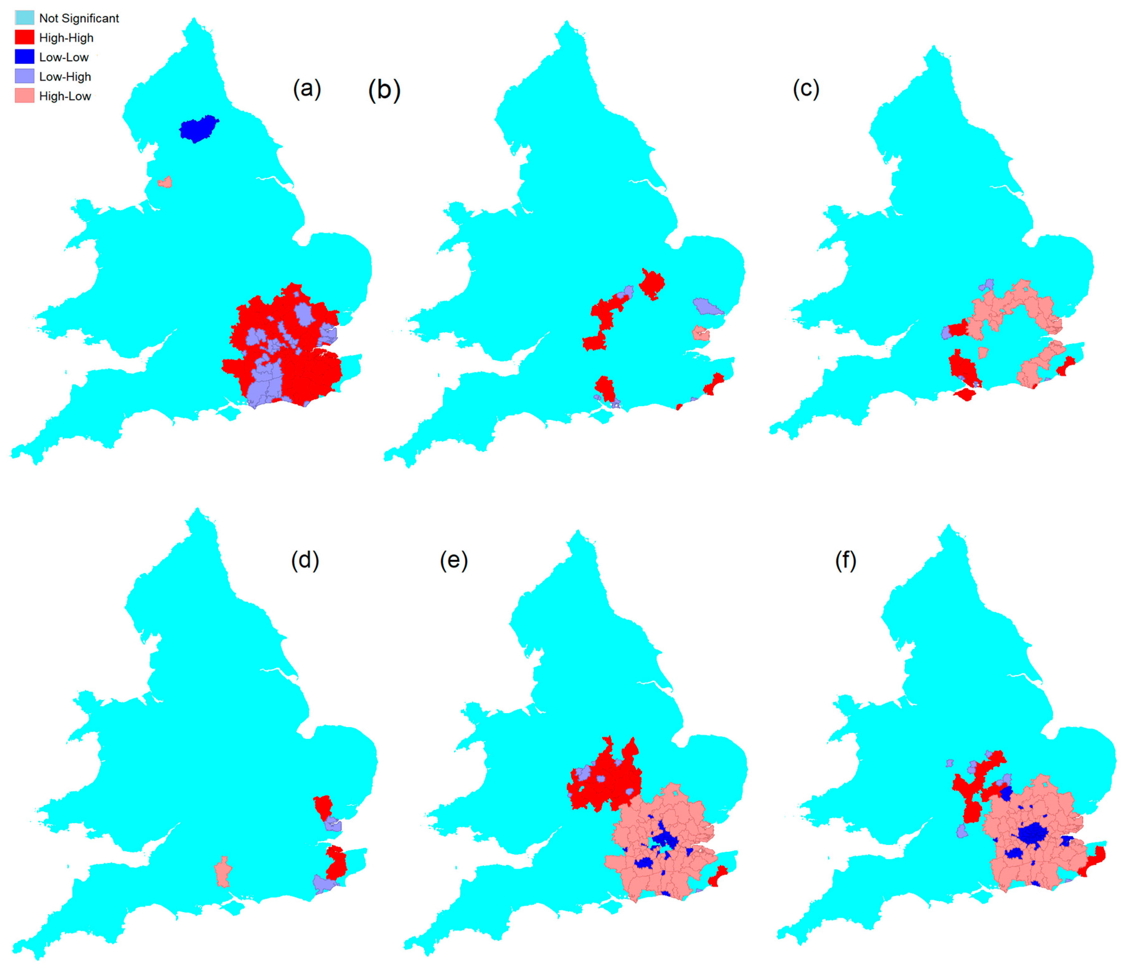
Figure 4 covers three more age-bands (25 to 39) posited to be associated with union, dwelling purchase and first child. For 2012 (Figure 4a–c), there appears to be transition from net inward- to outward-migration. The pattern with 25–29-year-olds (Figure 4a) points to young adults moving into the Greater South East area from outside London in search of employment. The extent of the coloured area relates those of 20–24- and 0–4-year-olds. The extent of the zone in Figure 4c, associated with 35–39-year-olds, resembles that of Figure 4a. Dennett and Stillwell (2010) make the point that the migration patterns of 0–15-year-olds are similar to those of 30–45-year-olds. By tracking migration patterns of children one can gauge the migration of their parents. Rather than a broad 15-year age band, there is a focus on 0–4-year-olds. From this, it is inferred that the spaces traced reflect parents leaving Greater London to relocate to less densely populated districts with their young children.
The disjointed nature does not preclude the territories being viewed as part of the same housing market (Tu et al. 2007). The pattern for Figure 4b is of a ring with a larger radius than the other ones mentioned. Including places such as Hastings on the south coast and Northampton in the east midlands, the distance to London is around 100 km is, perhaps, too far to back-commute for all but the hardiest commuter. The void inside perhaps reflects job-seeking interlopers matched by the outward migration of those looking for less densely populated districts or as Dennett and Stillwell (2010) suggest, those from outer London moving beyond the border to be replaced by those from inner London.
The corresponding diagrams for 2018 could reveal a time shift. Figure 4d for 25–29-year-olds is similar to Figure 4b whereas Figure 4e,f, covering 30–39-year-olds, are very similar to the Greater South East area in Figure 3b. The English Housing Survey (2019) revealed that the percentage of 25–34-year-olds that owned with a mortgage or privately rented in 2011/12 in England was around 40%. By 2017/18, the former had decreased by 6%, and the latter increased by 6%. Decreasing affordability affects the timing of the purchase as highlighted by the increased age at the first purchase, by an additional 1.9 years over 2012–2018. Renting is more prevalent in London than in the rest of England, with 28% of households in the Capital in the private rented sector, above the 19% in the rest of England. Cosh and Gleeson (2020) observe that during 2012–2018, the proportion of those households with children buying with a mortgage (from 44% to 49%) and privately renting (from 33% to 34%) in London increased. The child-rearing phase, when either owning or renting, is likely be linked to migration to lower dwelling density areas. It could be that Figure 4e,f maps reflect back-commuting of buyers and, increasingly, renters in the same districts looking for greater dwelling space for their children.
The red HH spots in Figure 4e,f are concentrated in the midlands. They also have an echo in Figure 3b. The associated blue patches reflect cities. There is short distance migration from inside the urban centres to neighbouring districts outside. The West Midlands has a relatively high fertility rate.
Using the LISA results for 0–4-year-olds (so corresponding with Figure 3b) as the basis of analysis, Table 2 reports that there are 186 districts classified as not significant; 52 are classified as in LL clusters; and 55 classified as the adjacent HL combinations. With 11 million residents, the LL districts have a greater population than the 33 boroughs of London (8.9 million). The net outward-migration of 0–4-year-olds numbers 20,000, generating the migration rate of –18.04, which not dissimilar from the value seen in Table 1 for London’s 30–34-year-olds. The HL combinations nearby absorb 8000 youngsters. The HH districts receive a greater influx of youngsters than the complementing LH districts donate, which reflects some migrants moving directly into those areas from elsewhere. For both LL–HL and LH–HH combinations, there are corresponding population density swings, which is indicative of the desire for greater space. Plus, there is a 5-to-6-year average age gap between the donor and the recipient districts. The LL–HL area is taken to reveal a Greater South East area, whilst the LH-HH zone highlights a midlands polycentric area.
Using the LISA results for affordability differential (so corresponding with Figure 2b) as the basis of analysis, the LL–HL combinations have a population of over 20 million. Both areas have a net outward migration of youngsters. The average affordability ratios for LL and HL districts are about the same at the lower quartile but differ at the median, indicative of a positive differential for lower density districts.
7.3. Coincidence of Cluster Types—Revealed Region
The LL–HL combination of both the spread and youngster LISA maps appear to capture a Greater South East area seen in movements of 20–24-year-olds. Of the 107, LL–HL combinations highlighted using the infant migration data for 2018, 101 correspond with the spread-based LL–HL districts (of which there are 120). In Table 2(c), the overlap is analysed, so that the Greater South East area is split into a 2 × 2 grid. Of the LL–LL combinations, 23 are in Greater London. Those outside London include urban centres in the East of England (Cambridge, Stevenage and Broxbourne).
The LL–LH combinations in Table 2(b) have similar price-earnings ratios and average ages indicating the house price–earnings ratios have revealed a common market. The subdivision in Table 2(c) into LL(infants)–HL(spreads) and LL–LL does not reveal much. They have the same mean age and net outward-migration rate of youngsters. The combinations of recipient districts have a higher mean age and lower density living. The LL–LL combination districts are less affordable at the lower quartile consistent with expectations, whereas LL–HL have the obverse. It is concluded that the pattern of child movement is not necessarily related to affordability spreads.
8. Discussion
Fielding (1992) asserts that there are both housing and career benefits that attract young adults into an escalator region. He is not specific about internal migration post education completion and labour force entry but anticipates movement within these markets. It is suggested that life events, such as union formation and the first child, are likely to trigger migration and greater housing consumption. As the escalator region should lose its older population, net migration across all ages is not appropriate for delineating this type of functional urban area. Narrow age bands associated with the younger adult better fit Fielding’s vision.
The extent of the Greater South East area is traced out by two different groups: those attracted in, looking for a good start to their career; and those possibly moving with their children. Net inward-migration of those aged (20–24 years) point to initial attractor stage of an escalator. The net outward-migration from London of those aged 0–4 demarks the same space but in the form of concentric zones. Infant migration possibly from inner to outer South East is consistent with Dennett and Stillwell (2010). These infants would migrate with their parents. Indeed, the movements of the 30–39-year-olds mirror the migration patterns of infants. Those in that attractor stage are unlikely to be looking for the same type of dwelling as the parents. A uniting factor is likely to be the transport infrastructure that would strongly influence the process of back-commuting.
It is asserted that competition for dwellings suitable for the younger buyer will drive up the house price–earnings ratio for that group. There is evidence that the decision to have children is related to house purchase (Öst 2012) so the migration of younger people should herald where there will be competition for the smaller dwelling suitable for child-rearing. The areas where the intensity of competition for such a dwelling as revealed by house price earnings ratios are in line with the extent of the movements of younger adults and infants.
Comparing the mapping with the Nationwide Building Society’s delineation of regions, whose data are used by the British government when reporting house price movements, the Greater South East area traces a very similar boundary to that of the Outer Metropolitan area. We included 2 districts from East Anglia and 17 from the Outer South East. Additionally, it is similar to Shen and Batty’s (2019) London Metropolitan area.
Three points are made about the peculiarities of London. First, the movement out of London to surrounding, commutable areas where population density is lower, is likely to be more pronounced because of London’s unusual dwelling portfolio, which uses land intensively and is less suited for children; because migration is more likely to reflect those with superior capabilities; and because of the superior transport network that allows more extensive back-commuting than other UK cities. Champion et al.’s (2014) alternative escalator regions are not as obvious as they could be. Perhaps candidate cities in the north of England, such as Greater Manchester, do not have the same housing structure or affordability constraints, so that the extent of migration at key stages in life is possibly suppressed.
Second, the migration featured has been linked to childbirth and house purchase (Öst 2012). There is a rise in the number of renting family households that are migrating (Cosh and Gleeson 2020). The movements of the 30–39-year-olds indicated in Figure 4e,f closely mirror the migration patterns of infants. There appears to be an earlier rather than a later move from London in 2018 compared with 2012, despite a rapid increase in the average age of the first-time buyer in London. It is posited that the rising costs of housing, causing increasing numbers of buyers to migrate and back-commute, is being emulated by a notable growth in families with children migrating whilst renting. This could be linked to another factor excluding younger Londoners from home ownership. Coates et al. (2015) and Pryce and Sprigings (2009) examined the rise of the absentee landlord (buy-to-let). They find that buy-to-let purchasers compete in the same segment of the housing market as first-time buyers, displacing them, keeping them in the rented sector for longer. Movements of infants would increasingly reflect parents that are renters, suggesting the events of childbirth and first purchase (Öst 2012) is not as strongly associated in the Greater South East Area as they once were. It could be that the escalator region’s housing benefits are for a decreasing minority.
Third, London is also the most common region of first residence for international migrants to the UK. Once established, when some of these move later to other regions, potentially also with children, they would be classified as internal migrants, inflating the net outward migration rate.
9. Conclusions
An ‘escalator region’ is posited to attract those with the high human capital offering superior career prospects and housing benefits. There is movement around the region during the much of their working life, but there is a tendency to leave it towards the end (Fielding 1992).
Migration is used a delineator of a housing or labour market area. Net migration flows change direction depending on the age of the migrant, implying that if broad age-bands are employed to delineate an escalator region, it might obscure important movements of people. Rather than a migration of those of all ages of work, a novel approach to market area delineation entails focusing on narrow age bands that reflect migration triggers of those of younger working ages. It is shown that multiple narrow age-bands reflect that there are large net migrational flows, as predicted by Fielding’s thesis. The first age-group of note, those aged 20–24 years, display net inward migration to an extended London, or Greater South East area. Once in the area, there should be some movement around it. Bullen’s (2015) work and the Mayor of London’s Office data on infant migration point to an alternative means of capturing a functional urban area. Tracing the movement of children should provide a useful proxy for the migration of working-age parents, an observation made by Dennett and Stillwell (2010) and the similarity of movement between 0–15-year-olds and those aged 30–44.
As a substitute for a migration containment threshold over all age groups, the approach to revealing the extent of such a region entails using local indicators of spatial association. A variety of concentric circles emerge. Infant net migration to ‘commutable rural’ appears to be consistent over time. The movement of 30–39-year-olds in 2018 aligns with that of the infants. However, migration maps of those in the 25–39 age groups do not paint quite the same picture as they did in 2012, a period of rapidly decreasing housing affordability.
One implication from this work is that previous research about birth choices and tenure may have to be revised. There is evidence that the decision to have children is related to house purchase (Öst 2012) and that the timing of the purchase is being delayed (Lin et al. 2016). A consequence should be to rent for longer. As such, there is an increase in the proportion of family moves whilst renting (Cosh and Gleeson 2020). It could be that the escalator region’s housing benefits are for a decreasing minority.
A policy implication concerns a reconsideration of the buy-to-let buyer and their function in the housing market. It is argued that the buy-to-let market absorbs some of those dwellings the first-time buyer would consider, making the first house purchase less feasible. To reduce the problem of overcrowding, if more are locked into renting, perhaps the institutional buy-to-rent provider should be encouraged to provide housing services for young family units, a market sector upon which such a provider is not focused (BPF 2022).
The paper delineates the extent of an escalator region using two measures. One limitation of this paper is that the approach to revealing such a functional urban area disfavours candidate city-regions in the north of England, such as Greater Manchester. Careers might be accelerated and there may be favourable housing benefits, but these are obscured by the weight of the London effect on flows and prices.
Funding
This research received no external funding.
Institutional Review Board Statement
Not applicable.
Informed Consent Statement
Not applicable.
Data Availability Statement
All data used are publicly available. https://data.london.gov.uk/dataset/internal-migration-flows-school-age-children-visualisation. https://www.ons.gov.uk/peoplepopulationandcommunity/housing/datasets/numberofresidentialpropertysalesfornationalandsubnationalgeographiesquarterlyrollingyearhpssadataset06. https://data.gov.uk/dataset/dc028a39-d407-4e2c-a430-5f4a3c04ee16/local-authority-district-to-urban-audit-core-cities-greater-cities-and-functional-urban-areas-december-2016-lookup-for-the-united-kingdom (accessed on 30 December 2022).
Conflicts of Interest
The authors declare no conflict of interest.
References
- Affuso, Ermanno, Khandokar Istiak, and James Swofford. 2022. Interest Rates, House Prices, Fertility, and the Macroeconomy. Journal of Risk and Financial Management 15: 403. [Google Scholar] [CrossRef]
- Aguiara, Larissa, Gustavo Garcia Manzato, and Antônio Rodrigues da Silva. 2020. Combining travel and population data through a bivariate spatial analysis to define Functional Urban Regions. Journal of Transport Geography 82: 102565. [Google Scholar] [CrossRef]
- Anselin, Luc. 1995. Local Indicators of Spatial Association—LISA. Geographical Analysis 27: 96–115. [Google Scholar] [CrossRef]
- Bernard, Aude, Martin Bell, and Elin Charles-Edwards. 2016. Internal migration age patterns and the transition to adulthood: Australia and Great Britain compared. Journal of Population Research 33: 123–46. [Google Scholar] [CrossRef]
- BPF. 2022. Who Lives in Build to Rent? British Property Federation. Available online: https://bpf.org.uk/our-work/research-and-briefings/ (accessed on 31 December 2022).
- Brown, David, Tony Champion, Mike Coombes, and Colin Wymer. 2015. The Migration-commuting nexus in rural England. A longitudinal analysis. Journal of Rural Studies 41: 118–28. [Google Scholar] [CrossRef]
- Brown, Peter, and Steve Hincks. 2008. A Framework for Housing Market Area Delineation: Principles and Application. Urban Studies 45: 2225–47. [Google Scholar] [CrossRef]
- Bullen, Elisa. 2015. Manchester Migration; Manchester City Council. Available online: https://www.manchester.gov.uk/download/downloads/id/22894/a05_profile_of_migration_in_manchester_2015.pdf (accessed on 20 May 2020).
- Champion, Tony, Mike Coombes, and Ian Gordon. 2014. How Far do England’s Second-Order Cities Emulate London as Human-Capital ‘Escalators’? Population Space & Place 20: 421–33. [Google Scholar]
- Clark, William. 2013. Life Course Events and Residential Change: Unpacking Age Effects on the Probability of Moving. Journal of Population Research 30: 319–34. [Google Scholar] [CrossRef]
- Coates, Dermot, Reamonn Lydon, and Yvonne McCarthy. 2015. House Price Volatility: The Role of Different Buyer Types. Economic Letters No. 02/EL/15. Dublin: Central Bank of Ireland. [Google Scholar]
- Cosh, Georgie, and James Gleeson. 2020. Housing in London 2020: The evidence base for the London Housing Strategy. London: Greater London Authority. [Google Scholar]
- Demographica. 2022. Demographia International Housing Affordability Survey. 2022 Edition. Available online: http://www.demographia.com/dhi.pdf (accessed on 30 December 2022).
- Dennett, Adam, and John Stillwell. 2010. Internal Migration in Britain, 2000–2001, Examined through An Area Classification Framework. Population, Space and Place 16: 517–38. Available online: https://www.oecd.org/cfe/regionaldevelopment/functional-urban-areas.htm (accessed on 1 February 2023). [CrossRef]
- Dijkstra, Lewis, Hugo Poelman, and Paolo Veneri. 2019. The EU-OECD Definition of a Functional Urban Area. OECD Regional Development Working Papers No. 2019/11. Paris: OECD Publishing. Available online: https://doi.org/10.1787/d58cb34d-en (accessed on 30 December 2022).
- DiPasquale, Denise, and William C. Wheaton. 1996. Urban Economics and Real Estate Markets. Englewood Cliffs: Prentice Hall. [Google Scholar]
- Eichholtz, Piet, and Thies Lindenthal. 2014. Demographics, Human Capital and the Demand for Housing. Journal of Housing Economics 26: 19–32. [Google Scholar] [CrossRef]
- English Housing Survey. 2019. English Housing Survey Home Ownership, 2017–2018; Ministry of Housing, Communities and Local Government. Available online: https://assets.publishing.service.gov.uk/government/uploads/system/uploads/attachment_data/file/817623/EHS_2017-18_Home_ownership_report.pdf (accessed on 30 December 2022).
- Fielding, Anthony J. 1992. Migration and social mobility: South east England as an escalator region. Regional Studies 26: 1–15. [Google Scholar] [CrossRef] [PubMed]
- Gray, David. 2012. District House Price Movements in England and Wales 1997-2007: An Exploratory Spatial Data Analysis Approach. Urban Studies 49: 1411–34. [Google Scholar] [CrossRef]
- Gray, David. 2022. How Have District-Based House Price Earnings Ratios Evolved in England and Wales? Journal of Risk and Financial Management 15: 351. [Google Scholar] [CrossRef]
- Hamptons. 2018. Outmigration Rise London Leavers Heading North. Available online: https://www.hamptons.co.uk/research/pr/2018/Outmigration-Rise-London-Leavers-Heading-North-August2018.pdf/ (accessed on 30 December 2022).
- Kooiman, Niels, Jan Latten, and Marco Bontje. 2018. Human Capital Migration: A Longitudinal Perspective. Tijdschrift voor Economische en Sociale Geografie 109: 644–60. [Google Scholar] [CrossRef]
- Jones, Colin, Mike Coombes, and Cecilia Wong. 2010. Geography of Housing Market Areas in England. London: Department for Communities and Local Government. [Google Scholar]
- Jones, Colin, Mike Coombes, Neil Dunse, David Watkins, and Colin Wymer. 2012. Tiered Housing Markets and their Relationship to Labour Market Areas. Urban Studies 49: 2633–50. [Google Scholar] [CrossRef]
- Le Gallo, Julie, and Cem Ertur. 2003. Exploratory Spatial Data Analysis of the Distribution of Regional per Capita GDP in Europe, 1980–1995. Papers in Regional Science 82: 175–201. [Google Scholar] [CrossRef]
- Levantesi, Susanna, and Gabriella Piscopo. 2020. The Importance of Economic Variables on London Real Estate Market: A Random Forest Approach. Risks 8: 112. [Google Scholar] [CrossRef]
- Li, Rita Yi Man, Miao Shi, Derek Asante Abankwa, Yishuang Xu, Amy Richter, Kelvin Tsun Wai Ng, and Lingxi Song. 2022. Exploring the Market Requirements for Smart and Traditional Ageing Housing Units: A Mixed Methods Approach. Smart Cities 5: 1752–75. [Google Scholar] [CrossRef]
- Lin, Pei-Syuan, Chin-Oh Chang, and Tien Foo Sing. 2016. Do housing options affect child birth decisions? Evidence from Taiwan Urban Studies 53: 3527–46. [Google Scholar] [CrossRef]
- Lomax, Nik, John Stillwell, Paul Norman, and Phil Rees. 2014. Internal Migration in the United Kingdom: Analysis of an Estimated Inter-District Time Series, 2001–2011. Applied Spatial Analysis and Policy 7: 25–45. [Google Scholar] [CrossRef]
- McCann, Philip. 2013. Modern Urban and Regional Economics, 2nd ed. Oxford: Oxford University Press. [Google Scholar]
- ONS. 2019. Births in England and Wales: 2018 Live Births, Stillbirths and the Intensity of Childbearing, Measured by the Total Fertility Rate. Office for National Statistics. Available online: https://www.ons.gov.uk/peoplepopulationandcommunity/birthsdeathsandmarriages/livebirths/bulletins/birthsummarytablesenglandandwales/2018 (accessed on 30 December 2022).
- ONS. 2020. Research Output: Alternative Measures of Housing Affordability, Financial Year Ending 2018. Office for National Statistics. Available online: https://www.ons.gov.uk/peoplepopulationandcommunity/housing/articles/alternativemeasuresofhousingaffordability/financialyearending2018 (accessed on 30 December 2022).
- Öst, Cecilia Enström. 2012. Housing and Children: Simultaneous Decisions?—A Cohort Study of Young Adults’ Housing and Family Formation Decision. Journal of Population Economics 25: 349–66. [Google Scholar]
- Prospects. 2019. What Do Graduates Do? Regional Edition 2019/20. Manchester: Graduate Prospects Ltd. Available online: https://luminate.prospects.ac.uk/what-do-graduates-do-regional-edition (accessed on 1 February 2023).
- Pryce, Gwilym, and Nigel Sprigings. 2009. Outlook for UK Housing and the Implications for Policy: Are we Reaping what we have Sown? International Journal of Housing Markets and Analysis 2: 145–66. [Google Scholar] [CrossRef]
- Roback, Jennifer. 1982. Wages, rents, and the quality of life. Journal of Political Economy 90: 1257–78. [Google Scholar] [CrossRef]
- Royuela, Vicente, and Miguel Vargas. 2009. Defining Housing Market Areas Using Commuting and Migration Algorithms: Catalonia (Spain) as a Case Study. Urban Studies 46: 2381–98. [Google Scholar] [CrossRef]
- Shen, Yao, and Michael Batty. 2019. Delineating the perceived functional regions of London from commuting flows. Environment and Planning A: Economy and Space 51: 547–50. [Google Scholar] [CrossRef]
- Thomas, Michael, Brian Gillespie, and Nik Lomax. 2019. Variations in Migration Motives over Distance. Demographic Research 40: 1097–109. [Google Scholar] [CrossRef] [Green Version]
- Tu, Yong, Hua Sun, and Shi-Ming Yu. 2007. Spatial Autocorrelations and Urban Housing Market Segmentation. Journal of Real Estate Finance & Economics 34: 385–406. [Google Scholar]
- Wilcox, Steve, and Glen Bramley. 2010. Evaluating Requirements for Market and Affordable Housing; York: National Housing and Planning Advice Unit. Available online: www.communities.gov.uk/nhpau (accessed on 13 April 2020).
Figure 1.
Age Distribution. (a) is a map displaying age by quantiles. (b) is a map of local indicators of the spatial association of the same data.
Figure 1.
Age Distribution. (a) is a map displaying age by quantiles. (b) is a map of local indicators of the spatial association of the same data.

Figure 2.
LISA Housing Maps. (a,b) are maps of local indicators of spatial association of house price–earnings ratio differentials. (c) is a quantile map of the number of sales of detached dwellings divided by the sales of terraced properties.
Figure 2.
LISA Housing Maps. (a,b) are maps of local indicators of spatial association of house price–earnings ratio differentials. (c) is a quantile map of the number of sales of detached dwellings divided by the sales of terraced properties.

Figure 3.
LISA Maps Migration (0–4 and 20–24 years old). (a) Range of 0–4-year-olds in 2012; (b) 0–4 year olds in 2018; (c) 20–24 year olds in 2012; (d) 20–24 year olds in 2018.
Figure 3.
LISA Maps Migration (0–4 and 20–24 years old). (a) Range of 0–4-year-olds in 2012; (b) 0–4 year olds in 2018; (c) 20–24 year olds in 2012; (d) 20–24 year olds in 2018.
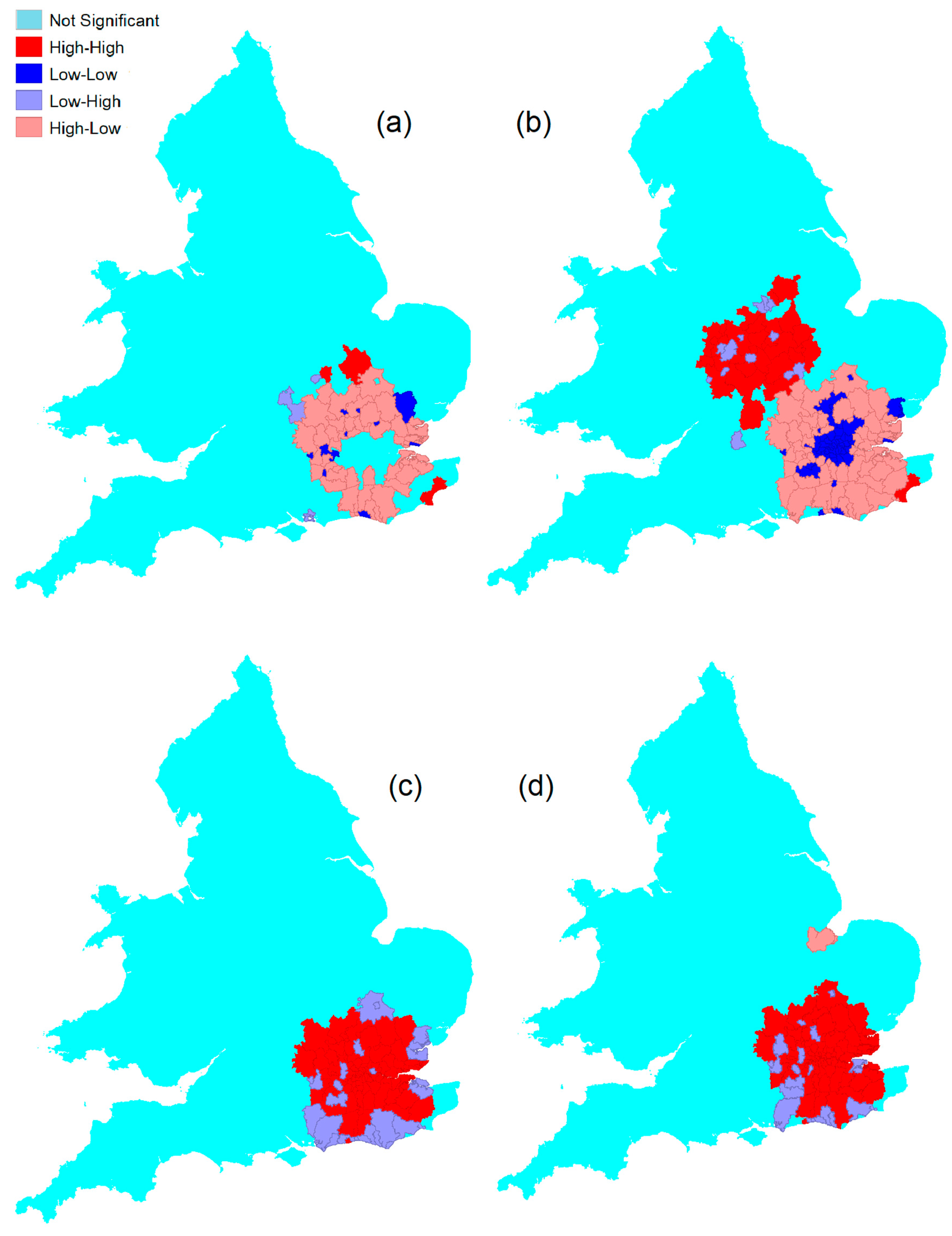
Figure 4.
LISA Maps Migration (25–29; 30–34 and 35–39 years old). (a) Range of 25–29-year-olds in 2012; (b) 30–34 year olds in 2012; (c) 35–39 year olds in 2012; (d) 25–29 year olds in 2018; (e) 30–34 year olds in 2018; (f) 35–39 year olds in 2018.
Figure 4.
LISA Maps Migration (25–29; 30–34 and 35–39 years old). (a) Range of 25–29-year-olds in 2012; (b) 30–34 year olds in 2012; (c) 35–39 year olds in 2012; (d) 25–29 year olds in 2018; (e) 30–34 year olds in 2018; (f) 35–39 year olds in 2018.

Table 1.
Net Migration Rates by working age-band: Regions. The table reports regional net migration rates for English and Welsh regions over nine 5-year age bands. Mean = Mean net migration rate, SD = Standard Deviation.
Table 1.
Net Migration Rates by working age-band: Regions. The table reports regional net migration rates for English and Welsh regions over nine 5-year age bands. Mean = Mean net migration rate, SD = Standard Deviation.
| 20–24 | 25–29 | 30–34 | 35–39 | 40–44 | 45–49 | 50–54 | 55–59 | 60–64 | Mean | SD | |
|---|---|---|---|---|---|---|---|---|---|---|---|
| EE | 6.16 | 1.93 | 6.85 | 6.01 | 2.77 | 0.95 | −0.05 | −0.60 | 0.01 | 2.67 | 2.95 |
| EM | −15.65 | −1.07 | 4.72 | 4.78 | 2.69 | 2.49 | 2.36 | 2.50 | 1.34 | 0.46 | 6.29 |
| LON | 33.78 | 6.53 | −21.41 | −21.87 | −13.88 | −8.82 | −7.18 | −6.64 | −5.63 | −5.01 | 16.93 |
| NE | −15.97 | −5.31 | 0.44 | 0.96 | 1.38 | 1.23 | 1.63 | 2.14 | 2.02 | −1.28 | 5.96 |
| NW | −0.56 | 0.81 | 1.55 | 1.87 | 1.13 | 0.82 | 0.64 | −0.01 | 0.06 | 0.70 | 0.78 |
| SE | −4.68 | −2.27 | 5.82 | 6.44 | 3.69 | 0.64 | −0.71 | −1.33 | −1.56 | 0.67 | 3.83 |
| SW | −9.10 | 2.38 | 5.73 | 5.64 | 4.38 | 3.77 | 4.35 | 5.05 | 5.05 | 3.03 | 4.66 |
| WA | −8.76 | −3.27 | 2.44 | 2.39 | 1.98 | 3.17 | 4.36 | 5.11 | 4.33 | 1.30 | 4.50 |
| WM | −4.51 | −2.01 | 1.13 | 1.04 | 0.94 | 0.59 | 0.02 | 0.04 | −0.05 | −0.31 | 1.84 |
| YH | −12.07 | −4.15 | −0.10 | 0.63 | 0.53 | 0.28 | 0.55 | 0.37 | 0.57 | −1.49 | 4.25 |
EE = East of England, Lon = London, SE = South East, EM = East Midlands, WM = West Midlands, WA = Wales, SW = South West, NE = North East, NW = North West, YH = Yorkshire/Humberside.
Table 2.
LISA combinations migration and house price–earnings ratio. This table reports house price earnings ratios (HPER) and net migration rates (NMR). It also reports the number of districts (LAD) in the cluster, the total population, its average age, and the number of infant migrants.
Table 2.
LISA combinations migration and house price–earnings ratio. This table reports house price earnings ratios (HPER) and net migration rates (NMR). It also reports the number of districts (LAD) in the cluster, the total population, its average age, and the number of infant migrants.
| No. LADs | Population Millions | Migrant 0–4 | NMR 0–4 | Pop/ Sqm | HPER Med | HPER LQ | Age | ||
|---|---|---|---|---|---|---|---|---|---|
| (a) | 0–4 | ||||||||
| NotSig | 186 | 32.63 | 10,058 | 3.08 | 276 | 7.27 | 7.28 | 43.0 | |
| HH | 28 | 3.09 | 3888 | 12.60 | 319 | 8.36 | 8.76 | 43.7 | |
| LL | 52 | 11.16 | −20,127 | −18.04 | 2631 | 13.91 | 14.60 | 36.7 | |
| LH | 17 | 4.47 | −2684 | −6.00 | 2204 | 6.44 | 6.98 | 37.5 | |
| HL | 55 | 7.77 | 8194 | 10.54 | 457 | 12.30 | 13.13 | 42.5 | |
| (b) | HPER | ||||||||
| NotSig | 180 | 29.63 | 9839 | 3.32 | 263.3 | 7.53 | 7.63 | 43.89 | |
| HH | 34 | 8.30 | 986 | 1.19 | 782.5 | 5.99 | 5.76 | 40.50 | |
| LL | 89 | 15.67 | −8806 | −5.68 | 918.1 | 11.95 | 13.19 | 39.65 | |
| LH | 4 | 0.28 | 285 | 10.10 | 105.8 | 6.65 | 7.43 | 46.63 | |
| HL | 31 | 5.24 | −2817 | −5.38 | 640.5 | 14.38 | 13.78 | 40.54 | |
| (c) | Combined | ||||||||
| Other | 237 | 40.91 | 11,762 | 2.88 | 310 | 7.45 | 7.56 | 42.70 | |
| LL0–4 | LLHPER | 38 | 8.24 | −14,846 | −18.01 | 2210 | 12.96 | 14.28 | 36.50 |
| HL0–4 | LLHPER | 37 | 5.49 | 5556 | 10.13 | 568 | 11.85 | 13.12 | 41.74 |
| LL0–4 | HLHPER | 12 | 2.74 | −5319 | −19.40 | 6289 | 17.27 | 15.94 | 36.02 |
| HL0–4 | HLHPER | 14 | 1.73 | 2334 | 13.46 | 333 | 13.63 | 13.43 | 43.11 |
HH: High–High, LL: Low–Low, LH: Low–High, HL: High–Low.
Disclaimer/Publisher’s Note: The statements, opinions and data contained in all publications are solely those of the individual author(s) and contributor(s) and not of MDPI and/or the editor(s). MDPI and/or the editor(s) disclaim responsibility for any injury to people or property resulting from any ideas, methods, instructions or products referred to in the content. |
© 2023 by the author. Licensee MDPI, Basel, Switzerland. This article is an open access article distributed under the terms and conditions of the Creative Commons Attribution (CC BY) license (https://creativecommons.org/licenses/by/4.0/).
Share and Cite
MDPI and ACS Style
Gray, D. What Can District Migration Rates Tell Us about London’s Functional Urban Area? J. Risk Financial Manag. 2023, 16, 89. https://doi.org/10.3390/jrfm16020089
AMA Style
Gray D. What Can District Migration Rates Tell Us about London’s Functional Urban Area? Journal of Risk and Financial Management. 2023; 16(2):89. https://doi.org/10.3390/jrfm16020089
Chicago/Turabian StyleGray, David. 2023. "What Can District Migration Rates Tell Us about London’s Functional Urban Area?" Journal of Risk and Financial Management 16, no. 2: 89. https://doi.org/10.3390/jrfm16020089