
Asymmetric Effects of Financial Development on CO2 Emissions in Bangladesh


1
Department of Economics, Justice, and Policy Studies, Mount Royal University, Calgary, AL T3E 6K6, Canada
2
Finance and Economics, Gary W. Rollins College of Business, University of Tennessee at Chattanooga, Chattanooga, TN 37403, USA
3
School of Management, Economics, and Mathematics, King’s University College at Western University Canada, London, ON N6A 2M3, Canada
*
Author to whom correspondence should be addressed.
J. Risk Financial Manag. 2023, 16(5), 269; https://doi.org/10.3390/jrfm16050269
Submission received: 3 March 2023
/
Revised: 7 May 2023
/
Accepted: 10 May 2023
/
Published: 12 May 2023
(This article belongs to the Special Issue International Trade, Finance, and Development)
Abstract
:Depending on how it functions and is organized, the financial system can have a negative, positive, or zero impact on the environment. For Bangladesh, the empirical relationship between financial development and the environment, measured in terms of carbon dioxide (CO2) emissions per capita, is analysed over the period 1980 to 2020. This is the first such analysis for this country. We perform this within a non-linear bound testing framework while controlling for changes in energy consumption, gross domestic product, and trade volume. There are two key findings. One, we find that the relationship between CO2 emissions per capita and financial development is cointegrating, with the direction of cointegration running from financial development to CO2 emissions. Two, we find that positive and negative changes in financial development have asymmetric impacts on CO2 emissions in the long and short run. The implications of these findings are discussed regarding their attendant environmental policy implications.
JEL Classification:
C22; E44; Q53; Q561. Introduction
In this study, we critically review the issues regarding the relationship between financial development and carbon dioxide (CO2) emissions, elucidate empirically the nature of this relationship for Bangladesh, and discuss the attendant policy implications of our findings. Global CO2 emissions are the most important driver of climate change; the deleterious effects of which are being experienced today. The growth of these emissions, particularly those associated with the burning of fossil fuels, has doubled between 1980 and 2020. CO2 emissions at the end of 2020 reached a high of 35.26 billion tons (Our World in Data 2022a). Asia has accounted for over 50% of global emissions. While Bangladesh, a country in Asia, is not viewed as a major CO2 emitter relative to China and India, it nonetheless contributes to the overall increase in the region’s CO2 emissions. This is mostly due to economic activities involving the continuous burning of fossil fuels and the manufacture of cement in that country. Bangladesh’s CO2 emissions per capita increased from 0.05 tons in 1972 to 0.54 tons in 2020, growing at an average annual rate of just over 5% (Our World in Data 2022a).
The growth in global CO2 emissions has been linked to several factors, including the development of the financial sector. In the 1980s, Bangladesh started a vast and pervasive financial liberalization program to develop its financial sector. The result of which is substantial growth of its banking system. Of note, private credit to GDP has increased significantly since 2003 and microfinance has doubled as a share of GDP (Raihan et al. 2017; World Bank 2022). This increased access to finance through the microfinance sector and private banks have improved living standards for households and increased investment by firms. However, this financial development could be having a negative impact on the environment. For example, with financial development there could be an increase in the consumption of goods and services that rely on production processes that increase CO2 emissions.
Theoretical models suggest that financial development could have positive, negative, or no impact on CO2 emissions. For instance, financial development facilitates greater mobilization of credit to businesses and households for investments and increased consumer spending. If these investments are concentrated in certain techniques of production that utilize greater energy consumption, and if the associated increase in consumer spending is primarily on consumer durables that also utilize greater energy consumption, then CO2 emissions can increase (Ehigiamusoe et al. 2021). In contrast, if these investments are used to develop new energy efficient technologies and promote the use of renewable energy projects, then the impact on CO2 emissions could be nonpositive (Ehigiamusoe et al. 2021). Much of the empirical analysis on the impact of financial development on CO2 emissions assumes no asymmetry. However, this does not need to be the case since positive and negative changes to financial development could have different impacts on CO2 emissions. Changes in the financial system are complex; they involve allocating financial resources more efficiently, improving financial intermediation, and strengthening competition within the private sector. Thus, it is important to allow for equally sized, in absolute terms, positive and negative changes in financial development to potentially have different impacts on CO2 emissions (Shah 2008; Shahbaz et al. 2016).
Our study of the impact of financial development on CO2 emissions per capita in Bangladesh contributes to the literature in three significant ways. One, to the best of our knowledge, this is the first study that focuses only on Bangladesh rather than a study based on this country as part of a group of countries (e.g., Bui 2020; Jiang and Ma 2019). Accordingly, our study provides useful insights on the specific CO2 emissions–financial development relationship for Bangladesh. These insights will be informative for government policymakers designing policies aimed at reducing CO2 emissions and improving environmental sustainability. Second, our study adds to the burgeoning literature on the asymmetric relationship between CO2 emissions and financial development. Our study uses the non-linear autoregressive distributed lags (NARDL) model with annual data over the period 1980 to 2020. We control for confounding factors by including changes in energy consumption, gross domestic product (GDP) per capita, and trade volume. Third, the variable we use to measure financial development is novel. This is a relatively new and comprehensive index developed by Svirydzenka (2016).
There are two important findings. First, we find evidence of a long-term cointegrating relationship running from CO2 emissions per capita to changes in financial development, energy consumption, GDP per capita, and trade volume. Second, we find that positive and negative changes in financial development have asymmetric impacts on CO2 emissions in the short and long run. Our findings echo those by Majeed et al. (2020) and Omoke et al. (2020), among others. Based on these findings, we provide important policy recommendations for Bangladesh. These recommendations could also be of importance for other developing countries that often struggle to maintain a balance between developing their financial sector while ensuring environmental sustainability. One of these policies is to expand the existing green banking policy, and thereby, create incentives for financial institutions to include environmental, social, and corporate governance framework in their financial portfolios.
The rest of the paper proceeds as follows. Section 2 first provides an overview of the financial development in Bangladesh. This section then evaluates the existing empirical literature on the relationship between financial development and CO2 emissions. Section 3 discusses the data and methods. Section 4 presents our findings and Section 5 discusses them. Section 6 concludes with a summary and the attendant policy implications.
2. Literature Review
2.1. Financial Development in Bangladesh and the Sustainable Finance Policy
In the first decade after its independence in 1971, Bangladesh’s financial sector was characterized by weak institutions. This weakness resulted in a substantial amount of non-performing loans and growing calls for financial sector reform. The financial sector reform, which encompassed financial liberalization, took place in three phases. The first phase was in the 1980s. In this period, there was a denationalization of public banks, development of new private banks, and the establishment of the National Commission on Money, Banking, and Credit (Uddin et al. 2014). The second phase of the reform began in the early 1990s. In this phase, there were several initiatives. The primary goals of these were to enhance financial intermediation and productivity and to increase competitiveness of the banking sector through a series of legal, policy, and institutional reforms (Shah 2008). Some of these initiatives included allowing for market-determined interest rates, giving greater autonomy to the central bank of Bangladesh, expanding supervision skills of the central bank, and improving the legal and judicial processes to ensure debt recovery. The final phase of the reform took place in the late 1990s. In this phase, the capital market was liberalized by removing some restrictions in capital movements.
Although Bangladesh has a long history of policy reform in the financial sector, adopting environmentally friendly practices in this sector is new. This makes Bangladesh an intriguing case to study whether reforms in the financial sector have had negative environmental impacts. In 2011, Bangladesh Bank undertook several green banking initiatives to support environmentally responsible financing. More recently, in 2020, Bangladesh Bank introduced the Sustainable Finance Policy to encourage socially responsible financial policy with respect to sustainability (Bangladesh Bank 2020). The goal of this policy is to encourage financial institutions to contribute to and participate in a conditional 15% reduction in CO2 emissions by 2030. A few aspects of the Sustainable Finance Policy are worth noting: (i) monitoring a client’s environmental, social, and corporate governance performance to ensure emissions are below permitted limits; (ii) financing technological innovation that minimizes waste, emissions, and reduce materials and energy inputs; (iii) implementing green banking polices that foster environmentally responsible financing practices; (iv) collecting data on carbon footprints of the commercial banks and other financial institutions; and (v) directing financing and equity investment to companies that undertake emission reduction projects and programs. The full impact of these policies is yet to be determined. However, their impact will partly depend on the level of emissions by the financial sector.
2.2. Empirical Literature on Financial Development and Emissions
The studies on the impact of financial development on CO2 emissions have produced contradictory findings, with some scholars reporting negative, positive, or no impact. Many of these studies proceed on the assumption the impact of financial development on CO2 emissions is symmetric. Shahbaz et al. (2013b), in a study on Malaysia for the period 1971 to 2011 for instance, utilized the autoregressive distributed lags bounds (ARDL) framework and found that financial development reduces CO2 emissions. In a later study on France, Shahbaz et al. (2018), examined the impact of financial development—measured as per capita real domestic credit to the private sector—on CO2 emissions and found a similar result. Using the ARDL technique, other scholars found comparable results. These include Abbasi and Riaz (2016) for Pakistan; Jalil and Feridun (2011) for China; and Nasreen et al. (2017) for several South Asian economies. In the case of panel studies, Tamazian et al. (2009) examined the relationship between financial development and CO2 emissions for the BRICS economies. They found financial liberalization and openness mitigated against environmental degradation, that is, it reduces CO2 emissions. In an extension of this study, Tamazian and Rao (2010) examined the same relationship for a group of 24 transitional economies and found similar results. Likewise, Al-Mulali et al. (2015) and Hao et al. (2016) confirmed similar findings. These findings of a negative impact of financial development on CO2 emissions are indicative of an overall improvement in environmental quality.
Other studies have established a positive relationship between financial development and CO2 emissions. Several of these studies have highlighted various conduits through which this can occur. One, they contended that a more laxed financial system can loosen households’ budget constraints. This loosening can induce increases in CO2 emissions when there is an associated increase in demand for consumer durables, such as appliances, cars, and machinery. Two, an improved financial system can mean greater access to cheaper capital for firms and businesses. Their investments in production techniques that do not utilize green technology can cause increasing levels of CO2 emissions. For instance, Omoke et al. (2020), investigated the effect of financial development on CO2 emissions in Nigeria using the ARDL technique. Their result was that financial development has a positive impact on CO2 emissions. Using the ARDL method, other scholars found a positive impact of financial development on CO2 emissions including Cetin et al. (2018) for Turkey; Shahbaz et al. (2015) for India; Shahbaz et al. (2016) for Pakistan; Abbasi and Riaz (2016) for Pakistan; Zhang (2011) for China; and Maji et al. (2017) for Malaysia. Similarly, among panel studies, the presence of a positive relation is established by these scholars: Bekhet et al. (2017); Hao et al. (2016); Acheampong (2019); Acheampong et al. (2020); Gök (2020); and Ehigiamusoe and Lean (2019).
Still, some studies report no impact of financial development on CO2 emissions. That is, they could not confirm a statistically significant relationship between financial development and CO2 emissions. For example, Jiang and Ma (2019) applied the generalized method of moments technique to a panel of developed countries from 1960 to 2010. They found that financial development has no impact on CO2 emissions. Charfeddine and Kahia (2019) found that financial development had almost no impact on CO2 emissions in a majority of 24 MENA countries for the period 1980 to 2015. Similar results were also found by Omri et al. (2015) for a panel of 12 MENA countries and Jamel et al. (2017) for a panel of 40 European countries.
2.3. Asymmetry between Financial Development and CO2 Emissions
The differing results on the relationship between financial development and CO2 emissions indicate that this issue is far from settled. Along this vein, a few scholars have explored the possibility of an asymmetric relationship between the variables, wherein positive and negative shocks to financial development may have different impacts on CO2 emissions. To that end, Omoke et al. (2020) utilized the NARDL technique on data for Nigeria from 1971 to 2014. With impacts measured in absolute terms, they found that a negative shock to financial development led to a larger increase in CO2 emissions than a positive shock to financial development led to a decrease in CO2 emissions. Similarly, Brown et al. (2022) investigated asymmetric impacts of financial development on CO2 emissions for Jamaica from 1980 to 2018. Using the NARDL method, they found that the impact of financial development on CO2 emissions was asymmetric in the short and long run. Majeed et al. (2020) utilized a similar technique using annual data for Pakistan from 1972 to 2018. They too found an asymmetric relationship between financial development and CO2 emissions. Other scholars that have found asymmetric impacts include Lahiani (2020) for China, and Boufateh and Saadaoui (2020) for 22 African countries.
The review of the existing literature on the asymmetric nature of the impact of financial development on CO2 emissions remains an active area of research since the evidence reported thus far is conflicting. Consequently, there is no a priori empirical certainty regarding the nature of the impact of financial development on CO2 emissions, which therefore indicates that further work needs to be conducted in this area. Accordingly, we examine for the first time the impact of financial development on CO2 emissions for the Bangladesh economy.
3. Data and Methods
3.1. Data
The data are annual and span the period 1980 to 2020. We define as CO2 emissions measured in tonnes per person. The data on were obtained from Our World in Data (2022a). is per capita primary energy consumption. It is measured in kilowatt-hours per person and was obtained from Our World in Data (2022b). is GDP per capita (per person), measured in constant 2015 USD. is the volume of trade and is the sum of exports and imports, both also measured in constant 2015 USD. and were obtained from the World Bank (2022). is the financial development index developed by the International Monetary Fund (2022) based on the work of Svirydzenka (2016). This index accounts for the size and depth of the financial markets, the stability and efficiency of the financial system, the accessibility of financial services, and the level of financial innovation. Figure 1 shows the historical evolution of financial development and CO2 emissions in Bangladesh from 1980 to 2020.
Regarding the choice of the variables that are used to model the dynamics of , this choice is made based on a thorough review of the theoretical and empirical literature. For GDP and energy consumption, Ang (2007, 2008), Soytas et al. (2007), Zhang and Cheng (2009), Chang (2010), and Shahbaz et al. (2013a, 2013b), among others, have identified these variables as important determinants of CO2 emissions. In general, increases in national income and energy consumption are likely to contribute to pollution. With respect to financial development as a determinant of CO2 emissions, some of the recently published empirical studies have been noted in the literature review above. Effects of trade volume on CO2 emissions can be traced back to Grossman and Krueger (1995). They postulated that the ultimate effect of openness on the environment depends on how and what policies are implemented in a country. Shahbaz et al. (2013a) discussed two schools of thought on the relationship between trade and openness. One way to look at the trade effect on the environment is that international trade creates competition among countries and provides countries with access to the international market. To remain competitive, developing countries are encouraged to choose the most efficient technology and import cleaner technology from developed countries. Thus, the link between international trade and emissions could very well be positive. Contrarily, international trade can deplete natural resources and intensify emissions. Regardless of what the impact of openness on CO2 emissions may be, it is imperative to include some measure of international trade as an independent variable while modelling CO2 emissions.
3.2. Methods
We begin by applying the logarithmic transformation to , , , , and . They are denoted as , , , , and , respectively. To examine the long- and short-run dynamics and asymmetries between CO2 emissions and financial development in Bangladesh, we apply bounds testing using NARDL. This framework was proposed by Shin et al. (2014) to explore whether there is a hidden cointegration among the variables (Granger and Yoon 2002). The NARDL model is a straightforward, yet powerful, way to simultaneously analyse short-run and long-run asymmetries among variables for a few reasons. With a well-specified model, one can solve the problems of serial correlation of the errors and endogeneity of the regressors if it exists (Kanas and Kouretas 2005). The model is flexible in accommodating combinations of I(1) and I(0) variables. Furthermore, the NARDL model is well suited for small samples, such as ours. Its single equation setup means fewer degrees of freedom are lost and that there is greater power in statistical testing when compared to system of equations modelling setups.
To start the NARDL, we first decompose into its positive and negative partial cumulative sums. These are denoted as and , respectively. They are calculated as shown in Equations (1) and (2), respectively.
Before applying the NARDL technique, we verify if the variables have an order of integration that is no greater than one. In this regard, we use the Augmented Dickey–Fuller (ADF) test to confirm the order of the integration of the variables. If none of the variables has an order of integration greater than one, then we can apply the NARDL. The NARDL model, where is the dependent variable, is estimated by way of an unrestricted (unconstrained) error correction model. This incorporates the short-run (the first differences) and long-run (the levels) dynamics among the variables as shown in Equation (3).
The lags , , , , and are selected based on the Akaike information criterion so that the residuals, the estimate of the error term , are well-behaved. In this regard, we verify that the residuals of the chosen NARDL model are serially uncorrelated, normally distributed, and homoscedastic using the Jarque–Bera Normality, Breusch–Godfrey Serial Correlation Lagrange Multiplier, and Breusch–Pagan–Godfrey Heteroskedasticity tests, respectively.
The Jarque–Bera Normality test evaluates whether the residuals have third (skewness) and fourth (kurtosis) moments about the mean that match those of the normal distribution (Jarque and Bera 1980). The null hypothesis is that the residuals are normally distributed. The Breusch–Godfrey Serial Correlation Lagrange Multiplier is a test of serial correlation of the residuals, with the null hypothesis being no serial correlation (Breusch 1978; Godfrey 1978). The Breusch–Pagan–Godfrey Heteroskedasticity tests is based on the work of Breusch and Pagan (1979). It tests whether the residuals have constant variance, with the null hypothesis of this test being homoskedasticity. In addition, for the chosen NARDL, we test for functional misspecification (omitted dynamics) by using the Ramsey Regression Equation Specification Error Test (RESET) proposed by Ramsey (1969). This misspecification is assessed with respect to the first order. To do this, we first calculate from the NARDL model the square of fitted values of the dependent variable. We then include the square of the fitted values in the original NARDL model as a regressor, and then re-estimate the NARDL model. If the coefficient on the square of the fitted value is statistically significant, then we have misspecification of some kind, and our model is not statistically adequate. The null hypothesis of the Ramsey RESET test is no functional form misspecification.
Finally, we test that the NARDL’s cumulative sum (CUSUM) of the recursive residuals and the CUSUM of squares of recursive residuals do not indicate statistical evidence at the 5% significance level of parameter and/or variance instability. The CUSUM of the recursive residuals and the CUSUM of the squares of recursive residuals are based on forward recursion and are calculated following Brown et al. (1975).
The NARDL bounds testing is essentially a check of whether Equation (3) better captures the dynamics among the variables against a model that captures only the short-run dynamics as shown in Equation (4).
To establish whether Equation (3) or Equation (4) properly captures the dynamics among the variables, we first perform bounds testing. Bounds testing involves first estimating Equation (3) and then conducting an F-test and a t-test. These tests are non-standard, having their own bootstrapped critical values for various sample sizes. At various levels of statistical significance, these tests have upper and lower bound critical values, named I(1) and I(0), respectively. For the F-test, the null hypothesis is that , and the alternative hypothesis is that at least one of these parameters is non-zero. The decision regarding the rejection of the null hypothesis is made on the basis of I(1) and I(0) critical values at various levels of statistical significance and sample sizes as tabulated by Pesaran et al. (2001). At a chosen statistical significance level, when the F-test statistic is greater than the I(1) critical value, we reject the null hypothesis of evidence against a long-run level and cointegrating relationship. On the other hand, if the F-test statistic is below the I(0) critical value, this is evidence against cointegration. Where the F-test statistic is between the I(1) and I(0) critical values, the test is inconclusive. Should we reject the null hypothesis of the F-test, then a bounds t-test is performed. The null hypothesis of the t-test is that and the alternative hypothesis mostly commonly stated is that . However, to be technically correct we are conducting a one-sided t-test with the alternative hypothesis being that For a full and accessible discussion, the interested reader can review Kripfganz and Schneider (2020, 2023). The test also has its own I(1) and I(0) critical values at various levels of statistical significance (see also Pesaran et al. 2001). We reject the null hypothesis if the absolute value of the t-test statistic is greater than the absolute value of the t-test I(1) critical value.
To assess asymmetry, we use a Wald test (Wald 1945). For short-run asymmetry, the null hypothesis is that the addition of the coefficients of the first differences of the positive partial sums is equal to the addition of the first differences of the negative partial sums, namely, . The alternative hypothesis is that they are not equal. Regarding long-run asymmetry, the null hypothesis is that the coefficients on the levels of the positive and negative partial sums are equal, that is . The alternative hypothesis is that they are not equal. In addition to the Wald test, we conclude our examination of asymmetry with the dynamic multiplier graph of the long-run impact of changes in financial development on CO2 emissions per capita.
We remark on four reasons why we apply the logarithmic transformation to all the variables in the NARDL model. One, the coefficient of a natural logarithmic transformed independent variable is the elasticity of the raw (untransformed) dependent variable with respect to the raw independent variable. Two, we will have a more complicated multiplicative model, which may be a more realistic way of modelling the dynamics among our variables. Three, applying a logarithm to our variables makes them more homoscedastic by suppressing and stabilizing their variances. Four, the logarithmic transformation improves the fit of the dataset to the model wherein the error term will have distributional features closer to the normally shaped bell curve. For small samples such as ours, this will be important for making valid statistical inferences (DasGupta 2008).
As a robustness check of the inference to be drawn from the NARDL model, we test for constancy of the cointegrating relationship produced by this model over the 0.25, 0.5, and 0.75 quantile limits by estimating a quantile autoregressive distributed lag (QARDL) model. This estimation that is based on the chosen NARDL model is given by Equation (3).1 The first test based on this QARDL is the quantile slope equality that is grounded on Koenker and Bassett (1982). The null hypothesis of this test is that the coefficients on the variables across the quantiles are equal. The second is the Newey and Powell (1987) test of conditional symmetry. Its null hypothesis is that the average of the coefficient values on the variables for symmetric quantiles around the median are, statistically speaking, equal to value of the coefficients on the variables at the median.
4. Results
4.1. Unit Root Test
The results of the ADF unit root test on the first difference and levels of the variables are presented in Table 1. For the level variables, the null hypothesis that the series has a unit root is not rejected at the conventional level of statistical significance. However, the same null hypothesis is rejected at the 1% level of statistical significance for all variables when the test is applied to their respective first differences. Therefore, we find that no variable is integrated to an order of more than one. These results allow us to proceed with the NARDL bounds test.
4.2. NARDL Bounds Tests and Model Diagnostics
The F-test and t-test statistics estimated from the NARDL model are presented in Table 2. The value of the F-test statistic is 9.82, which is higher than the I(1) value of 4.68 at the 1% level of statistical significance. We find that the value of the t-test statistic (−7.16) is lower than the I(1) critical value (−4.79) at the 1% level of statistical significance. Therefore, according to both these tests, we reject the null hypothesis that there is no evidence of a long-run level cointegrating relationship running form , , , , and LNTRADE to .
The NARDL bounds testing and the inference that we make rely on the statistical adequacy of the NARDL model. As such, diagnostic tests are crucial to confirm statistical adequacy. These diagnostic tests are reported in Table 3, and Figure 2 and Figure 3. The results in Table 3 indicate that the residuals are normally distributed, homoscedastic, and serially uncorrelated. From this table, the Ramsey RESET test result indicates that the NARDL model is not misspecified in the first order wherein the powers of the fitted values of the dependent variable would have explanatory power. Figure 2 and Figure 3 show the CUSUM of recursive residuals and the CUSUM squares of recursive residuals. These figures indicate that there is no variance or parameter instability at the 5% level of statistical significance. This is because both recursive residuals lie within their respective 5% significance bands.
4.3. NARDL Long-Run and Short-Run Models
We present the long-run level and short-run equations in Table 4. As expected, the coefficient on is positively associated with . This coefficient is statistically significant at the 1% level. Its value indicates that a 1% increase in energy consumption per capita is associated with a 0.81% increase in CO2 emission per capita in the long run. This result is in line with earlier findings by Alam et al. (2012). Regarding the impact of in the long-run equation, it is not statistically significant at conventional levels. On the other hand, the coefficient on is negative and statistically significant at the 5% level. At first glance, this result might seem counterintuitive. However, as previous studies have suggested, a negative per capita income in the CO2 equation is plausible. For example, rising levels of GDP could be associated with increased ecological awareness, adoption of new green technologies, and utilization of alternative energy sources (Muhammad 2019; Salazar-Núñez et al. 2020; Ceretta and Vieira 2021). This is particularly true for Bangladesh. As noted by Khandker et al. (2014) and Das et al. (2021), among developing countries, Bangladesh is a success story in the adoption of relatively new solar technology. Of note, as income rose between 2003 and 2014, over 3 million rural homes were using off-grid solar home systems and moved towards environmentally friendly technology.
We now turn our attention to financial development, which is decomposed into its rising and falling partial cumulative sums. From the long-run equation in Table 3, the coefficient of is 0.17 and statistically significant at the 1% level. This value indicates that a 1% increase in the financial development index is associated with a 0.17% rise in CO2 emissions per capita in the long run. Thus, improvements in financial development tend to be associated with rising levels of CO2 emissions in the long run. The coefficient on is 0.12 but statistically insignificant at even the 10% level. Thus, it seems that deleterious changes in financial development do not significantly, statistically speaking, impact CO2 emissions per capita in the long run.
We now formally check if there exist long-run and short-run asymmetry by applying the Wald test of coefficient restrictions. The long-run and short-run Wald χ2-test results are shown at the bottom part of Table 4. For the long run, the χ2-test statistic is 5.39 and statistically significant at the 5% level. Regarding the short run, the χ2-test statistic is 10.75 with statistical significance at the 1% level. Therefore, we conclude that an asymmetric relationship exists between financial development and CO2 emissions in the long run and short run. These findings agree with studies in the recent literature on other countries by Ling et al. (2022), Lahiani (2020), Majeed et al. (2020), and Omoke et al. (2020). Another way to examine asymmetry is to look at the dynamic multiplier graph of the long impact of a one percent change in and on . Figure 4 shows this graph and confirms the asymmetry findings. We observe that the impact of positive changes in financial development dominates the impact of negative changes on CO2 emissions per capita in the long run. Therefore, what we find from our results is that an increase in financial development perhaps incentivizes pollution-creating activities; however, a decrease in financial development does not significantly change emissions.
4.4. Robustness
We now conduct a robustness check of the inference made about the long- and short-run asymmetries from the NARDL model by applying a quantile re-estimation of this model. We do not report here the full results of this quantile model, but these are available upon request. Based on the results of the quantile model, what we present here is the Koenker and Bassett (1982) test of coefficient equality and Newey and Powell (1987) test of conditional symmetry at the 0.25, 0.5, and 0.75 quantile limits. These test results are shown in Table 5. We focus on the coefficients of the error correction term, positive partial cumulative sums, and the negative partial cumulative sums. From this table, we find based on the Wald test statistics for the equality and conditional symmetry coefficients that there are no statistically significant differences across quantiles. The probability values associated with the test statistics are all greater than the 10% level.
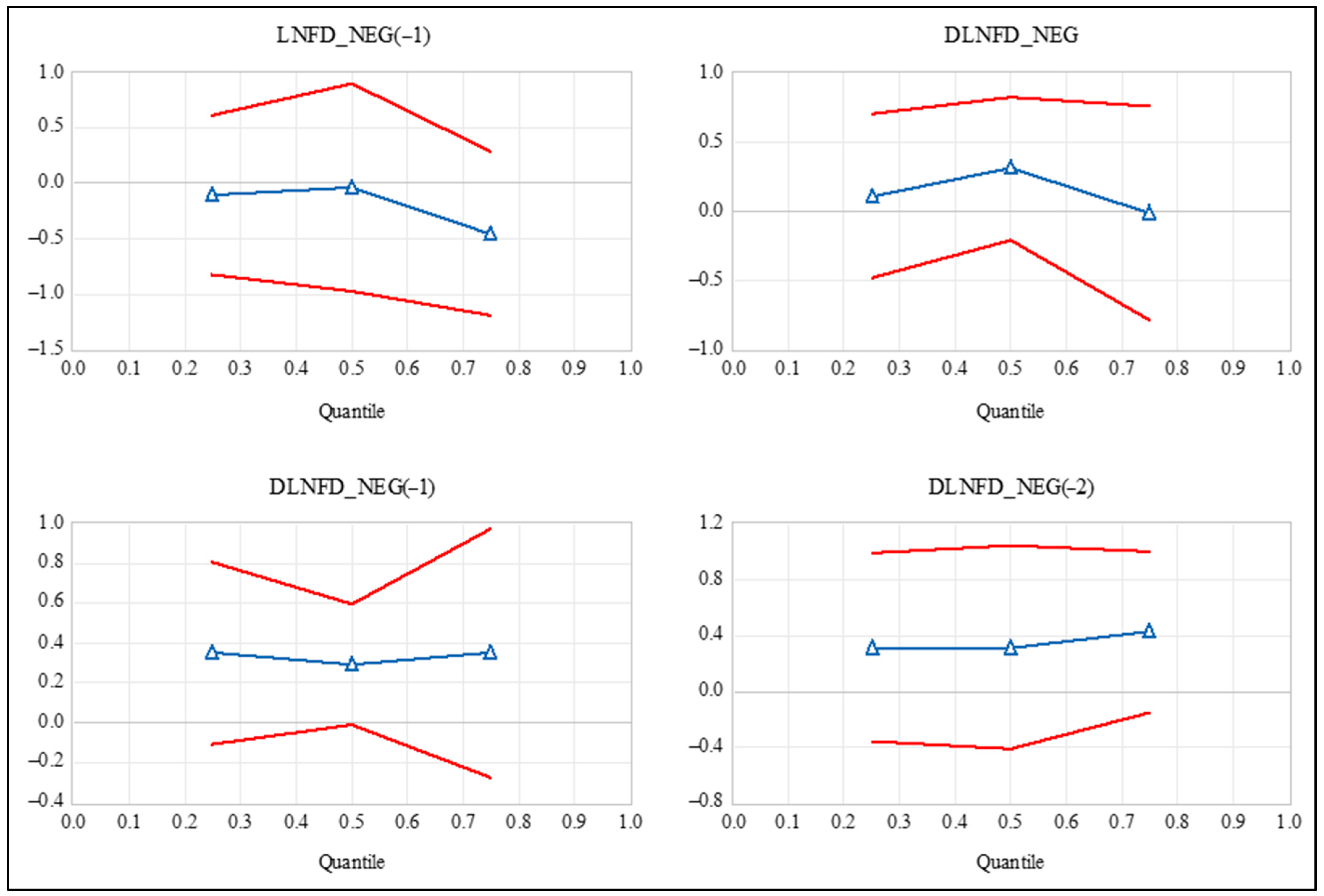
Figure 5, Figure 6 and Figure 7 provide a visual perspective from which to assess stability of the coefficient values on the error correction term, positive partial cumulative sums, and negative cumulative sums, respectively. These figures show the coefficient values at the 0.25, 0.5, and 0.75 quantile limits alongside their respective 95% confidence intervals. From these figures, we observe generally that there is stability of the coefficients across the quantiles, consistent with Koenker and Bassett (1982) and the Newey and Powell (1987) test results of no statistically significant differences in coefficients across quantiles. We do note that there is some overcorrection with respect to the error correction term in the upper quantile, but this is small and indicates an oscillatory pattern to equilibrium in the long run. Thus, we conclude that the NARDL model is robust and statistically adequate with respect to characterizing the long-run and short-run equilibrium asymmetric cointegrating relationship among our variables.
5. Discussion
Overall, there are two important findings. First, we find evidence of long-run cointegration running from financial development to CO2 emissions. Second, we find that positive and negative changes in financial development have asymmetric impacts on CO2 emissions in the long and short run. These findings for Bangladesh are consistent with studies on other countries. For instance, Brown et al. (2022) and Majeed et al. (2020) all found evidence of asymmetry between these variables for Jamaica and Pakistan, respectively. A common feature among these countries and Bangladesh is that they all had poorly functioning financial systems in place that retarded their long-term growth and development. For example, in Jamaica, there was limited competition in the financial sector since there were only a few private banks. This lack of competition essentially gave these banks monopoly-like power over the financial sector. This led to banks charging arbitrarily high interest rates to the detriment of investment and economic growth. In addition, they also had controls including high reserve requirement, interest rate controls, low and negative real interest rates, as well as a severely underdeveloped financial market that failed to transfer funds from people with an excess of those funds to people without funds, but who may have had profitable investment ideas (Brown et al. 2022). The removal of these controls, it is argued, have allowed for a better functioning financial sector that could accelerate economic growth.
A similar situation existed in Pakistan in that the financial sector was not meeting the objective of channelling funds efficiently to encourage financial productivity. However, in the late 1980s, that country embarked upon a financial liberalization program that involved interest rate deregulation, privatization, monetary management, the removal of barriers to entry, banking reforms, improvement of the legal and judiciary process to ensure debt recovery, capital and stock market development, among others (Idrees et al. 2022). The removal of these controls has had beneficial impacts on the financial sector in that country with significant expansion of stock market capitalization, private credit to GDP ratio, and the money supply to GDP ratio. More specifically, the price of financial services is now market-determined, which has had an immense impact on encouraging private sector credit expansion.
Bangladesh, like Jamaica and Pakistan, had several crippling financial controls in place that also prohibited the growth and development of its financial sector, and by extension the economy. However, the extensive liberalization process started by that country in the 1980s saw several of these controls either relaxed or removed completely. These included market-determined interest rates, greater autonomy to the central bank of Bangladesh, the expansion of supervision skills of the central bank, and the improvement of the legal and judicial processes to ensure debt recovery and to develop a more robust and stable financial system conducive to economic growth. According to Uddin et al. (2014), the removal of these restrictions may be responsible for the impressive growth the country has enjoyed since the 2000s.
In summary, the finding that positive and negative shock to financial development has differential effects on the environment of these economies has highlighted that continuous improvements in financial development can reduce environmental degradation. However, following arguments on conservation policies in Bangladesh (see for example, Das et al. 2013, 2021), we suggest that policymakers need to make a concerted effort to implement strategies that also limit the impact of economic growth on CO2 emissions, since financial development can positively impact economic growth.
6. Conclusions and Policy Suggestions
We examine the impact of financial development on CO2 emissions for Bangladesh. We use annual data for the period 1980 to 2020 and the NARDL bounds testing approach to cointegration. After accounting for changes in energy consumption per capita, GDP per capita, and trade volume, we arrive at two main findings. First, we find that cointegration exists and it runs from financial development to CO2 emissions. Second, we find that positive and negative changes in financial development have asymmetric impacts on CO2 emissions in the long and short run. While our findings rely on several statistical assumptions, they have important policy implications for countries like Bangladesh that have had their financial sector go through a comprehensive financial reform. Based on our findings, we posit that policymakers should prioritize green and environmentally friendly projects. Some sectors have already started this transformation into an environmentally friendly industry. For example, as noted by Awal et al. (2021), Bangladesh has the highest number of green readymade garment factories. This country currently hosts 9 of the world’s top 10 green garment factories. Awal et al. (2021) further argued that a green garment factory reduces energy consumption by 40% and water consumption by over 30%. Therefore, to encourage a transformation towards a green economy, more incentives can be provided to industries that establish green factories.
Furthermore, Bangladesh is still heavily dependent on fossil fuels to generate electricity. The credit market in Bangladesh has been regulated by the Bank Company Law. Banks are allowed to lend a borrower up to 25% of its regulatory capital. However, in November 2022, the central bank of Bangladesh removed this constraint for power plants, who are now allowed to apply for loans of any amount (bdnews24.com 2022). This implies that without any cap, firms are now more likely to borrow and invest in fossil fuels to generate electricity. Such a policy may encourage power plants to use more fossil fuels and increase production, thereby having a detrimental impact on the environment. Instead, we echo Awal et al. (2021) and argue that the Bangladeshi government could give tax breaks, reduce import duties, and provide subsidies to businesses that build green industries. To have a better understanding of the impact of financial development on environmental quality, future studies can consider using other types of pollution indicators such as the total particulate matter and ecological footprints. Further research can also investigate whether financial innovation has any role to play in affecting pollution.
Author Contributions
A.D.: Conceptualizing, data collecting, conducting estimations, writing, revising, reviewing, and proof reading. L.B.: Reviewing the literature, conceptualizing, and writing. A.M.: Revising, directing, and finalizing the writing of the data and methodology. Conducting estimations and conceptualizations related to writing, revising, and finalizing results. Preparing, revising, and finalizing and tables, and figures. Reviewing, proofreading, and editing drafts of the manuscript. All authors have read and agreed to the published version of the manuscript.
Funding
The research received no external funding.
Data Availability Statement
Data is publicly available.
Conflicts of Interest
The authors declare no conflict of interest.
| 1 | Details of the mechanics of the quantile autoregressive distributed lag model can be found in Cho et al. (2015) for the interested reader. |
References
- Abbasi, Faiza, and Khalid Riaz. 2016. CO2 emissions and financial development in an emerging economy: An augmented VAR approach. Energy Policy 90: 102–14. [Google Scholar] [CrossRef]
- Acheampong, Alex O. 2019. Modelling for insight: Does financial development improve environmental quality? Energy Economics 83: 156–79. [Google Scholar] [CrossRef]
- Acheampong, Alex O., Mary Amponsah, and Elliot Boateng. 2020. Does financial development mitigate carbon emissions? Evidence from heterogeneous financial economies. Energy Economics 88: 104768. [Google Scholar] [CrossRef]
- Alam, Mohammad Jahangir, Ismat Ara Begum, Jeroen Buysse, and Guido Van Huylenbroeck. 2012. Energy consumption, carbon emissions and economic growth nexus in Bangladesh: Cointegration and dynamic causality analysis. Energy Policy 45: 217–25. [Google Scholar] [CrossRef]
- Al-Mulali, Usama, Chor Foon Tang, and Ilhan Ozturk. 2015. Does financial development reduce environmental degradation? Evidence from a panel study of 129 countries. Environmental Science and Pollution Research 22: 14891–900. [Google Scholar] [CrossRef]
- Ang, James B. 2007. CO2 emissions, energy consumption, and output in France. Energy Policy 35: 4772–78. [Google Scholar] [CrossRef]
- Ang, James B. 2008. Economic development, pollutant emissions and energy consumption in Malaysia. Journal of Policy Modeling 30: 271–78. [Google Scholar] [CrossRef]
- Awal, Md Hossan, Md Aliullah, and Shishir Saidy. 2021. Green revolution in ready made garments in Bangladesh: An analytical study. International Journal of Engineering and Management Research 11: 22–29. [Google Scholar] [CrossRef]
- Bangladesh Bank. 2020. Sustainable Finance Policy for Banks and Financial Institutions. Dhaka: Bangladesh Bank. [Google Scholar]
- bdnews24.com. 2022. Bangladesh Allows Power Plants to Loan Any Amount from Banks Amid Energy Crisis. bdnews24.com. July 26. Available online: https://bdnews24.com/business/hegot77t9u (accessed on 11 February 2023).
- Bekhet, Hussain Ali, Ali Matar, and Tahira Yasmin. 2017. CO2 emissions, energy consumption, economic growth, and financial development in GCC countries: Dynamic simultaneous equation models. Renewable and Sustainable Energy Reviews 70: 117–32. [Google Scholar] [CrossRef]
- Boufateh, Talel, and Zied Saadaoui. 2020. Do asymmetric financial development shocks matter for CO2 emissions in Africa? A nonlinear panel ARDL-PMG approach. Environmental Modelling & Assessment 25: 809–30. [Google Scholar]
- Breusch, Trevor S. 1978. Testing for autocorrelation in dynamic linear models. Australian Economic Papers 17: 334–55. [Google Scholar] [CrossRef]
- Breusch, Trevor S., and Adrian R. Pagan. 1979. A simple test for heteroscedasticity and random coefficient variation. Econometrica 47: 1287–94. [Google Scholar] [CrossRef]
- Brown, Leanora, Adian McFarlane, Anupam Das, and Kaycea Campbell. 2022. The impact of financial development on carbon dioxide emissions in Jamaica. Environmental Science and Pollution Research 29: 25902–15. [Google Scholar] [CrossRef]
- Brown, Robert L., James Durbin, and James M. Evans. 1975. Techniques for Testing the Constancy of Regression Relationships over Time. Journal of the Royal Statistical Society. Series B (Methodological) 37: 149–92. [Google Scholar] [CrossRef]
- Bui, Duy Tung. 2020. Transmission channels between financial development and CO2 emissions: A global perspective. Heliyon 6: e05509. [Google Scholar] [CrossRef]
- Ceretta, Paulo Sérgio, and Marco Aurélio Vieira. 2021. CO2 emissions: A dynamic structural analysis. Revista de Administração da UFSM 14: 949–66. [Google Scholar]
- Cetin, Murat, Eyyup Ecevit, and Ali Gokhan Yucel. 2018. The impact of economic growth, energy consumption, trade openness, and financial development on carbon emissions: Empirical evidence from Turkey. Environmental Science and Pollution Research 25: 36589–603. [Google Scholar] [CrossRef] [PubMed]
- Chang, Ching-Chih. 2010. A multivariate causality test of carbon dioxide emissions, energy consumption and economic growth in China. Applied Energy 87: 3533–37. [Google Scholar] [CrossRef]
- Charfeddine, Lanouar, and Montassar Kahia. 2019. Impact of renewable energy consumption and financial development on CO2 emissions and economic growth in the MENA region: A panel vector autoregressive (PVAR) analysis. Renewable Energy 139: 198–213. [Google Scholar] [CrossRef]
- Cho, Jin Seo, Tae-hwan Kim, and Yongcheol Shin. 2015. Quantile cointegration in the autoregressive distributed-lag modeling framework. Journal of Econometrics 188: 281–300. [Google Scholar] [CrossRef]
- Das, Anupam, Adian A. McFarlane, and Murshed Chowdhury. 2013. The dynamics of natural gas consumption and GDP in Bangladesh. Renewable and Sustainable Energy Reviews 22: 269–74. [Google Scholar] [CrossRef]
- Das, Anupam, Adian McFarlane, and Luc Carels. 2021. Empirical exploration of remittances and renewable energy consumption in Bangladesh. Asia-Pacific Journal of Regional Science 5: 65–89. [Google Scholar] [CrossRef]
- DasGupta, Anirban. 2008. Asymptotic Theory of Statistics and Probability. New York: Springer. [Google Scholar]
- Ehigiamusoe, Kizito Uyi, and Hooi Hooi Lean. 2019. Effects of energy consumption, economic growth, and financial development on carbon emissions: Evidence from heterogeneous income groups. Environmental Science and Pollution Research 26: 22611–24. [Google Scholar] [CrossRef] [PubMed]
- Ehigiamusoe, Kizito Uyi, Vinitha Guptan, and Suresh Narayanan. 2021. Rethinking the impact of GDP on financial development: Evidence from heterogeneous panels. African Development Review 33: 1–13. [Google Scholar] [CrossRef]
- Godfrey, Leslie G. 1978. Testing against general autoregressive and moving average error models when the regressors include lagged dependent variables. Econometrica 46: 1293–301. [Google Scholar] [CrossRef]
- Gök, Adem. 2020. The role of financial development on carbon emissions: A meta regression analysis. Environmental Science and Pollution Research 27: 1–19. [Google Scholar] [CrossRef]
- Granger, Clive W. J., and Gawon Yoon. 2002. Hidden Cointegration. Economics Working Paper, 2002-02. Los Angeles: University of California. Available online: https://papers.ssrn.com/sol3/papers.cfm?abstract_id=313831 (accessed on 3 February 2023).
- Grossman, Gene M., and Alan B. Krueger. 1995. Economic growth and the environment. Quarterly Journal of Economics 110: 353–77. [Google Scholar] [CrossRef]
- Hao, Yu, Zong-Yong Zhang, Hua Liao, Yi-Ming Wei, and Shuo Wang. 2016. Is CO2 emission a side effect of financial development? An empirical analysis for China. Environmental Science and Pollution Research 23: 21041–57. [Google Scholar] [CrossRef]
- Idrees, Muhammad, Umar Hayat, Magdalena Radulescu, Md Shabbir Alam, Abdul Rehman, and Mirela Panait. 2022. Measuring the financial lineralization index for Pakistan. Journal of Risk and Financial Management 15: 57. [Google Scholar] [CrossRef]
- International Monetary Fund. 2022. Financial Development Index Database. Washington, DC: International Monetary Fund. Available online: https://data.imf.org/?sk=F8032E80-B36C-43B1-AC26-493C5B1CD33B (accessed on 20 December 2022).
- Jalil, Abdul, and Mete Feridun. 2011. The impact of growth, energy and financial development on the environment in China: A cointegration analysis. Energy Economics 33: 284–91. [Google Scholar] [CrossRef]
- Jamel, Lamia, Samir Maktouf, and L. Charfeddine. 2017. The nexus between economic growth, financial development, trade openness, and CO2 emissions in European countries. Cogent Economics & Finance 5: 1–25. [Google Scholar]
- Jarque, Carlos M., and Anil K. Bera. 1980. Efficient tests for normality, homoscedasticity and serial independence of regression residuals. Economics Letters 6: 255–59. [Google Scholar] [CrossRef]
- Jiang, Chun, and Xiaoxin Ma. 2019. The impact of financial development on carbon emissions: A global perspective. Sustainability 11: 5241. [Google Scholar] [CrossRef]
- Kanas, Angelos, and Georgios P. Kouretas. 2005. A cointegration approach to the lead–lag effect among size-sorted equity portfolios. International Review of Economics and Finance 14: 181–201. [Google Scholar] [CrossRef]
- Khandker, Shahidur R., Hussain A. Samad, Zubair KM Sadeque, Mohammed Asaduzzaman, Mohammad Yunus, and AK Enamul Haque. 2014. Surge in Solar Powered Homes: Experience in Off-Grid Rural Bangladesh. Washington, DC: The World Bank. Available online: http://documents.worldbank.org/curated/en/871301468201262369/pdf/Surge-in-solar-powered-homes-experience-in-off-grid-rural-Bangladesh.pdf (accessed on 19 March 2020).
- Koenker, Roger, and Gilbert Bassett Jr. 1982. Robust tests for heteroscedasticity based on regression quantiles. Econometrica 50: 43–61. [Google Scholar] [CrossRef]
- Kripfganz, Sebastian, and Daniel C. Schneider. 2020. Response surface regressions for critical value bounds and approximate p-values in equilibrium correction models. Oxford Bulletin of Economics and Statistics 82: 1456–81. [Google Scholar] [CrossRef]
- Kripfganz, Sebastian, and Daniel C. Schneider. 2023. ARDL: Estimating Autoregressive Distributed Lag and Equilibrium Correction Models. Stata Journal. forthcoming. Available online: https://www2.econ.tohoku.ac.jp/~PDesign/dp/TUPD-2022-006.pdf (accessed on 3 February 2023).
- Lahiani, Amine. 2020. Is financial development good for the environment: An asymmetric analysis with CO2 emissions in China. Environmental Science and Pollution Research 27: 7901–9. [Google Scholar] [CrossRef]
- Ling, Gao, Asif Razzaq, Yaqiong Guo, Tehreem Fatima, and Farrukh Shahzad. 2022. Asymmetric and time-varying linkages between carbon emissions, globalization, natural resources and financial development in China. Environment, Development and Sustainability 24: 6702–30. [Google Scholar] [CrossRef]
- Majeed, Muhammad Tariq, Isma Samreen, Aisha Tauqir, and Maria Mazhar. 2020. The asymmetric relationship between financial development and CO2 emissions: The case of Pakistan. SN Applied Sciences 2: 1–11. [Google Scholar] [CrossRef]
- Maji, Ibrahim Kabiru, Muzafar Shah Habibullah, and Mohd Yusof Saari. 2017. Financial development and sectoral CO2 emissions in Malaysia. Environmental Science and Pollution Research 24: 7160–76. [Google Scholar] [CrossRef] [PubMed]
- Muhammad, Bashir. 2019. Energy consumption, CO2 emissions and economic growth in developed, emerging and Middle East and North Africa countries. Energy 179: 232–45. [Google Scholar] [CrossRef]
- Nasreen, Samia, Sofia Anwar, and Ilhan Ozturk. 2017. Financial stability, energy consumption and environmental quality: Evidence from south Asian economies. Renewable and Sustainable Energy Reviews 67: 1105–22. [Google Scholar] [CrossRef]
- Newey, Whitney K., and James L. Powell. 1987. Asymmetric least squares estimation and testing. Econometrica 55: 819–47. [Google Scholar] [CrossRef]
- Omoke, Philip C., Silva Opuala-Charles, and Chinazaekpere Nwani. 2020. Symmetric and asymmetric effects of financial development on carbon dioxide emissions in Nigeria: Evidence from linear and nonlinear autoregressive distributed lag analyses. Energy Exploration and Exploitation 38: 2059–78. [Google Scholar] [CrossRef]
- Omri, Anis, Saida Daly, Christophe Rault, and Anissa Chaibi. 2015. Financial development, environmental quality, trade and economic growth: What causes what in MENA countries. Energy Economics 48: 242–52. [Google Scholar] [CrossRef]
- Our World in Data. 2022a. CO2 Emissions. Available online: https://ourworldindata.org/co2-emissions (accessed on 20 December 2022).
- Our World in Data. 2022b. Energy. Available online: https://ourworldindata.org/energy (accessed on 20 December 2022).
- Pesaran, M. Hashem, Yongcheol Shin, and Richard J. Smith. 2001. Bounds Testing Approaches to the Analysis of Level Relationships. Journal of Applied Econometrics 16: 289–326. [Google Scholar] [CrossRef]
- Raihan, Selim, S. R. Osmani, and M. A. Baqui Khalily. 2017. The macro impact of microfinance in Bangladesh: A CGE analysis. Economic Modelling 62: 1–15. [Google Scholar] [CrossRef]
- Ramsey, James Bernard. 1969. Tests for specification errors in classical linear least-squares regression analysis. Journal of the Royal Statistical Society. Series B (Methodological) 31: 350–71. [Google Scholar] [CrossRef]
- Salazar-Núñez, Héctor F., Francisco Venegas-Martínez, and Miguel Á. Tinoco-Zermeño. 2020. Impact of energy consumption and carbon dioxide emissions on economic growth: Cointegrated panel data in 79 countries grouped by income level. International Journal of Energy Economics and Policy 10: 218–26. [Google Scholar] [CrossRef]
- Shah, Syed Ali-Mumtaz H. 2008. Bangladesh Financial Sector: An Agenda for Further Reforms. Manila: Asian Development Bank. Available online: https://www.adb.org/sites/default/files/publication/27528/financial-sector-ban.pdf (accessed on 25 January 2023).
- Shahbaz, Muhammad, Hrushikesh Mallick, Mantu Kumar Mahalik, and Nanthakumar Loganathan. 2015. Does globalization impede environmental quality in India? Ecological Indicators 52: 379–93. [Google Scholar] [CrossRef]
- Shahbaz, Muhammad, Muhammad Ali Nasir, and David Roubaud. 2018. Environmental degradation in France: The effects of FDI, financial development, and energy innovations. Energy Economics 74: 843–57. [Google Scholar] [CrossRef]
- Shahbaz, Muhammad, Qazi Muhammad Adnan Hye, Aviral Kumar Tiwari, and Nuno Carlos Leitão. 2013a. Economic growth, energy consumption, financial development, international trade and CO2 emissions in Indonesia. Renewable and Sustainable Energy Reviews 25: 109–21. [Google Scholar] [CrossRef]
- Shahbaz, Muhammad, Sakiru Adebola Solarin, Haider Mahmood, and Mohamed Arouri. 2013b. Does financial development reduce CO2 emissions in Malaysian economy? A time series analysis. Economic Modelling 35: 145–52. [Google Scholar] [CrossRef]
- Shahbaz, Muhammad, Syed Jawad Hussain Shahzad, Nawaz Ahmad, and Shaista Alam. 2016. Financial development and environmental quality: The way forward. Energy Policy 98: 353–64. [Google Scholar] [CrossRef]
- Shin, Yongcheol, Byungchul Yu, and Matthew Greenwood-Nimmo. 2014. Modelling asymmetric cointegration and dynamic multipliers in a nonlinear ARDL framework. In Festschrift in Honor of Peter Schmidt: Econometric Methods and Applications. Edited by William C. Horrace and Robin C. Sickles. New York: Springer Science and Business Media, pp. 281–314. [Google Scholar]
- Soytas, Ugur, Ramazan Sari, and Bradley T. Ewing. 2007. Energy consumption, income, and carbon emissions in the United States. Ecological Economics 62: 482–89. [Google Scholar] [CrossRef]
- Svirydzenka, Katsiaryna. 2016. Introducing a New Broad-Based Index of Financial Development. Washington, DC: International Monetary Fund, pp. 1–43. [Google Scholar]
- Tamazian, Artur, and B. Bhaskara Rao. 2010. Do economic, financial and institutional developments matter for environmental degradation? Evidence from transitional economies. Energy Economics 32: 137–45. [Google Scholar] [CrossRef]
- Tamazian, Artur, Juan Piñeiro Chousa, and Krishna Chaitanya Vadlamannati. 2009. Does higher economic and financial development lead to environmental degradation: Evidence from BRIC countries. Energy Policy 37: 246–53. [Google Scholar] [CrossRef]
- Uddin, Gazi Salah, Muhammad Shahbaz, Mohamed Arouri, and Frédéric Teulon. 2014. Financial development and poverty reduction nexus: A cointegration and causality analysis in Bangladesh. Economic Modelling 36: 405–12. [Google Scholar] [CrossRef]
- Wald, Abraham. 1945. Sequential tests of statistical hypotheses. The Annals of Mathematical Statistics 16: 117–86. [Google Scholar] [CrossRef]
- World Bank. 2022. World Development Indicators. Washington, DC: The World Bank. Available online: https://databank.worldbank.org/source/world-development-indicators (accessed on 20 December 2022).
- Zhang, Xing-Ping, and Xiao-Mei Cheng. 2009. Energy consumption, carbon emissions, and economic growth in China. Ecological Economics 68: 2706–12. [Google Scholar] [CrossRef]
- Zhang, Yue-Jun. 2011. The impact of financial development on carbon emissions: An empirical analysis in China. Energy Policy 39: 2197–203. [Google Scholar] [CrossRef]
Figure 1.
Financial development and carbon dioxide emissions per capita in Bangladesh. Source: Our World in Data (2022b) and International Monetary Fund (2022).
Figure 1.
Financial development and carbon dioxide emissions per capita in Bangladesh. Source: Our World in Data (2022b) and International Monetary Fund (2022).

Figure 2.
CUSUM of recursive residuals test, forward recursion. Notes: (1) Test is based on Brown et al. (1975). The CUSEM of recursive residuals is within the 5% significance bands, suggesting that the parameters of the NARDL model are stable.
Figure 2.
CUSUM of recursive residuals test, forward recursion. Notes: (1) Test is based on Brown et al. (1975). The CUSEM of recursive residuals is within the 5% significance bands, suggesting that the parameters of the NARDL model are stable.

Figure 3.
CUSUM of squares of recursive residuals test, forward recursion. Notes: (1) Test is based on Brown et al. (1975). (2) The CUSUM of squares of residuals is within the 5% significance bands, suggesting that the residual variance of the NARDL model is stable.
Figure 3.
CUSUM of squares of recursive residuals test, forward recursion. Notes: (1) Test is based on Brown et al. (1975). (2) The CUSUM of squares of residuals is within the 5% significance bands, suggesting that the residual variance of the NARDL model is stable.
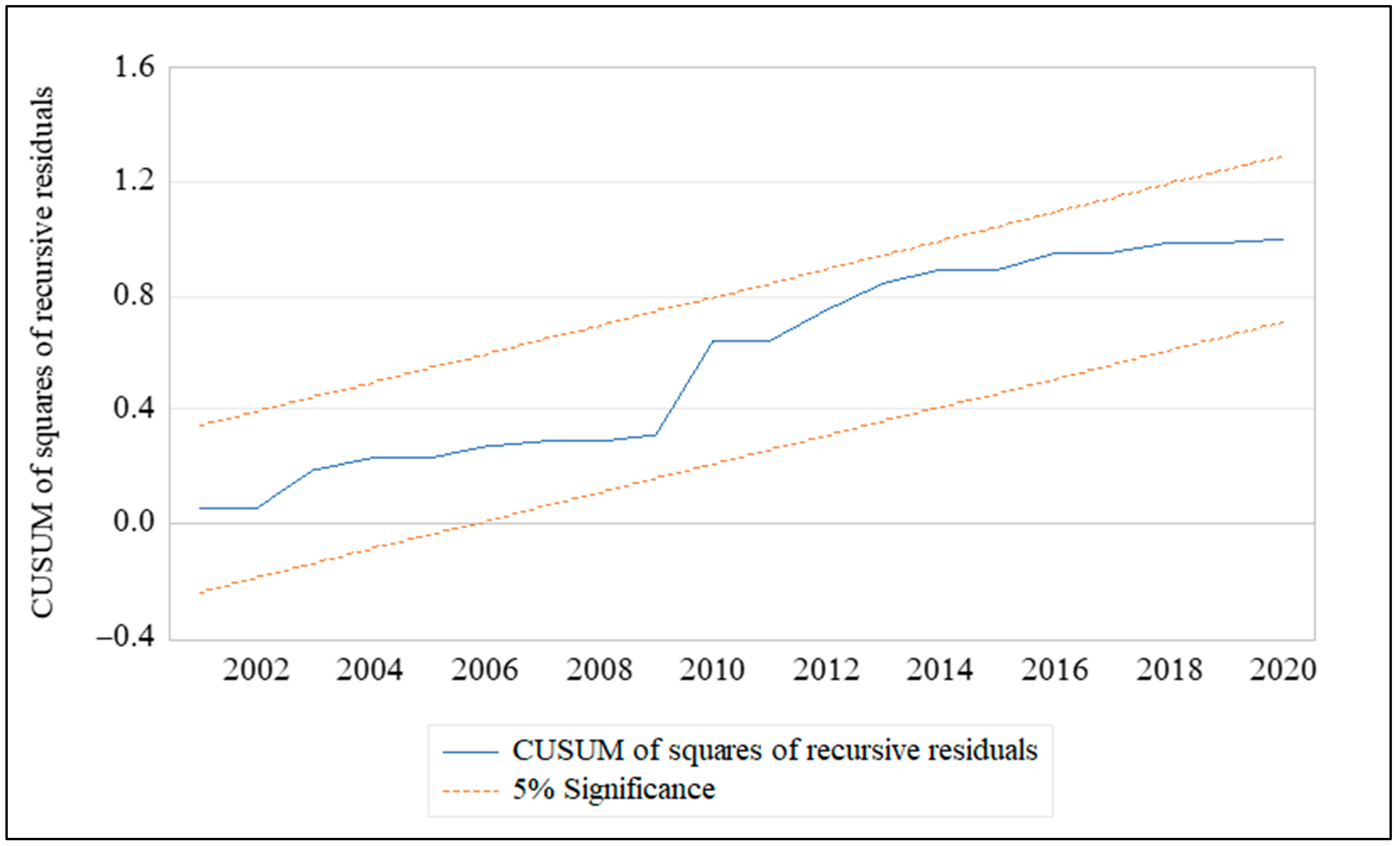
Figure 4.
Dynamic Multiplier of the response of CO2 emissions per capita. Notes: (1) The graph shows how a 1% shock to (LNFD_POS) and (LNFD_NEG) impact over time.
Figure 4.
Dynamic Multiplier of the response of CO2 emissions per capita. Notes: (1) The graph shows how a 1% shock to (LNFD_POS) and (LNFD_NEG) impact over time.

Figure 5.
Quantile estimates of the speed of adjustment with its 95% CI. Notes: (1) 95% confidence interval (CI) is the solid red line without the triangle marker. (2) Speed of adjustment refers to the coefficient on the error correction term.
Figure 5.
Quantile estimates of the speed of adjustment with its 95% CI. Notes: (1) 95% confidence interval (CI) is the solid red line without the triangle marker. (2) Speed of adjustment refers to the coefficient on the error correction term.
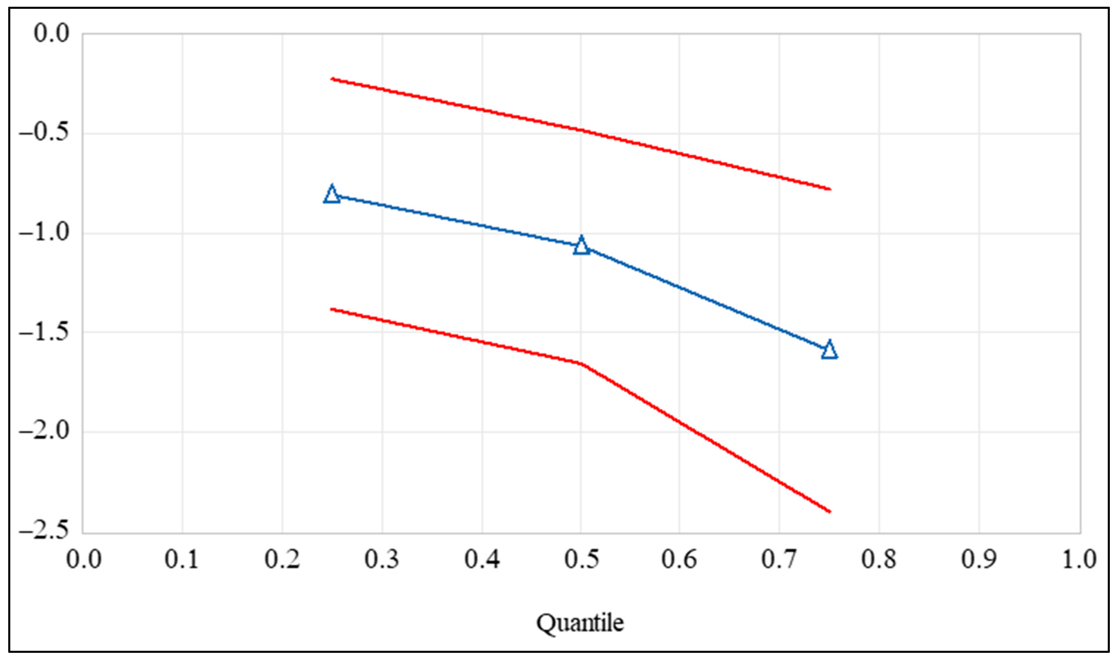
Figure 6.
Quantile estimates of the positive partial cumulative sums with their 95% CI. Notes: (1) 95% confidence intervals (CI) are the solid red lines without the marker. (2) , , and .
Figure 6.
Quantile estimates of the positive partial cumulative sums with their 95% CI. Notes: (1) 95% confidence intervals (CI) are the solid red lines without the marker. (2) , , and .
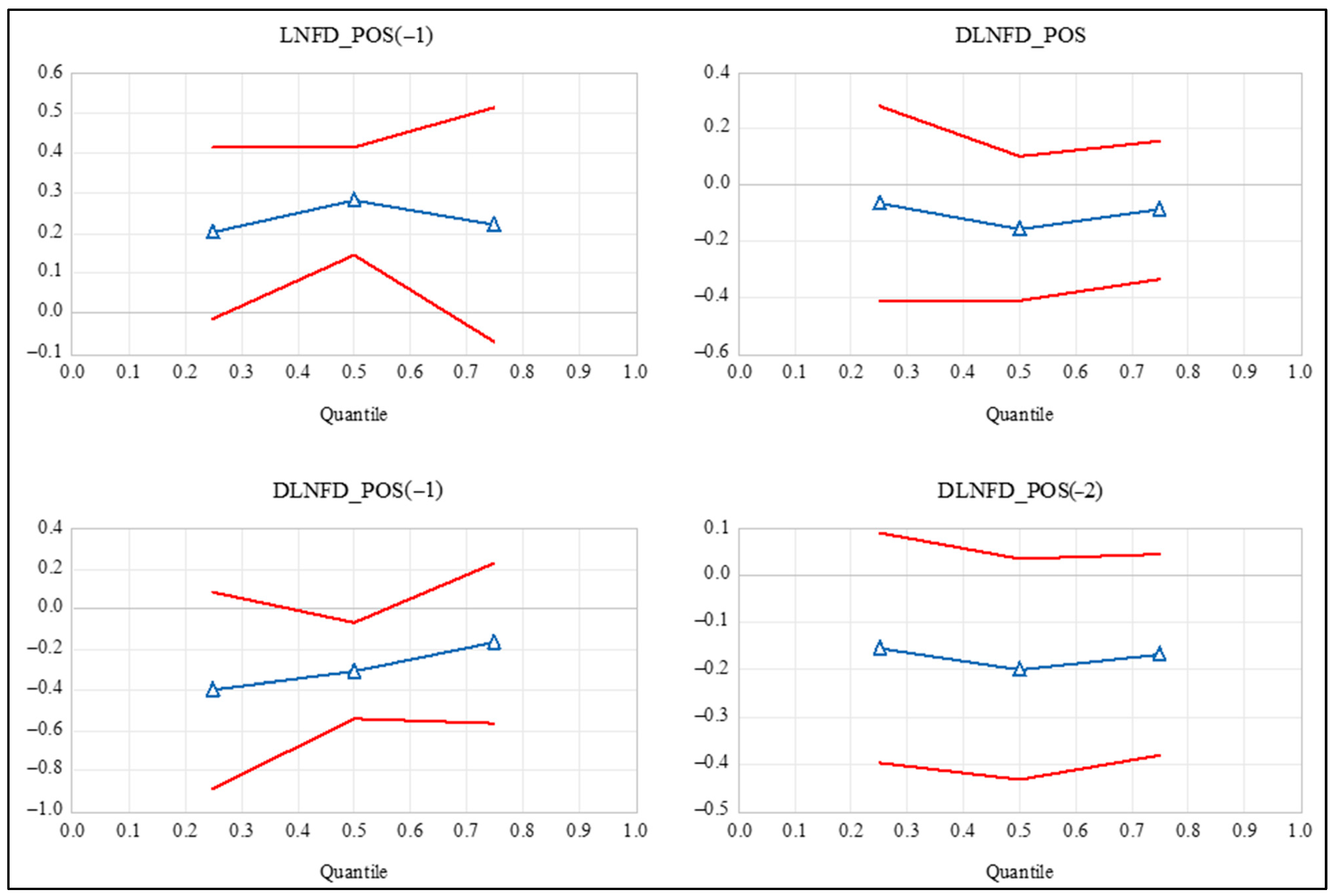
Figure 7.
Quantile estimates of the negative partial cumulative sums with their 95% CI. Notes: (1) 95% confidence intervals (CI) are the solid red lines without the triangle marker. (2) , and .
Figure 7.
Quantile estimates of the negative partial cumulative sums with their 95% CI. Notes: (1) 95% confidence intervals (CI) are the solid red lines without the triangle marker. (2) , and .

Table 1.
Unit Root Results.
| Variable | C.V. at 1% | Test Statistic |
|---|---|---|
| −3.61 | 0.03 | |
| −3.61 | −8.23 *** | |
| −3.61 | 0.24 | |
| −3.61 | −4.81 *** | |
| −3.62 | 0.20 | |
| −3.62 | −5.08 *** | |
| −3.57 | −2.03 | |
| −3.59 | −3.99 *** | |
| −4.21 | −0.13 | |
| −4.21 | −6.90 *** | |
| −3.54 | 0.22 | |
| −3.54 | −6.96 *** |
Notes: (1) *** indicates statistical significance at the 1% level. (2) The null hypothesis of the ADF test is that the series contains a unit root. (3) For , both trend and intercept were included. For all other variables, only the intercept was included. (4) C.V. refers to critical value.
Table 2.
NARDL Bounds Test.
| F-test, degrees of freedom = 1, 32 | |||
| F-test statistic | 9.82 *** | ||
| Significance Level | I(0) critical values | I(1) critical values | |
| 10% | 2.26 | 3.35 | |
| 5% | 2.62 | 3.79 | |
| 1% | 3.41 | 4.68 | |
| t-test, degrees of freedom = 36 | |||
| t-test statistic | −7.16 *** | ||
| Significance Level | I(0) critical values | I(1) critical values | |
| 10% | −2.57 | −3.86 | |
| 5% | −2.86 | −4.19 | |
| 1% | −3.43 | −4.79 | |
Notes: (1) *** indicates statistical significance at the 1% level. (2) F-test rejects the null hypothesis of no level relationship at 1% level as F-test statistic > F-test I(1) 1% critical value (9.82 > 4.68). (3) t-test rejects the null hypothesis of no level relationship at 1% level as t-test statistic < t-test I(1) 1% critical value (−7.16 > −4.79).
Table 3.
NARDL Bounds Test Diagnostics.
| Test | D.F. | Test Statistic | C.V. at 5% |
|---|---|---|---|
| Jarque–Bera Normality, χ2-test | 2 | 0.92 | 5.99 |
| Breusch–Godfrey Serial Correlation LM, F-test | (2, 18) | 2.72 | 3.56 |
| Breusch–Pagan–Heteroskedasticity, F-test | (16, 20) | 1.43 | 2.18 |
| Ramsey RESET, F-test | (1, 19) | 1.54 | 4.38 |
Notes: (1) The null hypotheses of none of the tests are rejected at the 5% level of statistical significance or less. (2) The null hypothesis of the Jarque–Berra test is that the data are normally distributed. (3) The null hypothesis of the Breusch–Godfrey Serial Correlation Lagrange Multiplier (LM) test is the absence of serial correlation. (4) The null hypothesis of the Breusch–Pagan–Godfrey test is homoskedasticity. (5) The null hypothesis of the Ramsey RESET test is that the NARDL model is not misspecified in the first order wherein the powers of the fitted values of the dependent variable would have explanatory power. (6) D.F. refers to degrees of freedom, and except for the Jarque–Bera Normality χ2-test, the first number in brackets is the D.F of the numerator and the second number is the D.F. of the denominator of the respective test. (7) C.V. refers to critical value.
Table 4.
NARDL Long-Run and Short-Run Equations.
| Variable | Coefficient | Standard Error |
|---|---|---|
| Long-Run Equation | ||
| 0.17 *** | 0.04 | |
| 0.12 | 0.11 | |
| 0.81 *** | 0.04 | |
| −0.23 ** | 0.09 | |
| −0.02 | 0.03 | |
| Short-Run Equation | ||
| −0.07 | 0.05 | |
| −0.29 *** | 0.06 | |
| −0.12 | 0.06 | |
| 0.11 | 0.07 | |
| 0.28 *** | 0.08 | |
| 0.30 *** | 0.10 | |
| 0.77 *** | 0.08 | |
| −0.36 | 0.34 | |
| 0.85 | 0.41 | |
| 1.99 *** | 0.52 | |
| −1.34 *** | 0.15 | |
| Wald χ2-test of asymmetry: D.F.= 1with C.V. at 1% = 8.10 and C.V.at 5% = 4.35 | ||
| Long-run χ2-test Statistic | 5.39 ** | |
| Short-run χ2-test | 10.75 *** | |
| Adjusted R-squared | 0.80 | |
| Akaike information Criterion | −4.85 | |
| Number of observations | 37 | |
| NARDL Model | (1, 3, 3, 1, 3, 0) | |
Note: (1) *** and ** indicate statistical significance at the 1% and 5% level, respectively. (2) D.F refers to degrees of freedom. (3) C.V. refers to critical value.
Table 5.
Quantile Slope Equality and Symmetric Quantiles Wald Tests.
| Coefficient(s) on | χ2--Test Statistic | D.F. | p-Value |
|---|---|---|---|
| Quantile Slope Equality | |||
| Error Correction Term | 3.83 | 2 | 0.203 |
| Positive Partial Cumulative Sums | 1.85 | 8 | 0.985 |
| Negative Partial Cumulative Sums | 4.05 | 8 | 0.852 |
| Symmetric Quantiles | |||
| Error Correction Term | 0.27 | 1 | 0.599 |
| Positive Partial Cumulative Sums | 1.53 | 4 | 0.822 |
| Negative Partial Cumulative Sums | 0.97 | 4 | 0.914 |
Notes: (1) Positive Partial Cumulative sums are , , , and (2) Negative Partial Cumulative Sums are , , , and . (3) D.F. refers to degrees of freedom and p-value to the probability value of the test statistic.
Disclaimer/Publisher’s Note: The statements, opinions and data contained in all publications are solely those of the individual author(s) and contributor(s) and not of MDPI and/or the editor(s). MDPI and/or the editor(s) disclaim responsibility for any injury to people or property resulting from any ideas, methods, instructions or products referred to in the content. |
© 2023 by the authors. Licensee MDPI, Basel, Switzerland. This article is an open access article distributed under the terms and conditions of the Creative Commons Attribution (CC BY) license (https://creativecommons.org/licenses/by/4.0/).
Share and Cite
MDPI and ACS Style
Das, A.; Brown, L.; McFarlane, A. Asymmetric Effects of Financial Development on CO2 Emissions in Bangladesh. J. Risk Financial Manag. 2023, 16, 269. https://doi.org/10.3390/jrfm16050269
AMA Style
Das A, Brown L, McFarlane A. Asymmetric Effects of Financial Development on CO2 Emissions in Bangladesh. Journal of Risk and Financial Management. 2023; 16(5):269. https://doi.org/10.3390/jrfm16050269
Chicago/Turabian StyleDas, Anupam, Leanora Brown, and Adian McFarlane. 2023. "Asymmetric Effects of Financial Development on CO2 Emissions in Bangladesh" Journal of Risk and Financial Management 16, no. 5: 269. https://doi.org/10.3390/jrfm16050269