
A Cautionary Note on the Use of Accounting Semi-Identity-Based Models †


Departamento de Economía, Contabilidad y Finanzas, Facultad de Ciencias Empresariales, Universidad Politécnica de Cartagena, 30201 Cartagena, Spain
†
This paper is an extended version of the work Presented at the XVIII 2018 Conference, Lisboa, Portugal, 20–21 September 2018. The 7th Spring Multinational Finance Society Conference, MSF-2019, Crete, Greece, 19–21 April 2019, and a sequel of the 2007 article: The problem of estimating models using ac-counting semi identities. IVIE Working paper.
J. Risk Financial Manag. 2023, 16(9), 389; https://doi.org/10.3390/jrfm16090389
Submission received: 10 July 2023
/
Revised: 21 August 2023
/
Accepted: 24 August 2023
/
Published: 30 August 2023
Abstract
:This study employs a Monte Carlo simulation to see whether accounting identity problems are present in the Fazzari, Hubbard, and Petersen model (1988). The Monte Carlo simulation generates 50,000 random cash flows, Tobin’s Q, and error term variables, which shape an investment variable that is dependent on them. Cash flows and investments are linked by a partial accounting identity, also known as an accounting semi-identity (ASI). An accounting identity is, for example, an equality between the left and right sides of a balance sheet. An ASI is not a complete one since one or more components of the accounting identity are missing. The estimated coefficients of an ASI do not represent reality, according to the OLS estimations. The regression tells us less about causality the closer the data are to the accounting identity. This is the first time that the biases of OLS estimations in an ASI-based model have been demonstrated.
“Mistakes and errors are the discipline through which we advance.”William Ellery Channing
“Keynes’s critique of the classical economists was that they had failed to grasp how everything changes when you allow for the fact that output may be demand-constrained. They mistook accounting identities for causal relationships”.
“It is important for those who want to achieve certainty in their research, knowing how to doubt in time”.Aristotle
“Advice to Scott: Avoid Accounting Identities at ALL Costs”.
1. Introduction
Financial management literature typically assumes that the cash flow a company generates during a year strongly influences the investments that the company makes during the same period. Fazzari et al. (1988) related these two accounting variables in a linear regression model, calling the coefficient of the explanatory variable investment-cash flow sensitivity. Companies with severe information asymmetry problems find that external financing is either too expensive or unavailable (Farooq et al. 2022). Fazzari et al. (1988) argued that the higher the explanatory variable coefficient, the more company investments depend on company cash flow to finance them. So, higher coefficients should correspond to companies with more severe information asymmetry and, therefore, greater financing restrictions.
Since then, many studies using this model have shown results that strongly contradict the hypothesis that the more financially constrained a company is, the more sensitive its investment–cash flow relation. Brown and Petersen (2009) and Chen and Chen (2012) are examples. The best-known studies questioning the implementation of this model are the two articles by Kaplan and Zingales (1997, 2000), who found higher estimated coefficients for the cash flows of companies with fewer financial constraints. Two samples—one comprising US enterprises and the other Canadian firms—were used by Cleary (1999), who surprisingly discovered that while the Canadian sample supports the Kaplan and Zingales (1997, 2000) results, the US sample supports the Fazzari et al. (1988) model (FHP model hereafter). Bhabra et al. (2018) showed that the investment–cash flow sensitivity of companies that are not financially limited is, in fact, higher than that of firms that are.
Chen and Chen (2012) found that investment–cash flow sensitivity had drastically declined over the past 40 years and had all but vanished in the latter years of their sample. According to their results, this trend cannot be accounted for by a decline in the significance of cash flow as a source of financing, nor can it be explained by a number of factors the academic literature considers decisive. This evidence is similar to that of Machokoto et al. (2021), whose work can be seen as a sequel to Chen and Chen’s (2012). They found that investment–cash flow sensitivity had decreased, even during the global financial crisis starting in 2008, when rationale dictates the opposite should occur. They also found that the factors mentioned in the literature cannot account for the decline in investment–cash flow sensitivity. So far, the reason why the model estimation does not work has not been clarified.
This issue is at the cutting edge, as many works continue using the FHP (1988) model and continue to obtain inconclusive and opposing findings. In the first 2 years and 5 months of this decade, at least 24 articles published in top journals used this model, and no less than 12 of them in journals from the first decile of JCR’s most recent database (2022). Some of these articles include comments on the difficulty of explaining some of their results. The solutions usually involve including varied factors, which distort the regressions’ associated results (and the underlying ASI, as we shall see in subsequent sections). Among the works with contradictory results, we have Guariglia (2008); Carpenter and Guariglia (2008); Chen et al. (2016); Lewellen and Lewellen (2016); Ağca and Mozumdar (2017); and Kashefi-Pour et al. (2020), who found increasing investment–cash flow sensitivity, whereas others (Chen and Chen 2012 and Moshirian et al. 2017) confirmed a decreasing linkage. This has led some authors to express their skepticism. Gautam and Vaidya (2018) concluded that firm-specific financial constraints could not be associated with investment–cash flow sensitivity, Kabbach-de-Castro et al. (2022a) stated that “prior research is not conclusive whether information asymmetries or managerial discretion are the cause of observed investment–cash flow sensitivity”. Adu-Ameyaw et al. (2022) pointed out that the literature on the investment–cash flow linkage is inconclusive, and Wang (2022) reckoned that the strange results of empirical evidence concerning the FHP (1988) model “remain a puzzle to be explained”. The shadow of doubt growing among authors who use accounting semi-identity models has led some to include cautionary comments when estimating partial accounting identities (see, for example, Maskay et al. 2018; Minenna 2022). Trying to elucidate why the researcher can obtain strange and counterintuitive results when using the FHP (1988) model is of maximum interest and is the aim of this paper.
In this paper, I propose that the problem is caused by the fact that the FHP (1988) model is a partial accounting identity or accounting semi-identity (ASI hereafter). The concept of ASI is rarely seen in academic literature. Apart from Sanchez-Vidal (2007), it has only been referred to in Lambelet and Schiltknecht (1970) and Mattei (1976), who mentioned the concept to introduce some semi-identities in their estimations. As authors are becoming increasingly aware of this problem, it has been discussed recently in the works mentioned above by Maskay et al. (2018) and Minenna (2022) and in Christodoulou and Mcleay (2019), who called it a “Double Entry Constraint”. This fact may create a problem and distort results, as I demonstrate in Sanchez-Vidal (2007). An ASI is an accounting identity but not a complete one since one or more components of the accounting identity are missing. The FHP (1988) model is an ASI because some components of the accounting identity contribute to both the independent and dependent variables. Since the identity must be satisfied mathematically, the estimated regression coefficients (alleged investment–cash flow sensitivities, in this case) do not have the same meaning as in an analysis of a causal relation in a standard regression. The research method of this article employs Monte Carlo simulations, as it has the advantage of retaining complete control of the relations the researcher is interested in analyzing. This approach is the first to demonstrate that working with ASIs may constitute a serious problem. The following is a breakdown of the paper’s structure. The next section contains a review of the literature. Section 3 describes the Materials and Methods. Section 4 reports the results, Section 5 includes the discussion, and Section 6 concludes the paper and gives indications of future research.
2. Literature Review
Accounting identities have been previously used in academic research because of their properties (see, for example, Wirkierman 2023), which help, for example, to deduce unknown components of it (see De Mesnard 2023). The problem comes when the accounting identity is used as an equation to estimate relations through linear regressions. The critique about the use of ASI could be considered an extension of the accounting identity critique. Criticism about the use of accounting identities in the economics, finance, and accounting research literature has generated academic discussion for at least the last six decades, raising increased doubts that the use of accounting identities is effective in models to describe causal relations.
The first authors to note the problem did not usually comprehend the full implications of the accounting identity problem, resulting in a somewhat restrained critique. Intriligator (1978), for one, realized that the accounting identity could make a difference, noting merely that the estimation of a production function that is an accounting identity would produce biased estimates. Similarly, McCallum (1995) argued that a bias problem might arise if the disturbance term in an accounting identity were correlated with the regressor. Giles and Williams (2000), writing about models that relate exports to economic growth, said, “Some of the results may involve a spurious correlation due to exports themselves being part of national product”, leading to what they call “an accounting identity effect” (p. 265). Currie (1976) thought that in the estimation of a model that is based upon the balance of payments identity or the budget deficit identity, the problem is merely one of causality. Many authors who advocate a causality problem have tried to resolve the question by applying the Granger causality test, like Marin (1992).
The fiercest accounting identity critique to date is related to the discussion of the usefulness of the Cobb–Douglas (C-D) production function, which is a well-known accounting identity. Since the mid-20th century, many researchers have observed that using accounting identities could create serious estimation problems. The issue merited mention in Herbert Simon’s (1979) Nobel Lecture. There, he observed that one cannot take previous evidence found when estimating the C-D function as a support of the use of that function “for identical results can readily be produced by mistakenly fitting a C-D function to data that were in fact generated by a linear accounting identity (value of goods equals labor cost plus capital cost)” (p. 348).
As Dorman (2007) noted, talking about a model that comes from an accounting identity, “this means that it is wrong to appeal to the identity as evidence for the model, or to claim that the purpose of the model is to ‘explain’ the identity. There is nothing to be explained” (p. 55). Felipe et al. (2008) argued that “[the use of variables that are] related definitionally through an accounting identity… prevents meaningful econometric estimates of the production technology”. The debate about the accounting identity problem is as alive as ever at this point in time (see Felipe and McCombie 2020; Felipe et al. 2021).
The impossibility of estimating causal relations when using a full accounting identity has been demonstrated by several authors. Fisher (1971) resorted to simulation analysis to shed light on why the aggregate C-D production function works when, in theory, it should not. Fisher et al. (1977) also resorted to simulations and argued that “The aggregated simulated data gave plausible estimates of the value of the ‘aggregate elasticity of substitution’, which in the simulations did not exist”. In other words, “the elasticity of substitution in these production functions is an ‘estimate’ of nothing” (p. 442). Shaikh (1974) simulated data with no economic meaning that yielded good explanatory results about the C-D production function due only to the accounting identity.
2.1. The FHP Model Is an ASI
In the 2007 article, “The Problem of Estimating Causal Relations by Regressing Accounting (Semi) Identities”, I elucidated why many empirical estimations of the FHP (1988) model frequently give unexpected outcomes. The investment–cash flow sensitivity model is an ASI because both the dependent and independent variables are “simply left-hand and right-hand side long-term components of the balance sheet of a company” (p. 4). The Sanchez-Vidal (2007) demonstration is reproduced in Figure 1.
The complete accounting identity is given by the expression:
I will call all the elements in the parentheses the “rest”, as in Sanchez-Vidal (2007).
If the researcher applies OLS to Equation (1) as if it were a causal relation, thus adding an error term, the elements performing in the estimation in matrix formulation:
would become these specific values for the design matrix:
As the OLS attempts to minimize the sum of the squares of the differences between the investments and those predicted by the linear function, the smallest difference matrix will result in the following estimates: . These estimated meet Equation (1) perfectly from an arithmetic point of view, and thus, the R2 will be 100%. The OLS will produce these results because its goal is also met: these coefficients constitute the best fit in the least-squares sense at the same time. Section 3 explains how a simulated database, including all the variables in the accounting identity, is created. Meanwhile, we can advance the results of the regression with the simulated database for the complete accounting identity: in Table 1.
As I have commented above, it is not surprising that the results yield estimated coefficients of 0 for , 1 for and , and an R2 of 100%. This evidence is consistent with the reasoning by Farris et al. (1989), who argued that “coefficients should be unity when estimating a perfect accounting identity, because any other result would simply indicate errors in the data”. It is easy to deduce that when the “rest” is very small in absolute value compared to that of the other independent and dependent variables, and we are, thus, modelling an ASI that is very near the accounting identity it comes from, the results will be very similar: the coefficient of the cash flows will tend to 1 and the R2 to 100%. Felipe and McCombie (2001) commented on the good fit of the C-D production function estimation and pointed out that: “All that the data are actually reflecting is an underlying accounting identity and, consequently, it is not surprising that the coefficients are usually well determined and the correlation coefficient not far from unity” (p. 1221).
2.2. Hypotheses
In Sanchez-Vidal (2007), I explained that the investment–cash flow sensitivity model as proposed by Fazzari et al. (1988) consists simply of regressing the accounting identity (expression (1), but without the “rest”:
Due to the use of an ASI, the results of the FHP model could be influenced by that “rest”. The coefficient of an OLS regression will adjust itself to satisfy the identity since it “will have to offset this absence” (p. 6). In this regard, Farris et al. (1989) stated that when there is a missing component in an accounting identity-based model, the coefficients of the remaining identity components will adapt to meet the identity. If, for example, both investments and cash flows are positive and the “rest” is positive (negative), the coefficient will be higher (lower) than unity because of the identity.1 The example in Sanchez-Vidal (2007) of a negative “rest” case is as follows:
“Consider a company that has invested $5 million in a year, has generated $7 million of cash flows, and “the rest” is equal to −$2 million. To satisfy the complete identity, estimating expression (1) for this company would lead to these results: 5 = 0 + 1 × 7 + 1 × −2.
But, as the −2 is missing in Equation (1), the coefficient of the cash flow variable will have to offset this absence: 5 = 0.714 × 7, that is, a value lower than 1”.
In arithmetic terms, if most of the companies tend to show similar values of X1 (cash flows) and Y (investments) to those of the example, the coefficient will be positive, or, in other words, the coefficient of cash flows will be determined by the value of the “rest”. As a result, the first hypothesis to investigate is:
Hypotheses 1 (H1).
The FHP (1988) model’s outcomes may be influenced by the “rest” of the complete accounting identity, i.e., the sum of the accounting identity variables not included in the model.
I have commented that similar values of the variables will probably help arithmetics to impose over causality and bias the “true” value of the cash flow coefficient. This will probably be the case when, for example, investments and cash flows tend to be positive, and cash flows are higher than investments in many of the observations. A more extreme case occurs when the relation between the cash flow variable and the “rest” is very stable across observations.
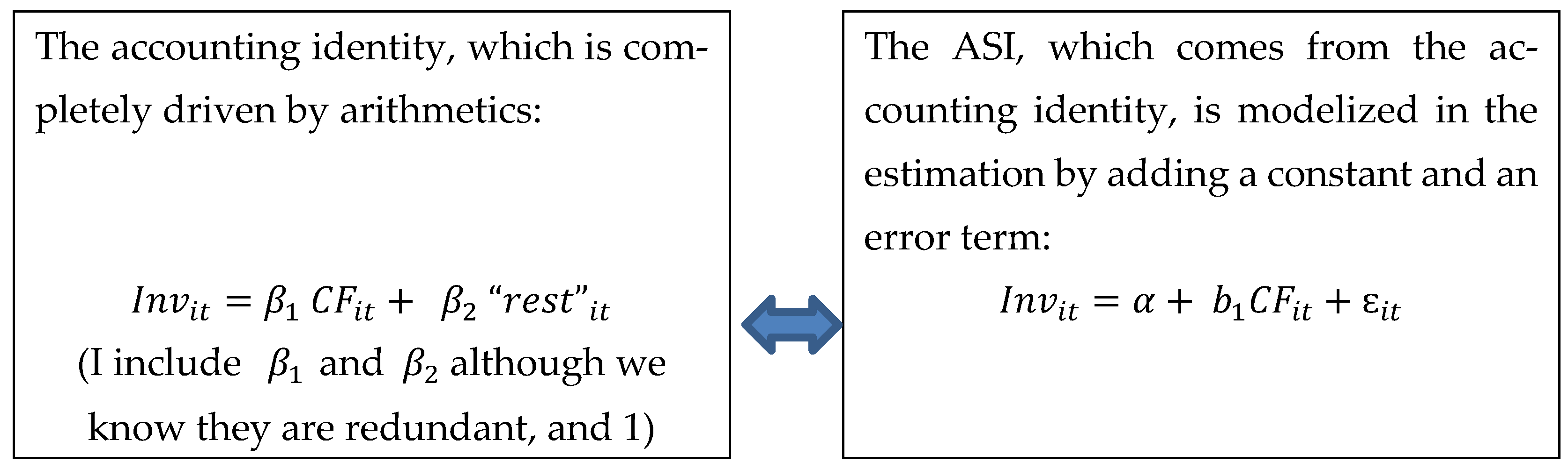
First, let us recall that the relation in the FHP (1988) model between the accounting identity and the ASI coming from it can be summarized in Figure 2 as follows:
So, the link between arithmetics and the OLS formulation is defined by this equality: .
From an econometric point of view, Equation (2) (ASI) is Equation (1) (accounting identity) with an omitted component. We all know that in a standard estimation with an omitted variable, there can be a specification bias if this omitted variable is correlated with the included variable (see Gujarati and Porter 2013). The mathematical expectation of the coefficient of the included explanatory variable b1 is: Let us consider the case where the value of the “rest” is approximately 50% of the cash flow variable. At this point, it is easy to deduce that there will be a bias, not only because the cash flows and the “rest” are obviously correlated due to the accounting identity, but also because the relation between and is somewhat fixed, as: , with = 0.5 in this case. Let us imagine that in most companies, the ratio between these two components of the accounting identity meets this condition. This uniformity makes the ratio between the “rest” and cash flow very stable, and as and , then: . This leads to Hypothesis 2.
Hypotheses 2 (H2).
If the ratio between the “rest” and the cash flow variable tends to a certain value in the FHP (1988) model: Ө, the regression will yield an estimated coefficient which will tend to have a value = (1 + Ө).
In this case, in our accounting identity, then from the ASI and from the accounting identity will coincide, as the OLS will tend to produce an estimated of (1 + Ө). This leads to Hypothesis 3.
Hypotheses 3 (H3).
The more homogenous the ratio between the cash flow variable and the “rest” is, the less space there is for a causal relation, and so the estimated coefficient will tend to be statistically different from its true value, 0, and the R2→100%.
As in Shaikh (1974), I employed a Monte Carlo simulation to show that using an ASI can also produce meaningless results. The direct relationship between investments and cash flows is impossible to measure directly in real life due to the problem discussed in this article, and for that reason, a simulation method is well suited to the study of this phenomenon. We can draw conclusions about the problems of a model coming from an ASI by using simulated relationships between variables in a model. To the best of my knowledge, this is the first time that the use of OLS has been shown to be useless for estimating the FHP (1988) model.
3. Materials and Methods
It will be impossible to infer a causal relationship in a regression using real data if the ASI problem implications are valid. The rationale for this is that any significant coefficient found using an OLS regression could be either the product of an arithmetic illusion, the evidence of a causal relationship, or both. As these two “forces” may be mixed, the researcher will not be able to disentangle them when implementing linear regressions with real data.
3.1. Research Method: Monte Carlo Simulations
Motivated by these considerations, I used a Monte Carlo simulation to examine the implications of these arguments. For economists, data generated through computational techniques used to model a system are a relatively recent phenomenon and, although initiated only some decades ago, are becoming increasingly popular (see, for example, Wang 2023). The advantage of using Monte Carlo simulations is that the researcher can actually generate causal relations, defining and controlling them perfectly. Until now, no study has used a simulation to investigate the issue of ASI, even though some researchers have used it to address the challenge of a complete or full accounting identity (see Shaikh 1974).
3.2. Dataset
The simulation design consisted of randomly generating (using the normal distribution) 50,000 sets of error terms , with a mean of zero and a standard deviation of 0.1; 50,000 sets of a cash flow variable, , normally distributed with a mean of 0.25 and a standard deviation of 0.1; 50,000 sets of a randomly generated Tobin’s Q with a mean of 2.45 and a standard deviation of 0.2; and another 50,000 sets of error terms with a mean of zero and a standard deviation of 0.1. As in any Monte Carlo simulation, the choice of parameters is “necessarily rather arbitrary” (Carbone 1997). All of the parameters in this Monte Carlo simulation (investments, cash flows, and Q) had mean and standard deviations corresponding to the average values of the four subsamples of firms in Fazzari et al. (1988, pp. 22, 25). The cash flow and investment values may appear high, but the reader should keep in mind that the variables in Fazzari et al. (1988) are scaled by K, or the replacement cost of assets at the beginning of period t, namely, the value of fixed assets written down by their depreciation. In this example, CF had an average of 25%, a positive value, and was very probably associated with a positive average ROA in year t in an equivalent real company, which was a result in line with the expectations of an enterprise in a true economy. The mean of Tobin’s Q showed a value of 2.45. Taking into account that the denominator was again K and the numerator was total assets minus inventories, with the market value of equity substituted for its book value, this average value for a company probably indicated that financial investors overvalued it and/or the enterprise-inspired solid market confidence, mainly due to expected sound future performance and a good set of investment opportunities.
The Monte Carlo design was run with the statistical software Stata 13.0, and the computer code to reproduce the simulation is fully available along with this work.
3.3. Model
In the FHP (1988) model, the investments depend on cash flows, Tobin’s Q, and a constant:
Given that the researcher is attempting to mirror reality through simulations, I utilized this Monte Carlo method to simulate the various sources of uncertainty (inputs) that affect the investments under consideration. Then, given these possible values for the underlying inputs, I determined a representative simulated value of investments. The investments that each company undertakes depend on the internal funds the company has generated and a concrete value of Q. The following shows how the investment variable in the simulation will be affected by the randomly generated CF, Q, and error term for each company:2
The specific values chosen to create the investments variable give this variable a mean similar again to that of Fazzari et al. (1988). The result is that when the cash flows are increased by 10%, each company’s investment increases by 4.5%. I also forced investments to be dependent on the Q so that a one-unit increase in this variable results in a 3% rise in investments. The values of the CF, Q, and error term variable standard deviations were chosen to coincide with the standard deviations of the Fazzari et al. (1988) variables, too. The statistics that describe the simulated variables, “rest” included, are listed in Table 2. This Monte Carlo simulation will generate 50,000 alternative outcomes by sampling from a probability distribution for each of the independent variables ().3 The raison d’être of the error term is to represent all those factors that affect investments but are not explicitly taken into account (Gujarati and Porter 2013). An example is agency costs. Managers could have incentives to overinvest or underinvest due to other corporate governance considerations, as pointed out by, for example, the free cash flow theory (Jensen 1986).
4. Results
Table 3 serves to test Hypothesis 1. With this in mind, the model specification of the regressions in this table does not include the Q variable, as in Fazzari et al. (1988, p. 18, expression (20)). Estimates were made for the entire sample and subsamples of companies based on the sign of “the rest”. The findings of the first column (the whole-sample estimation) produced a coefficient for the cash flow variable (0.45) that accurately represents the real impact of this variable on investments. This result was not statistically different from the true 0.45. The constant is significant, probably borrowing part of the influence of the omitted Q variable.
The second and third columns show the regressions for the subsamples divided by negative and positive “rest”, respectively. Since the cash flow variable’s coefficients were statistically different from 0.45, they failed to be valid in either of the two subsamples. The coefficients were affected by the ASI and the sign of “the rest”, confirming Hypothesis 1. The positive “rest” subsample’s coefficient was statistically higher and different from the negative “rest” subsample’s. The negative “rest” subsample’s coefficient was higher than the overall sample’s. A lower coefficient might have been a more reasonable finding, but as discussed in note 1, the existence of the constant introduces interferences. When employing multiple accounting identity specifications with arguments missing, Felipe and McCombie (2009) stated that this omission “may, of course, lead to biases on the coefficients of the remaining variables, and sometimes in an unpredictable way” (p. 152). The volatility of the alleged “investment–cash flow sensitivity” value could explain the results of Kabbach-de-Castro et al. (2022b), who observed that this sensitivity varies “across firms and economies” in their sample. The results are also an early confirmation of Hypothesis 3 because when dividing by signs of the “rest”, the resulting subsamples were more homogeneous, and this implies more biased coefficients and better fits, which were confirmed by the coefficients and the increasing R2. When estimating the FHP (1988) model, Peters and Taylor (2017) found R2, which, to no surprise, increase when subsampling by more homogeneous subsets.
In regression 4 of Table 3, I created a multiplicative dummy variable that equals the value of cash flows when “the rest” is positive and 0 otherwise. I, therefore, have definitive proof of Hypothesis 1. This enabled a joint estimation of both subsamples while avoiding the constant’s troublesome, unpredictable behavior. For this multiplicative dummy, the results in the last column yielded a positive and significant coefficient. The value of its coefficient (0.67) was the measure of the error that is the focus of my argument and a further confirmation of Hypothesis 1. This cannot be explained by a conventional causal relation scheme and should dispel any objection about the influence of the ASI. Furthermore, this dummy is the most significant of all the variables in the four regressions.
Table 4 serves to explore Hypotheses 2 and 3. In this table, I explore different degrees of homogeneity in the relation between and (cash flows and “the rest”) for Equation (3). Column I estimates Equation (3) with the example of a very stable ratio (=0.5 ± 1%) between the “rest” and cash flows I commented on in Section 2. When the ratio is nearly a constant, the results showed that homogeneity matters, as the coefficient for the cash flows is useless and completely dependent on the ratio .
The results confirm Hypothesis 2 as arithmetics crowd out the causal relation completely. Tobin’s Q variable was non-significant, when it should have been. The value of the coefficient of the cash flows which tends to (1+ Ө) confirms the prediction and lies quite far from its true value of 0.45. This is the result of working with accounting identities and ASIs, which pose a phenomenal challenge because, as Minenna (2022) stated, “the closer the data are to an accounting identity, the less information on causal relation can be inferred from econometric techniques”. The results also confirm Hypothesis 3, as homogeneity in the relation between and : cash flows and the “rest”, (which is the same as imposing a homogeneous relationship between investments and cash flows), resulted in the ASI approaching the accounting identity and causing a very high fit for the regression, although the number of observations is remarkably low.
In Column II, the ratio was allowed to vary between 0 and 1. The cash flow coefficient deviated from the value that the ratio imposes, although it was not yet the true coefficient. The Q variable was significant but far from its true value; the constant was also significant, and the adjusted-R2 fell to the 77% level. In Column III, the ratio was allowed to vary between −5 and 5. The coefficients of the cash flows and the Q variable were very close and not statistically different from the true values. Finally, in Column IV, with no restrictions on the relation between and (cash flows and “rest”), the coefficient for cash flows was correct. As Column IV of Table 4 is equivalent to the first estimation of Table 3 but included the Q variable, the constant now loses significance with the appearance of Q, or to put it differently, the constant was previously significant because it was most likely borrowing some of the influence from the omitted Q variable.
The estimated coefficient for this variable started to become “correct” in Column III, confirming that when the restriction the ratio imposes is high (as it happened in the first two columns), even ‘outside’ variables are affected. The non-restricted estimation of Column IV shows all of the genuine relationships between investments and cash flows, as well as Tobin’s Q. The extraordinary better-fits when the subsamples are more homogeneous (Columns I and II) do not correspond to reality. Felipe and Holz’s (2001) evidence of an increased R2 is similar to mine. When they constrained simulations to be linked through the accounting identity, they noticed that the R2 rises dramatically when estimating the production function. The conclusion is that the force of arithmetic entirely masks the causal relation. Causality is, in these examples, gone with the wind.
5. Discussion
Results of the previous section, taking into account the accounting identity, give an explanation of the strange results of the Fazzari et al. (1988) model to date. According to one previous work of mine, Sanchez-Vidal (2007), the ASI problem is probably to blame for the counterintuitive results by Kaplan and Zingales (1997) when they used the FHP (1988) model. Less constrained enterprises are more likely to experience larger investment–cash flow sensitivity since it is easier for them to add long-term debt, increasing the value of “the rest” and resulting in higher estimated coefficients for the cash flow variable, contrary to FHP (1988) model predictions. To check the validity of this assessment, I used a real database to see how important long-term debt as a component of the “rest” variable is.4 When computing a contingency table by comparing the distribution of the negative/positive sign of the “rest” subsamples and the negative/positive variation in long-term debt subsamples, the χ2 is significant at the 1% level. So, increasing/reducing long-term debt in a certain year is significantly related to a positive/negative “rest” and, for example, the fact that the long-term debt is positive/negative leads to a five-times greater probability of having a positive/negative “rest”, respectively, than the other way around.
6. Conclusions
By classifying enterprises as more or less financially constrained, the FHP (1988) model claims to be useful. The authors proposed regressing a company’s investments on its cash flow. Due to financing constraints, a high and significant coefficient should indicate that a company is heavily reliant on internally generated money to grow. Researchers have attempted to estimate the FHP (1988) model since it was developed, but many have reached strange and improbable conclusions. Kaplan and Zingales’s (1997, 2000) studies are the most important attempts to explain these abnormalities. They came to the end of their investigation without knowing why the model failed.
This article contended that the reason the FHP (1988) model does not work is because it is based on an ASI. An ASI is an accounting identity that is missing some components. The use of accounting identity-based models has been met with widespread criticism, most of which is focused on the literature about the estimation of the C-D production function. Simulations have been used by some authors to show that the conclusions obtained by estimating the C-D production function are incorrect.
In Sanchez-Vidal (2007), I explained what happens when an ASI is estimated. The predicted coefficients will most likely compensate for the absence of “the rest” or the sum of the accounting identity’s missing components. Since the variables cannot fluctuate freely, and the identity represents a tight restriction, the ASI problem will most likely become more severe as the ASI becomes closer to the full accounting identity, producing considerable biases in the coefficients and raising the R2. This may happen either when the omitted part of the accounting identity is relatively small or when the relation between the dependent variable and the included independent variable is similar across observations.
To test this problem, a Monte Carlo simulation is useful because it creates a synthetic relation between a company’s investments and its cash flows. Because of the problems with ASI models that this article has demonstrated, this relationship is otherwise unobservable in real life. In the Monte Carlo simulation, enterprises’ investments are influenced by cash flows. Because investments and cash flows are linked through the accounting identity, I also computed “the rest”. Then, in subsamples defined by the sign of “the rest”, I estimated the regression of investments on cash flows. The findings confirmed the first hypothesis that “the rest” influences the calculated results of the coefficients, whose values do not correspond to reality. The results also confirmed that the more homogeneous the relation between variables, the closer the ASI is to the full accounting identity. Thus, the R2 is higher, and the estimated coefficients and their significance are more distorted (Hypotheses 2 and 3).
I deduced from the Monte Carlo simulation that the OLS results do not correspond to a causal relationship and that the ASI problem is to blame for the biased coefficients, false negatives, incorrect R2, and erroneous significances in general. This work throws cold water on some of the literature on the FHP (1988) model, and it is a warning to seafarers of the peril of using OLS when estimating models based on ASIs. Researchers will most likely arrive at conclusions that have little to do with the underlying relationships that exist in reality. This problem is a consequence, as Shaikh (1974) put it, of the laws of arithmetic rather than the laws of causality.
Occam’s razor principle asserts that the simplest solution is usually the correct one.5 I concluded that the FHP (1988) model estimation results by Kaplan and Zingales (1997, 2000) are probably due to the model being an ASI. Companies that are less financially constrained but show an unexpectedly high cash flow coefficient will almost certainly witness increases in long-term debt (more likely in less constrained enterprises). This implies a higher “rest”, which, in turn, will bias the cash flow coefficient upward due to the ASI. This is the most straightforward explanation for what has happened with estimations of the FHP (1988) model so far. This is the first study to show that the Fazzari et al. (1988) model’s OLS estimation can produce biased results.
Future investigation should continue with this line of research and, for example, find a test in order to establish whether the results obtained using an ASI model with a concrete database to explore causal relations are valid or not. It could also be of the utmost interest to review the models in the areas of Economics, Finance, or Accounting, which are affected by the ASI problem. In addition, there is a need to open a research strand to find solutions to this problem, such as trying to break up the identity using a proxy for the dependent or independent variable, very related to the variable that is trying to replicate, but which makes the ASI problem vanish. In order to analyze how the investments of companies with different degrees of financial constraints react to cash flows, it could be useful to explore other research approaches (as Tettamanzi et al. 2023 pointed out), such as “experimental design …, case studies or interviews”.
Funding
This research received no external funding.
Data Availability Statement
The data presented in this study are openly available at: https://figshare.com/articles/dataset/FHP_Model_-_SAI/23112776 (accessed on 22 August 2023).
Acknowledgments
I would like to thank Francesco Fasano, José Antonio Martínez, Mari Luz Mate, Sven Steinkamp, the referees for help and suggestions and the conference participants at the 2018 AECA Conference and the 2019 Multinational Finance Society Conference for helpful comments.
Conflicts of Interest
The author declares no conflict of interest.
| 1 | I contended that this will also depend on the constant, as its magnitude, if positive or negative enough, can have an impact on the overall sum and modify the results. This may also happen when adding another variable, like the Q of the FHP (1988) model. In the end, it is a question of arithmetic, and all the addends should be taken into account. |
| 2 | Again, I resorted to arbitrariness to construct this relation (Carbone 1997). Nevertheless, this example of a simulated model is similar to that which can be found in any basic Handbook of Finance, for example, the Electric Scooter Project example in Brealey and Myers (2003, p. 263). |
| 3 | Replicability is the ability to independently arrive at non-identical but at least similar results when differences in sampling, research procedures, and data analysis methods may exist. The scientific method in economics requires replicability, and its execution varies greatly among research disciplines and fields of study (see Repko 2008). Since I used Stata to produce the data and wanted to make my simulation repeatable, both the syntax and the file are available at: https://figshare.com/articles/dataset/FHP_Model_-_SAI/23112776 (accessed on 22 August 2023). |
| 4 | Results not reported but available under request. |
| 5 | Occam’s Razor is Numquam ponenda est pluralitas sine necessitate (Plurality must never be posited without necessity) (Lombardi 1495). |
References
- Adu-Ameyaw, Emmanuel, Albert Danso, Moshfique Uddin, and Samuel Acheampong. 2022. Investment-cash flow sensitivity: Evidence from investment in identifiable intangible and tangible assets activities. International Journal of Finance & Economics, 1–26. [Google Scholar] [CrossRef]
- Ağca, Şenay, and Abon Mozumdar. 2017. Investment–cash flow sensitivity: Fact or fiction? Journal of Financial and Quantitative Analysis 52: 1111–41. [Google Scholar] [CrossRef]
- Bhabra, Gurmeet Singh, Parvinder Kaur, and Ahn Seoungpil. 2018. Corporate governance and the sensitivity of investments to cash flows. Accounting & Finance 58: 367–96. [Google Scholar] [CrossRef]
- Brealey, Richard A., and Stewart C. Myers. 2003. Principles of Corporate Finance. New York: Hill Higher Education. [Google Scholar]
- Brown, James R., and Bruce Petersen. 2009. Why has the investment-cash flow sensitivity declined so sharply? Rising R&D and equity market developments. Journal of Banking & Finance 33: 971–84. [Google Scholar] [CrossRef]
- Carbone, Enrica. 1997. Discriminating between preference functionals: A Monte Carlo study. Journal of Risk and Uncertainty 15: 29–54. [Google Scholar] [CrossRef]
- Carpenter, Robert E., and Alessandra Guariglia. 2008. Cash flow, investment, and investment opportunities: New tests using UK panel. Journal of Banking and Finance 32: 1894–906. [Google Scholar] [CrossRef]
- Chen, Huafeng Jason, and Shaojun Jenny Chen. 2012. Investment-cash flow sensitivity cannot be a good measure of financial constraints: Evidence from the time series. Journal of Financial Economics 103: 393–410. [Google Scholar] [CrossRef]
- Chen, Xin, Yong Sun, and Xiadong Xu. 2016. Free cash flow, over-investment and corpo-rate governance in China. Pacific-Basin Finance Journal 37: 81–103. [Google Scholar] [CrossRef]
- Christodoulou, Demetris, and Stuart Mcleay. 2019. The double entry structural constraint on the econometric estimation of accounting variables. The European Journal of Finance 25: 1919–35. [Google Scholar] [CrossRef]
- Cleary, Sean. 1999. The relationship between firm investment and financial status. The Journal of Finance 54: 673–92. [Google Scholar] [CrossRef]
- Currie, David A. 1976. Some criticisms of the monetary analysis of balance of payments correction. The Economic Journal 86: 508–22. [Google Scholar] [CrossRef]
- De Mesnard, Louis. 2023. Input-output price indexes: Forgoing the Leontief and Ghosh models. Economic Systems Research, 1–25. [Google Scholar] [CrossRef]
- Dorman, Peter. 2007. Low Savings or a High Trade Deficit?: Which Tail Is Wagging Which? Challenge 50: 49–64. [Google Scholar] [CrossRef]
- Farooq, Umar, Mosab I. Tabash, Ahmad A. Al-Naimi, and Krzysztof Drachal. 2022. Corporate Investment Decision: A Review of Literature. Journal of Risk and Financial Management 15: 611. [Google Scholar] [CrossRef]
- Farris, Paul W., Mark E. Parry, and Frederick Webster. 1989. Accounting for the Market Share-ROI Relationship. New York: Marketing Science Institute. Available online: https://www.msi.org/working-papers/accounting-for-the-market-shareroi-relationship/ (accessed on 22 August 2023).
- Fazzari, Steven, R. Glenn Hubbard, and Bruce Petersen. 1988. Financing Constraints and Corporate Investment. Cambridge: National Bureau of Economic Research. [Google Scholar] [CrossRef]
- Felipe, Jesus, and Carsten Holz. 2001. Why do Aggregate Production Functions Work? Fisher’s simulations, Shaikh’s identity and some new results. International Review of Applied Economics 15: 261–85. [Google Scholar] [CrossRef]
- Felipe, Jesus, and John S. L. McCombie. 2001. The CES production function, the accounting identity, and Occam’s razor. Applied Economics 33: 1221–32. [Google Scholar] [CrossRef]
- Felipe, Jesus, and John S. L. McCombie. 2009. Are estimates of labour demand functions mere statistical artefacts? International Review of Applied Economics 23: 147–68. [Google Scholar] [CrossRef]
- Felipe, Jesus, and John S. L. McCombie. 2020. The illusions of calculating total factor productivity and testing growth models: From Cobb-Douglas to Solow and Romer. Journal of Post Keynesian Economics 43: 470–513. [Google Scholar] [CrossRef]
- Felipe, Jesus, John S. L. McCombie, Aashish Sunil Mehta, and Donna Faye Bajaro. 2021. Production Function Estimation: Biased Coefficients and Endogenous Regressors, or a Case of Collective Amnesia? Available online: https://ssrn.com/abstract=3857565 (accessed on 22 August 2023).
- Felipe, Jesus, Rana Hasan, and John S. L. Mccombie. 2008. Correcting for biases when estimating production functions: An illusion of the laws of algebra? Cambridge Journal of Economics 32: 441–59. [Google Scholar] [CrossRef]
- Fisher, Franklin M. 1971. Aggregate production functions and the explanation of wages: A simulation experiment. The Review of Economics and Statistics 53: 305–25. [Google Scholar] [CrossRef]
- Fisher, Franklin M., Robert M. Solow, and James M. Kearl. 1977. Aggregate production functions: Some CES experiments. The Review of Economic Studies 44: 305–20. [Google Scholar] [CrossRef]
- Gautam, Vikash, and Rajendra R. Vaidya. 2018. Evidence on the determinants of investment-cash flow sensitivity. Indian Economic Review 53: 229–44. [Google Scholar] [CrossRef]
- Giles, A. Judith, and Cara L. Williams. 2000. Export-led growth: A survey of the empirical literature and some non-causality results. Part 1. The Journal of International Trade & Economic Development 9: 261–337. [Google Scholar] [CrossRef]
- Glasner, David. 2012. Advice to Scott: Avoid Accounting Identities at ALL Costs. Available online: https://uneasymoney.com/2012/01/22/advice-to-scott-avoid-accounting-identities-at-all-costs/ (accessed on 22 August 2023).
- Guariglia, Alessandra. 2008. Internal financial constraints, external financial constraints, and investment choice: Evidence from a panel of UK firms. Journal of Banking and Finance 32: 1795–809. [Google Scholar] [CrossRef]
- Gujarati, Damodar N., and Dawn C. Porter. 2013. Basic Econometrics. New York: McGraw-Hill Irwin. [Google Scholar]
- Intriligator, Michael D. 1978. Econometric Models, Techniques and Applications. Upper Saddle River: Prentice-Hall. [Google Scholar]
- Jensen, Michael C. 1986. Agency costs of free cash flow, corporate finance, and takeovers. The American Economic Review 76: 323–29. [Google Scholar]
- Kabbach-de-Castro, Luiz Ricardo, Aquiles Elie Guimarães Kalatzis, and Aline Damasceno Pellicani. 2022a. Do financial constraints in an unstable emerging economy mitigate the opportunistic behavior of entrenched family owners? Emerging Markets Review 50: 100838. [Google Scholar] [CrossRef]
- Kabbach-de-Castro, Luiz Ricardo, Henrique Castro Martins, Eduardo Schiehll, and Paulo R. S. Terra. 2022b. Investment-cash flow sensitivity and investor protection. Journal of Business Finance & Accounting 50: 1402–38. [Google Scholar] [CrossRef]
- Kaplan, Steven N., and Luigi Zingales. 1997. Do investment-cash flow sensitivities provide useful measures of financing constraints? The Quarterly Journal of Economics 112: 169–215. [Google Scholar] [CrossRef]
- Kaplan, Steven N., and Luigi Zingales. 2000. Investment-cash flow sensitivities are not valid measures of financing constraints. The Quarterly Journal of Economics 115: 707–12. [Google Scholar] [CrossRef]
- Kashefi-Pour, Eilnaz, Shima Amini, Moshfique Uddin, and Darren Duxbury. 2020. Does cultural difference affect investment–Cash flow sensitivity? Evidence from OECD countries. British Journal of Management 31: 636–58. [Google Scholar] [CrossRef]
- Krugman, Paul. 2011. Mr Keynes and the Moderns. Available online: https://cepr.org/voxeu/columns/mr-keynes-and-moderns (accessed on 22 August 2023).
- Lambelet, Jean-Christian, and Kurt Schiltknecht. 1970. A Short-Term Forecasting Model of the Swiss Economy. Berlin: Institut für Wirtschaftsforschung. [Google Scholar]
- Lewellen, Jonathan, and Katharina Lewellen. 2016. Investment and cash flow: New evidence. Journal of Financial and Quantitative Analysis 51: 1135–64. [Google Scholar] [CrossRef]
- Lombardi, Petri. 1495. Ockham W. Quaestiones et Decisiones in Quattuor Libros Sententiarum. Lyon: Lugduni Johannes Trechsel. [Google Scholar]
- Machokoto, Michael, Umair Tanveer, Shamaila Ishaq, and Geofry Areneke. 2021. Decreasing investment-cash flow sensitivity: Further UK evidence. Finance Research Letters 38: 101397. [Google Scholar] [CrossRef]
- Marin, Dalia. 1992. Is the export-led growth hypothesis valid for industrialized countries? The Review of Economics and Statistics, 678–88. [Google Scholar] [CrossRef]
- Maskay, Nephil Matangi, Sven Steinkamp, and Frank Westermann. 2018. Do foreign currency accounts help relax credit constraints? Evidence from Nepal. Pacific Economic Review 23: 464–89. [Google Scholar] [CrossRef]
- Mattei, Aurelio. 1976. A consistent estimation of a short-term forecasting model of the Swiss economy. Empirical Economics 1: 217–30. [Google Scholar] [CrossRef]
- McCallum, John. 1995. National borders matter: Canada-US regional trade patterns. The American Economic Review 85: 615–23. Available online: https://www.jstor.org/stable/2118191 (accessed on 22 August 2023).
- Minenna, Marcello. 2022. Target 2 determinants: The role of Balance of Payments imbalances in the long run. Journal of Banking & Finance 140: 106059. [Google Scholar] [CrossRef]
- Moshirian, Fariborz, Vikram Nanda, Alexander Vadilyev, and Bohui Zhang. 2017. What drives investment–cash flow sensitivity around the World? An asset tangibility Perspective. Journal of Banking & Finance 77: 1–17. [Google Scholar]
- Peters, Ryan H., and Lucian A. Taylor. 2017. Intangible capital and the investment-q relation. Journal of Financial Economics 123: 251–72. [Google Scholar] [CrossRef]
- Repko, Allen F. 2008. Interdisciplinary Research: Process and Theory. Thousand Oaks: Sage Publications. [Google Scholar]
- Sanchez-Vidal, F. Javier. 2007. The Problem of Estimating Models Using Accounting Semi Identities. IVIE Working Paper. Available online: https://www.ivie.es/downloads/docs/wpasec/wpasec-2007-06.pdf (accessed on 22 August 2023).
- Shaikh, Anwar. 1974. Laws of production and laws of algebra: The humbug production function. The Review of Economics and Statistics 56: 115–20. [Google Scholar] [CrossRef]
- Simon, Herbert A. 1979. Rational decision making in business organizations. Nobel Memorial Lecture, December 8. [Google Scholar]
- Tettamanzi, Patrizia, Valentina Minutiello, and Michael Murgolo. 2023. Accounting education and digitalization: A new perspective after the pandemic. The International Journal of Management Education 3: 100847. [Google Scholar] [CrossRef]
- Wang, Xuan. 2023. Discussion of “The Asymmetric Impact of COVID-19: A Novel Approach to Quantifying Financial Distress across Industries”. European Economic Review 157: 104501. [Google Scholar] [CrossRef] [PubMed]
- Wang, Xun. 2022. Financial liberalization and the investment-cash flow sensitivity. Journal of International Financial Markets, Institutions and Money 77: 101527. [Google Scholar] [CrossRef]
- Wirkierman, Ariel Luis. 2023. Structural economic dynamics in actual industrial economies. Structural Change and Economic Dynamics 64: 245–62. [Google Scholar] [CrossRef]
Figure 1.
Demonstration of the ASI in the FHP (1988) model. Source: F. J. Sanchez-Vidal (2007).
Figure 1.
Demonstration of the ASI in the FHP (1988) model. Source: F. J. Sanchez-Vidal (2007).
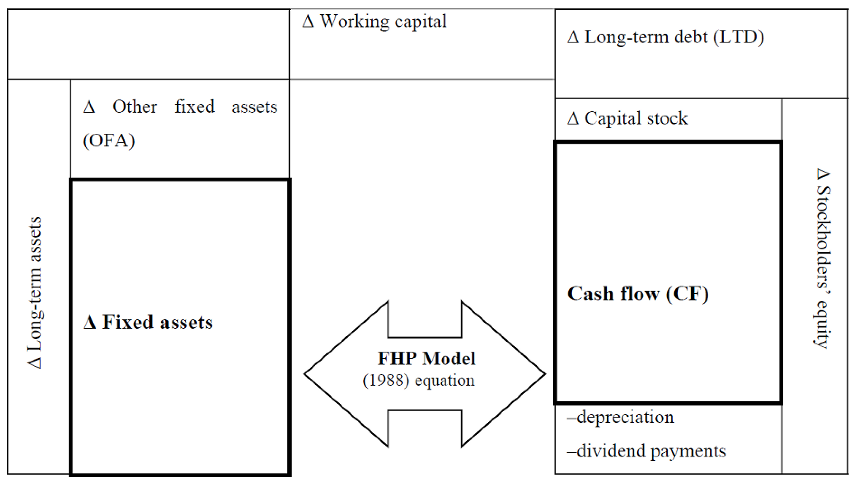
Figure 2.
Relation between the accounting identity and the ASI.

Table 1.
Regression of the complete accounting identity. The results of the OLS regression of Equation (2): for a set of 50,000 iterations of a Monte Carlo simulation of the randomly generated variables and .
Table 1.
Regression of the complete accounting identity. The results of the OLS regression of Equation (2): for a set of 50,000 iterations of a Monte Carlo simulation of the randomly generated variables and .
| Variable | Coef. | t |
|---|---|---|
| cash flow | 1.000 | ∞ *** |
| “rest” | 1.000 | ∞ *** |
| constant | 0.000 | ∞ *** |
| R2 | 1.000 |
*** denotes significance at the 1% level.
Table 2.
Descriptive statistics for the simulated variables.
| Cash Flows | Q | Investments | “Rest” | |
|---|---|---|---|---|
| Mean | 0.25 | 2.45 | 0.19 | −0.06 |
| Standard deviation | 0.10 | 0.20 | 0.11 | 0.12 |
Table 3.
Results of OLS estimation for for a set of 50,000 iterations of a Monte Carlo simulation of the randomly generated variables and .
Table 3.
Results of OLS estimation for for a set of 50,000 iterations of a Monte Carlo simulation of the randomly generated variables and .
| Whole Sample | Subsample Negative “Rest” | Subsample Positive “Rest” | Whole Sample | |||||
|---|---|---|---|---|---|---|---|---|
| Coef. | t | Coef. | t | Coef. | t | Coef. | t | |
| Cash flow | 0.452 *** (0.005) | 100.84 | 0.688 *** (0.004) | 161.85 | 0.824 *** (0.005) | 161.32 | 0.502 *** (0.003) | 150.41 |
| Dummy posit. “rest” × Cash flow | 0.666 *** (0.003) | 201.55 | ||||||
| Constant | 0.074 *** (0.001) | 61.14 | −0.033 *** (0.004) | −26.89 | 0.105 *** (0.001) | 96.08 | 0.024 *** (0.001) | 25.47 |
| R2 | 0.169 | 0.425 | 0.641 | 0.542 | ||||
| N | 50000 | 35484 | 14516 | 50000 | ||||
Robust standard errors are in parentheses. *** p < 0.01.
Table 4.
Results of the regression of Equation: . In column I, the estimation was run on a subsample where the amount of the “rest” or part missing from the complete accounting identity was restricted to approximately (±1%) 50% of the amount of cash flow. In column II, the ratio between “rest”/cash flows was allowed to vary between 0 and 1. Column III shows the result of the estimation for a subsample where the ratio “rest”/cash flows was allowed to vary between −5 and 5; Column IV is the estimation for the whole non-restricted sample, from a set of 50,000 iterations of a Monte Carlo simulation of the randomly generated variables.
| I | II | III | IV | |||||
|---|---|---|---|---|---|---|---|---|
| Variable | Coef. | t | Coef. | t | Coef. | t | Coef. | t |
| cash flow | 1.500 *** (0.0013) | 1115.05 | 1.003 *** (0.005) | 201.99 | 0.461 *** (0.005) | 101.23 | 0.452 *** (0.005) | 100.99 |
| Q | −0.000 (0.0004) | −0.70 | 0.007 *** (0.002) | 3.39 | 0.031 *** (0.002) | 14.02 | 0.031 *** (0.002) | 14.00 |
| constant | 0.000 (0.0011) | 0.64 | 0.039 *** (0.005) | 8.01 | −0.006 (0.006) | −0.99 | −0.003 (0.006) | −0.47 |
| N | 187 | 12,309 | 49,651 | 50,000 | ||||
| Adj-R2 | 0.999 | 0.769 | 0.174 | 0.172 | ||||
Robust standard errors in parentheses. *** denotes significance at 1% level.
Disclaimer/Publisher’s Note: The statements, opinions and data contained in all publications are solely those of the individual author(s) and contributor(s) and not of MDPI and/or the editor(s). MDPI and/or the editor(s) disclaim responsibility for any injury to people or property resulting from any ideas, methods, instructions or products referred to in the content. |
© 2023 by the author. Licensee MDPI, Basel, Switzerland. This article is an open access article distributed under the terms and conditions of the Creative Commons Attribution (CC BY) license (https://creativecommons.org/licenses/by/4.0/).
Share and Cite
MDPI and ACS Style
Sánchez-Vidal, F.J. A Cautionary Note on the Use of Accounting Semi-Identity-Based Models. J. Risk Financial Manag. 2023, 16, 389. https://doi.org/10.3390/jrfm16090389
AMA Style
Sánchez-Vidal FJ. A Cautionary Note on the Use of Accounting Semi-Identity-Based Models. Journal of Risk and Financial Management. 2023; 16(9):389. https://doi.org/10.3390/jrfm16090389
Chicago/Turabian StyleSánchez-Vidal, Francisco Javier. 2023. "A Cautionary Note on the Use of Accounting Semi-Identity-Based Models" Journal of Risk and Financial Management 16, no. 9: 389. https://doi.org/10.3390/jrfm16090389