
AIIB Investment and Economic Development of India: The Case of the Gujarat Road Project

1
Nanyang Centre for Public Administration, Nanyang Technological University, 50 Nanyang Avenue, Singapore 639798, Singapore
2
Department of Civil and Environmental Engineering, Imperial College London, London SW7 2AZ, UK
*
Author to whom correspondence should be addressed.
J. Risk Financial Manag. 2024, 17(2), 64; https://doi.org/10.3390/jrfm17020064
Submission received: 29 November 2023
/
Revised: 18 January 2024
/
Accepted: 30 January 2024
/
Published: 7 February 2024
(This article belongs to the Section Banking and Finance)
Abstract
:The purpose of this study is to verify whether the transportation infrastructure investment carried out by the Asian Infrastructure Investment Bank (AIIB) has promoted the economic development of its recipient countries. Since the establishment of the AIIB, its investments in infrastructure development, aimed at promoting economic growth in Asian developing countries, have garnered considerable attention. This study selects India, the largest recipient country of the AIIB, as the research object and chooses the Gujarat Road Project as the research case, since it is a completed infrastructure construction investment project in the transportation field. This paper provides an overview of the project’s operation and summarizes key factors in the project’s implementation. In the data analysis section, the per capita GDP is selected as the explained variable to measure economic development, and the LASSO regression method is used to select several variables that affect economic development. Moreover, the random forest model is used to obtain the causal relationship between road construction and the per capita GDP from 2001 to 2022. The results indicate that road construction in India has a significant positive effect on per capita GDP growth, the Gujarat Road Project supported by the AIIB also has a positive effect on per capita GDP growth, and this effect is stronger than that at the national level. The main contribution of this work is the validation of the investment strategy of the AIIB and the quantification of the economic contribution of AIIB investment projects to the local area.
1. Introduction
The Asian Infrastructure Investment Bank (AIIB) is a multilateral financial institution focusing on investing in the infrastructure construction sectors of developing countries. The AIIB states that its purpose is to promote the long-term sustainable development of developing countries and regions through investment in infrastructure construction (AIIB 2016). The AIIB has approved investments totaling USD 36.16 billion in 186 projects across 33 member countries. Energy (accounting for 19.27%), economic resilience (16.93%), and transportation (16.35%) are the top three investment sectors (AIIB 2023a). The above data are consistent with the AIIB’s aim of promoting the development of Asian developing countries through infrastructure investment.
It is noticeable that India is not only the member country with the second-largest voting power within the AIIB but also the largest recipient country of the AIIB. India expects to receive significant funding from the AIIB, and it is an ideal investment target for the AIIB too. India has received loans worth USD 8.65 billion from the Asian Infrastructure Investment Bank (AIIB), making it the largest recipient of AIIB loans (AIIB 2023b). Compared to other AIIB member countries, India has more loan plans for transportation infrastructure development, which is in line with India’s significant domestic economic disparities and vast territory. Clearly, one of India’s goals in joining the AIIB is to obtain a large amount of funding to build its transportation system and promote domestic economic development.
India has one of the largest road network systems in the world, and the AIIB’s investment in India’s transportation sector began in 2017. At that time, there was 5,897,671 km of road constructed in India and 289,194 km consisted of highways, occupying 4.91% (Ministry of Statistics and Program Implementation 2023). However, Unnikrishnan and Kattookaran (2020) stated that the infrastructure rating is only 3.0/10.0, which is highly unsatisfactory for the seventh-largest economy in the world (Unnikrishnan and Kattookaran 2020). To improve the transportation infrastructure, India invested USD 11.2 billion in infrastructure and increased the budget for road construction appropriation from USD 7.1 billion to USD 17.03 billion in 2017. In regard to the AIIB, its investment in transportation infrastructure has remained stable, from USD 664 million in 2017 to USD 946.5 million in 2022 (AIIB 2023c). The transportation projects approved by the AIIB mainly focus on rural and secondary roads, which is in line with the focus of India’s government-led road projects.
Although India has one of the largest transportation systems in the world, the level of infrastructure construction in India is not ideal, posing major challenges to India’s sustained high-speed economic growth. The existing literature also confirms the positive causal relationship between infrastructure construction and economic development. Therefore, the AIIB’s investment in road infrastructure construction is significant for India, and an analysis of the economic benefits of the road construction projects invested in by the AIIB can fill the gap in existing research about the AIIB. The choice of the Gujarat State Highway Project was based on it being the first investment project successfully completed by the AIIB in India. Additionally, there were government-led road construction projects in the region that served as a comparative reference.
The rest of this paper is organized as follows. Section 2 summarizes the existing literature on infrastructure investment, economic development and the role and operation of the AIIB. Section 3 presents the related data for India, the econometric methodologies used in the study and information about the Gujarat Road Project. Section 4 analyzes the empirical results. Finally, conclusions and predictions are presented in Section 5.
2. Literature Review
The existing literature mainly focuses on the causal relationship between foreign direct investment (FDI), infrastructure construction and economic development in theory. The literature on the AIIB mostly emphasizes the purpose of its establishment and its potential impact. However, there is limited research on the specific impact of the AIIB’s projects so far. Therefore, this study aims to address this research gap by reviewing the existing literature from three perspectives: the theoretical background of infrastructure investment and the AIIB, the current state of India’s infrastructure development, and the use of a random forest model and other regression methods.
2.1. Theoretical Background of Infrastructure Investment and the AIIB
The long-term causality between the total transportation infrastructure construction and economic development has been proven by a number of studies (Pradhan et al. 2013); (Maparu and Mazumder 2017); (Ghosh and Dinda 2022). Theoretically, infrastructure construction can promote economic development through three main mechanisms: enhancing factor productivity, attracting private investment, and improving regional connectivity. Firstly, the construction of transportation infrastructure can reduce transportation costs, increase the efficiency of other factors of production and intermediate goods, and invoke a multiplier effect. The study by Aschauer (1989) highlights that public expenditure on transportation infrastructure significantly enhances total factor productivity (Aschauer 1989). Leduc and Wilson (2013) found that government investments in highway projects can significantly boost the GDP in the medium term by enhancing productivity (Leduc and Wilson 2013). Additionally, the research by Chandra and Thompson (2000) suggests that road construction can elevate the economic development levels of regions that are directly affected (Chandra and Thompson 2000). Guild (2000) found that infrastructure investment drives economic development by promoting productive activities (Guild 2000).
Secondly, investors tend to prefer regions with better infrastructure as it leads to lower production costs, making local industries more competitive. Increased investments can scale up production, generate more employment opportunities and enhance market competitiveness. Through agglomeration effects, local industries’ factor productivity is strengthened, creating a positive cycle that drives economic development, as cited in the literature. Aiello et al. (2012) found that infrastructure construction will lower production costs for businesses, thereby promoting corporate investment (Aiello et al. 2012). Donaubauer et al. (2016) stated that only international aid focusing on infrastructure construction can increase foreign investment through this channel, while other types of aid cannot effectively improve infrastructure construction (Donaubauer et al. 2016). Khadaroo and Seetanah (2009) pointed out that sound transportation facilities are conducive to attracting foreign investment in developing countries, while infrastructure in other fields also has positive effects, but the degree is lower than for transportation facilities (Khadaroo and Seetanah 2009).
Finally, road infrastructure investment can improve regional connectivity, facilitating connections between regions and urban–rural areas. This not only aids in the circulation of goods and services but also promotes the mobility of talent and capital. Enhanced regional connectivity creates broader markets, making it easier for businesses to enter new markets and stimulating the development of local industries. This also contributes to regional integration into global and national economic systems, as evidenced by studies such as those by Suarez-Villa and Hasnath (1993), which found that infrastructure construction effectively promotes firms’ patent output and encourages industrial innovation (Suarez-Villa and Hasnath 1993). Sarania (2021) found that infrastructure construction can promote economic development by increasing the level of trade openness (Sarania 2021). Netirith and Ji (2022) pointed out that connectivity is important to link the community, regional integration, transportation and the direction of international trade import and export performance (Netirith and Ji 2022). Song (2021) found that railroads have a significant positive effect on the development of underdeveloped regions by connecting these regions with developed regions and bringing business opportunities (Song 2021). Aggarwal (2018) found that paving roads in India’s rural areas decreases the price of commodities and improves market integration (Aggarwal 2018).
In regard to the AIIB, there is a significant body of literature analyzing its role and operation. From the perspective of global order and governance, Gu (2017) and De Jonge (2017) stated that the AIIB complements the present international financing system (Gu 2017); (De Jonge 2017). Zhao (2016) stated that a notable contribution of the AIIB to global financial governance is its infusion of new funds, which can address the huge financing gap in underdeveloped regions in Asia, especially in the infrastructure sector (Zhao 2016). Meanwhile, China’s influence in the AIIB is a significant issue in the existing literature. Stephen and Skidmore (2019) find that the AIIB’s specific characteristics also reflect the increasing global influence of China’s political and economic order, and the AIIB’s focus on infrastructure-led development is itself an externalization of China’s domestic political and economic model (Stephen and Skidmore 2019). Regarding the future of the AIIB in South Asia, Kumar and Arora (2019) pointed out that this area faces the widest gaps in providing sustainable infrastructure and recommended that the AIIB should close these financing gaps (Kumar and Arora 2019).
The theoretical framework of this study is summarized in Figure 1. A number of studies have affirmed that infrastructure investment can drive economic development through multiple aspects; nevertheless, the specific economic effect of the AIIB’s transportation infrastructure investment in India warrants further scholarly investigation.
2.2. Current Infrastructure Construction in India
Regarding the current state of infrastructure construction in India, Saini and Giri (2022) found that the Indian government’s current budget for the infrastructure sector is Rs 100 trillion; it is committed to investing in infrastructure over the next 5 years, and over 6500 projects are expected to boost the country’s economy (Saini and Giri 2022). Unnikrishnan and Kattookaran (2020) state that the Indian government has made the FDI system in the infrastructure sector highly liberal. It allows 100% foreign direct investment into almost all infrastructure sectors, such as telecommunications and power generation, which can be handled through automatic routes (Unnikrishnan and Kattookaran 2020). However, Satyanand (2012) states that if the underlying operating environment is not politically and economically complete, a fully open FDI regime cannot be effective (Satyanand 2012). Hasnat (2021) points out that India’s commercial banks cannot be expected to invest in infrastructure construction due to the disproportionate amount of non-performing assets generated by overexposure to this sector (Hasnat 2021). Unnikrishnan and Kattookaran (2020) indicate that India’s infrastructure ranks only 66th out of 137 countries, with a score of 4.2 out of 7. For the world’s seventh-largest economy, these figures are disappointing. Moreover, due to the lack of infrastructure, India’s GDP experiences downward pressure of 1–2% per year (Unnikrishnan and Kattookaran 2020). Regarding the economic contribution of road construction, Aggarwal (2018) found that paving roads in India’s rural areas decreases the price of commodities and improves market integration (Aggarwal 2018).
2.3. Introduction to and Existing Literature on the Random Forest Model
The random forest model was first proposed by Ho (1995). The random forest method seeks to build multiple trees in randomly selected subspaces of the feature space, and the trees in different subspaces generalize their classification in a complementary manner (Ho 1995). Breiman (2001) introduced an important addition to random forest and pointed out that the generalization error of tree classifiers depends on the strength of the individual trees in the forest and the correlation between them. In addition, this study proposed that random forest can be used in regression to measure the importance of variables (Breiman 2001).
Regarding the basic idea of the random forest model, Stumpf and Kerle (2011) stated that the random forest model takes advantage of the high variance among individual trees, allows each tree to vote for class membership, and assigns the corresponding class based on the majority vote for the classification of unseen data (Stumpf and Kerle 2011). Levantesi and Piscopo (2020) pointed out that the random forest algorithm creates an ensemble of decision trees from any variant of the tree (Levantesi and Piscopo 2020). Once a specific learning set is defined, random forest applies random perturbations to the learning process and in this way produces variance between trees. Regarding the characteristics and advantages of random forest models, Levantesi and Piscopo (2020) stated random forest supports an understanding of the relationships between information variables and the target variable and highlights the importance of each factor (Levantesi and Piscopo 2020). Hong et al. (2016) stated that random forest, unlike other models, is able to provide several measures of feature importance, the most reliable of which is based on the magnitude of the drop in classification accuracy when the variable values are randomly permuted in the tree nodes (Hong et al. 2016). Stumpf and Kerle (2011) stated that random forest is based on ensembles of classification trees and exhibits many desirable properties, such as high accuracy, robustness against the overfitting of the training data, and integrated measures of variable importance. Such ensembles demonstrate robust performance and accuracy on complex datasets with little need for fine tuning (Stumpf and Kerle 2011).
In terms of the application of the random forest model in economic analysis, Tanaka et al. (2016) utilized this method to identify banks at risk of failing and to assess the vulnerability of industrial economic activities (Tanaka et al. 2016). Beutel et al. (2019) analyzed the use of the random forest method to predict banking crises and pointed out that random forest demonstrated the characteristic of strong in-sample fitting in practical applications, but it remains to be examined whether this is a sign of overfitting (Beutel et al. 2019).
In summary, the existing literature mainly focuses on the significance of the establishment of the AIIB and its impact on the international order, while less attention is paid to the development status and prospects of the AIIB in a specific region, such as South Asia. Before 2018, as the AIIB had only recently been established, the existing literature naturally focused on the analysis of its purpose and potential impact. However, while the AIIB has now been in operation for many years, there are still few studies on its current operating status, specific achievements and future development trends, and especially on the achievements of the AIIB in a member country. Moreover, it is necessary to verify the significance and possible results of the AIIB as proposed in the existing literature. Therefore, this study aims to analyze the current operating status and future prospects of the AIIB in India.
3. Data and Method
3.1. Data
The economic data for India are obtained from the database of Economists, and the data for Gujarat are derived from India’s Ministry of Statistics and Programme Implementation, the Directorate of Economy Statistics and the Government of Gujarat. These data are sourced and downloaded from the websites of the Statistics Times and the India Brand Equity Foundation (IBEF). This study utilizes the GDP per capita as an explanatory variable, and the personal consumption, unemployment rate, fixed investment, foreign direct investment (FDI), interest rate, and infrastructure rating as variables to measure the economic fundamentals of India. The reasons for choosing the per capita GDP as the explained variable are as follows. Firstly, the GDP is the indicator that most comprehensively reflects the level of the economy. Secondly, India is a populous country with a relatively high population growth rate; therefore, its total GDP will be significantly affected by population growth. Thus, this study uses the per capita GDP as a variable to measure the level of economic development. The purpose of selecting other economic variables is to construct the LASSO regression equation and random forest model together with the length of the roads, and to optimize the fitting effect of the model by adding these variables that may affect the GDP per capita. Regarding the control variables, the unemployment rate and FDI are chosen because road construction promotes economic development in these ways. The fixed investment and infrastructure rating are selected to control for other variables associated with infrastructure. Similarly, the interest rate and personal consumption are chosen to control for the factors that influence the per capita GDP. Due to the lack of data for Gujarat, this study uses only the GDP per capita, FDI and India’s national interest rate for the case analysis of the Gujarat Road Project.
The transportation infrastructure data of India are obtained from the official website of Pradhan Mantri Gram Sadak Yojana (PMGSY), which is a nationwide road construction plan for India, aimed at connecting numerous villages. This program began in 2001 and has constructed 703,352 km of road as of 2022. The government of India launched this program. Considering the continuity and reliability of the data, this study uses the length of road constructed by PMGSY to measure the transportation infrastructure of India. As a project invested in by the AIIB, the Gujarat Road Project is the first phase of Mukhya Mantri Gram Sadak Yojana (MMGSY), which is a road construction program implemented in 2016 by the North States Government to connect rural villages. For the road data before 2016–2017, this study selects the PMGSY road mileage at the Gujarat state level for filling. Therefore, the sum of the road length of the Gujarat Road Project, PMGSY and MMGSY is used to measure the transportation infrastructure of Gujarat.
As indicated in Figure 2, India’s GDP per capita grew steadily from 2001 to 2022, with the exception of 2020, due to the COVID-19 pandemic. However, the private consumption per capita increased more slowly than the GDP per capita. Regarding the unemployment rate, it dropped from 2001 to 2015 and experienced a brief fluctuation in 2016–2017; it then grew until 2020. In recent years, unemployment has fallen rapidly to a historically low level.
In regard to investment, Figure 3 shows that the level of fixed investment increased steadily in this period, with the exception of 2020. The growth rate of fixed investment reached a trough in 2008 and 2013 and then rebounded and peaked in 2011 and 2018. Although there was a recession in 2020, it quickly rebounded to the peak of this period. In contrast, inward direct investment, or FDI, is much more volatile. In general, the change trend of FDI is consistent with that of fixed investment, but serious deviations occurred in 2008, 2017 and 2020. This may have been due to the hedging behavior of global capital during the economic crisis. Regarding the interest rate, it maintained a downward trend, except in the subprime crisis. Finally, the infrastructure rating rose from 2001 to 2007 and remained stable until 2014. After a fluctuation, it began increasing again after 2017.
For Gujarat, this study only selects the GDP per capita and its growth rate and FDI as economic data variables due to the lack of reliable data. As Figure 4 shows, the GDP per capita of Gujarat continued to increase and only slowed in 2020 and 2021. Moreover, it indicates that Gujarat experienced a great deal of FDI inflowing in 2011, 2020 and 2021. Compared with the overall situation of India, the FDI inflow in Gujarat was roughly consistent with the FDI at the country level, and only in 2020–2021 was there a lag in FDI transmission as Figure 5 indicates. The total road length in Gujarat, on the other hand, began to grow rapidly in 2016. Before 2016, the construction of PMGSY gradually leveled off, so there was no noticeable change in the total length of road. After the implementation of MMGSY and the Gujarat Road Project, the total length of road started to increase significantly.
Presenting detailed data on the road length, Figure 6 indicates the length of road completed by PMGSY from 2001 to 2022, which has grown steadily. For Gujarat, Figure 7 provides detailed road length data. As the figure shows, the road constructed by the MMGSY project accounts for most of the road length in Gujarat, and the proportion represented by the AIIB-funded road construction project is also significant. In regard to the different length components, the construction of PMGSY stagnated from 2016 to 2022, while the roads built by MMGSY gradually increased during this time period. The Gujarat Road Project, invested in by the AIIB, started in 2017 and was completed in 2019.
3.2. Methodology
This study aims to analyze the above data at the national and regional levels using a random forest model. Firstly, based on the economic data and PMGSY road data at the national level for India, a regression model of the influence of the road length on the GDP per capita is established, and the impact of the increase in road length on the GDP per capita is predicted according to this model. Secondly, via the causal relationship and regression equation obtained at the national level, the data of Gujarat are analyzed to solve the problems of missing data and the small data size. Through the analysis at the local level of Gujarat, the impact of the Asian Infrastructure Investment Bank (AIIB)’s investment on the local GDP per capita is obtained, thus quantifying the contribution of the AIIB to local economic development.
3.2.1. LASSO Method
This study also employs stepwise analysis and the LASSO (Least Absolute Shrinkage and Selection Operator) model to screen the listed economic variables in India, aiming to improve the effectiveness of the regional-level analysis. Stepwise regression is a procedure that sequentially selects or removes features based on their statistical significance and contribution to the model’s predictive power. The method aims to strike a balance between model accuracy and simplicity by iteratively adding or removing features until the optimal subset is achieved. In this study, stepwise regression is used to select variables at the national level with the Akaike information criterion (AIC) (Liu et al. 2021). LASSO is a regularization technique that adds a penalty term to the ordinary least squares regression objective equation, which forces the coefficients of some features to be reduced towards zero, effectively performing feature selection (Tibshirani 1996). The details are as follows:
In this function, is the adjusted coefficient of the explanatory variable; λ represents the strength of the model’s penalty for overfitting and is selected by k-1 fold cross-validation. The core of LASSO is to reduce the number of selected variables and the complexity of the model on the basis of minimizing the residual sum of squares, so as to avoid the problem of overfitting. Considering that the LASSO method is more suitable for a small number of highly correlated variables than stepwise regression, LASSO is used directly in the analysis of the regional data, and the selection is made according to the effect of LASSO and stepwise regression at the national level.
3.2.2. Random Forest Model
Random forest is an ensemble learning method that constructs a large number of decision trees based on randomly sampled subsets of the training data and features. Tin Kam Ho (1995) was the first to propose the random forest model and stated that multiple classifiers can be used to deal with a single classifier’s bias (Ho 1995). The random forest model aggregates the predictions of individual trees and forms a combination of random decision trees to make the final prediction.
The random forest model generates decision trees according to the following methods:
- Using the bootstrap sample method, for the training set of size N, N training samples are randomly selected from the training set as the training set of each tree.
- If there are M features, M feature dimensions (m << M) are randomly selected from M when each node is split, and the best features (maximizing information gain) among these m feature dimensions are used to segment the nodes. During the growth of the forest, the value of m remains constant (Breiman 1996).
The fitting effect of the random forest model depends on the correlation and classification ability of the classification trees. The weaker the correlation between classification trees, the stronger the classification of each tree and the better the fitting effect of the model. The strength of correlation and classification is determined by the number of feature dimensions m. Therefore, the construction of the model requires the identification of the appropriate feature dimensions (Breiman 2001).
Since randomly different bootstrap samples are used to construct each classification tree, approximately 1/3 of the training instances are not involved in the generation of k trees, which are called out-of-bag (OOB) samples of k trees. OOB samples are cross-verified to calculate the OOB error rate of the random forest model, and m is screened based on this standard. One of the advantages of the random forest model is that it is not necessary to set up additional test groups. For regression, random forest takes the average of the predicted values of each tree as the result of the prediction. Another advantage of the random forest model is that it can determine the importance of the selected variables. The partial importance score for one variable is obtained by removing this variable and then subtracting the percentage of votes for the correct class in the OOB data and removing the variable from the percentage of votes for the correct class in the unchanged OOB data (Breiman 2001).
The random forest model deals with the regression relationship between variables using an ensemble decision tree, which effectively reduces the impact of noise and overfitting, and it does not need to eliminate variables in advance. In addition, random forest models can maintain accuracy in the absence of data (Ho 1995). Therefore, this study chooses to use a random forest model to analyze the economic and infrastructure development data in India, in order to determine whether road infrastructure construction has a positive impact on the important economic indicator of the per capita GDP and to quantify the contribution of the road length to per capita GDP growth. Based on this, we assess whether the Gujarat highway project has driven local per capita GDP growth by increasing the road length, and we quantify its contribution, thereby analyzing the economic impact of investment by the Asian Infrastructure Investment Bank (AIIB) on the local economy. In summary, this study puts forward two hypotheses. At the national level, we posit the following hypothesis.
H1:
An increase in road length will lead to a significant increase in per capita GDP at the national level.
For the investment of the Asian Infrastructure Investment Bank (AIIB) in Gujarat, the following hypothesis is proposed.
H2:
An increase in road length due to the construction of the Gujarat Road Project will lead to a significant increase in per capita GDP in Gujarat.
4. Results Analysis
In this study, the GDP per capita is selected as the explained variable to represent the economic level, and other variables, including the variable of time, are set as alternative explanatory variables. The reason for choosing the GDP per capita is that the GDP is a variable that comprehensively reflects the economic level of a country. However, India is a populous country with a rapidly growing population, which greatly influences its GDP. Therefore, this study selects the per capita GDP as the dependent variable to measure the economic development level of the country.
4.1. Analysis at the National Level
Firstly, the data at the national level of India were processed. Below, we show the correlation of variables calculated.
As Figure 8 indicates, the GDP per capita, time, fixed investment, private consumption per capita and road length are strongly correlated, and the interest rate is negatively correlated with the above variables. The infrastructure rating, FDI and unemployment rate are less correlated with other variables, and the total factor productivity growth is weakly correlated.
This study uses stepwise regression and the LASSO method to select the best combination of the above variables, so as to build a model to identify which variables contribute to the improvement of India and Gujarat’s economics. Firstly, the AIC is used here to filter out the best regression equation and avoid overfitting in stepwise regression. After regression and optimization, backward regression is selected, and the optimal regression equation is as follows:
As Table 1 indicates, the infrastructure rating, inward direct investment, total factor productivity growth, lending interest rate, gross fixed investment and PMGSY road length of India are selected as explanatory variables, while the year, private consumption per capita and unemployment rate are excluded to avoid overfitting.
Compared with stepwise regression, the use of LASSO regression resulted in different outcomes. Under the optimal regularization parameter value, a lambda of 27.8255, the regression equation is given as follows:
Using this equation, this study generates the predicted value of the explained variable, y_hat_cv, and the result is listed below. Moreover, the coefficient of determination is 0.9944468, which is very close to 1, so it can be determined that the regression equation obtained by the LASSO model has achieved a very good fitting effect. Moreover, stepwise regression is more suitable for situations with a large sample size and low intercorrelation among independent variables. It can explain the relationships between the independent variables and the dependent variable well. LASSO regression, on the other hand, is more appropriate for situations where the independent variables are strongly correlated with each other. Considering that most variables of this study are strongly correlated and the number of variables is small, this study selects Equation (2) as the regression equation at the national level of India.
Next, this study performs the regression of variables using the random forest model. Using this model, we can determine which variables contribute more to the growth of the GDP per capita. Figure 9 presents the result.
As the figure indicates, the PMGSY road length and fixed investment are the variables that contribute to the growth of the GDP per capita, with contributions of 13.37% and 12.15%. The variables of time and consumption follow closely behind, contributing 12.00% and 11.15%, respectively. Other eliminated variables contribute less than 10%, which confirms the reliability of the previous LASSO regression.
To further verify the reliability of the model, this study employs a random forest model to make predictions based on the existing data, and we then compare the predicted values with the actual data to obtain the distribution data of residuals. Let ResidualAsPrctOfYhat be the ratio of residuals to predicted values; taking a confidence level of 0.05, the results are calculated and shown in Figure 10.
It is found that most of the residuals are distributed in the confidence interval (−0.05, 0.05), and the overall distribution pattern conforms to a normal distribution. Hence, it is reasonable to confirm that this random forest model is reliable.
Next, this study generates the partial dependence of the main explanatory variable, the PMGSY road length. According to Figure 11, the positive impact of the road mileage on the per capita GDP is most prominent in the range of 270 to 550 thousand kilometers, and it is relatively flat outside this range. When the length of constructed roads is less than 270,000 km, each additional 1000 km of road length leads to a per capita GDP increase of USD 0.74. For road lengths between 270,000 and 550,000 km, each additional 1000 km of road length results in a per capita GDP increase of USD 2.60. However, for road lengths exceeding 550,000 km, the impact of the road length on the GDP is not significant. Notably, India entered this stage after 2018. Therefore, we can conclude that, at the national level in India, an increase in road mileage has a positive effect on the per capita GDP that exhibits a pattern of first increasing marginal returns followed by decreasing marginal returns. When the road length is less than 550 thousand kilometers, the characteristics of an economy of scale and scope of infrastructure construction play a major role, while, beyond this threshold, the law of diminishing marginal returns dominates.
Building on the previous analysis, the variable of fixed investment, with the second-highest contribution, was added, and the results are presented in Figure 12. In the figure, the lighter colors correspond to higher values of per capita GDP, and the denser gradients represent faster per capita GDP growth. It can be seen that the per capita GDP growth is supported by the growth of both the road length and fixed investment, and the GDP growth mainly occurs in the range of road length of 270,000 to 550,000 km and fixed investment from 2.8 to 4 trillion LCU. This confirms the existence of the marginal effect of increasing returns followed by diminishing returns in infrastructure investment and construction, which reflects the significant economies of scale in the early development stage of this field and the tendency towards overcapacity and reduced investment efficiency due to diminishing marginal returns in the later stage.
Adding the variable of the interest rate, Figure 13 shows the growth of the GDP per capita as affected by the road length and interest rate. It is indicated that a decrease in the interest rate will result in the growth of the GDP per capita, and this effect only occurs when the interest rate is smaller than approximately 10.6%. When the interest rate is higher than this threshold, the increase in the GDP per capita caused by the road length is slow and cannot exceed USD 5200. Therefore, the positive impact of road construction on GDP per capita growth can only be fully achieved within a sufficiently low interest rate range.
Although the variable of FDI does not have a significant effect on GDP per capita growth, it is still included here for comparison with the region of Gujarat. As Figure 14 shows, both FDI and road construction contribute to the growth of the GDP per capita, but the effect of FDI is less significant. Similarly to the effect of the interest rate, an increase in FDI has no effect when it is more than USD 50 billion. Overall, it is clear that a variable without a significant contribution, as Figure 9 indicates, can only affect the growth of the GDP per capita within a certain range.
In general, the road infrastructure has a significant positive effect on the growth of the GDP per capita, which proves H1. Moreover, this positive effect is supported by the effect of fixed investment. The economic contribution of road construction shows the characteristics of an economy of scale when the length is small and diminishing marginal utility when the length is large. Hence, it is reasonable to state that transportation infrastructure construction promotes economic development in India.
4.2. Analysis of Gujarat
In this section, the same method is used to analyze the data of Gujarat State. Firstly, the correlation of different variables is calculated as below.
As Figure 15 shows, the GDP per capita is correlated with time, the MMGSY and AIIB’s road length and the total road length. The road length variables of different projects are correlated with each other. Due to the small number of variables and strong correlation, we choose the LASSO method to generate the regression equation.
Here, the variables of PMGSY and MMGSY denote the road length of the PMGSY and MMGSY program in Gujarat during 2016–2022, and the variable of AIIB denotes the length of road constructed in the Gujarat Road Project invested in by the AIIB. The regression equation generated by the LASSO method is as follows:
The lambda for this equation is 3.5938, and the coefficient of determination is 0.9946663, which is a very satisfactory result. It is worth noting that the regression equation obtained by the LASSO regression method only retains the variable corresponding to the construction of roads for the AIIB investment project, focusing on the road variables that are strongly correlated with each other, which is the focus of this study.
By building the random forest model, the contributions of the variables can be revealed. As Figure 16 indicates, the variable of MMGSY contributed the most, amounting to 4.69%. The contribution of the variable of AIIB, denoting the length of road constructed by the Gujarat Road Project, was the second largest at 4.46%. Therefore, it can be considered that every kilometer of AIIB-funded road built in Gujarat contributes 4.46% per unit of GDP per capita growth.
However, due to the insufficient data sample, the residual distribution of the model is not ideal. Although most of the results are within the confidence interval of (−0.05, 0.05), the distribution does not show normality as Figure 17 indicates. In regard to the partial dependence, on the whole, it is reasonable to suggest that the road construction project invested in by the AIIB has a positive effect on Gujarat’s economic growth. As Figure 18 shows, when the constructed road length is less than approximately 4200 km, it has no effect on the growth of the GDP per capita. Moreover, if the road length is over 4200 km, an increase of one thousand kilometers in road length will result in a per capita GDP increase of approximately USD 14.29, which is higher than the effect of the constructed road length at a national level. Therefore, it is reasonable to conclude that Hypothesis 2 is confirmed and the economic effect of the AIIB’s road investment is greater than the effect of the previous road investment of PMGSY. This means that the AIIB’s investment in transportation infrastructure has a stronger economic effect than the investment of India’s government.
Next, other variables are added and the economic effect on the GDP per capita of both the road length of the Gujarat Road Project and other variables is considered. Figure 19 measures the contribution to the GDP per capita of the AIIB’s project and the MMGSY program’s road length. As the figure shows, the AIIB and MMGSY variables each require one another to be sufficiently large in order to function optimally. When the road length of the AIIB project is lower than approximately 6000 km, it has no effect with the variable MMGSY on the GDP per capita, and the effect of the MMGSY variable will also be reduced. For MMGSY, when its road length is lower than 10,000 km, the situation is the same. The upper right corner of Figure 19 shows that the increase in the AIIB and MMGSY road length has a very significant positive effect on per capita GDP growth, where the variable of AIIB exceeds 10,000 km and MMGSY exceeds 30,000 km. Overall, it is obvious that horizontal complementarity and the economies of scale characteristic exist between the road construction projects, which is likely due to the extreme underinvestment in transportation infrastructure construction in the state of Gujarat.
However, the economic effect is not significant when the variable of FDI is added, as Figure 20shows. The positive effect on the GDP per capita of FDI mainly emerges when it is lower than USD 10 billion; when the road length of the AIIB’s project is over approximately 11,000 km, the positive effect of the FDI’s increase on the GDP growth per capita is more obvious.
To summarize, although the statistical significance of the results is affected due to the limited data, it can still be concluded that the AIIB’s investment in Gujarat has achieved positive economic effects, and the effect is greater than that of the Indian government’s previous investment. In addition, the Gujarat Road Project and the MMGSY program in the same period show complementarity with the characteristics of economies of scale. As the length of the roads constructed by these two projects increases, the positive effects of the two on the economy are also strengthened.
According to the above results, we can draw the following preliminary conclusions. Firstly, in the field of road infrastructure investment in India, we observe the characteristics of economies of scale at low levels, while, at high levels, we see diminishing marginal utility. At present, road construction in India is in the latter stage; therefore, large-scale road construction at the national level needs to be carefully considered. Secondly, investment in roads in Gujarat is insufficient. The investment of the AIIB has a positive economic effect that is greater than that at the national average level after reaching a certain scale, and it is complementary to the MMGSY program carried out by the government of Gujarat. This result shows that there is no conflict between the investment of the AIIB and that of the local government in Gujarat, and they can even promote each other so as to generate better economic utility.
4.3. Analysis of Other Economic Variables
In addition to the per capita GDP, this study examines the impact of road construction on other economic variables. Firstly, based on the theoretical background, we posit that road construction projects may stimulate economic development from three aspects: consumption, employment, and attracting foreign investment. Utilizing national-level data from India, the study finds that road construction projects have a positive influence on consumption, while not exhibiting a significant impact on employment and attracting foreign investment. For the correlation between road construction and per capita consumption, the regression equation obtained through the stepwise regression method demonstrates a better fit compared to the equation derived from the LASSO method, with a higher coefficient of determination (0.9925554 > 0.1247556). The equation derived from stepwise regression is as follows:
The random forest model illustrates the contributions of individual variables to the variations in per capita consumption. As depicted in Figure 21, the most influential variable is fixed capital investment, accounting for 12.27% of the contribution, while the road projects of the PMGSY contribute 11.81%. It can be inferred that the construction of each kilometer of road in India can stimulate an 11.81% increase in per capita consumption. Furthermore, as shown in Figure 22, the residual distribution of the model is ideal, with the majority falling within the confidence interval of (−0.05, 0.05), aligning well with a normal distribution.
Regarding the partial dependence, a clear positive correlation is observed between road construction and per capita consumption, as shown in Figure 23. When the road mileage is less than 500,000 km, the promotional effect of road construction on consumption is highly pronounced. However, as the road mileage exceeds 500,000 km, this promotional effect begins to diminish.
Building upon the preceding analysis, the incorporation of the highest-contributing fixed investment variable yields the outcomes presented in Figure 24. In the figure, lighter hues correspond to elevated per capita consumption, while denser gradients signify swifter growth. It is discernible that both road construction and fixed capital investment distinctly increase per capita consumption, manifesting economies of scale in the initial phases of development and experiencing diminishing marginal benefits in subsequent stages.
Following the introduction of the interest rate variable to the analysis, Figure 25 delineates the impact of the road length and interest rates on per capita GDP growth. The findings indicate that a decline in interest rates precipitates an upswing in per capita consumption, with this effect occurring solely when interest rates hover around 10.6% or lower. Analogous to its influence on GDP, the positive impact of road construction on per capita consumption growth can be fully realized only within a sufficiently low interest rate range.
Upon the inclusion of the foreign investment variable, as depicted in Figure 26, both road construction and foreign investment make conspicuous contributions to the increase in per capita consumption. However, foreign investment contributes minimally to consumption growth when it is below USD 15 billion and surpasses USD 40 billion. This suggests that, for consumption growth, foreign investment also adheres to a pattern of escalating marginal benefits succeeded by diminishing returns.
Regarding the AIIB’s investments in the state of Gujarat, an analysis cannot be carried out here due to the lack of data on unemployment rates and per capita consumption. Similar to the national level, foreign investment does not show a significant impact of road construction. In conclusion, road construction notably stimulates consumption, while it does not show significant effects on employment and foreign investment. Further in-depth research is warranted in this regard.
4.4. Analysis Based on the Time Series Forecasting Model
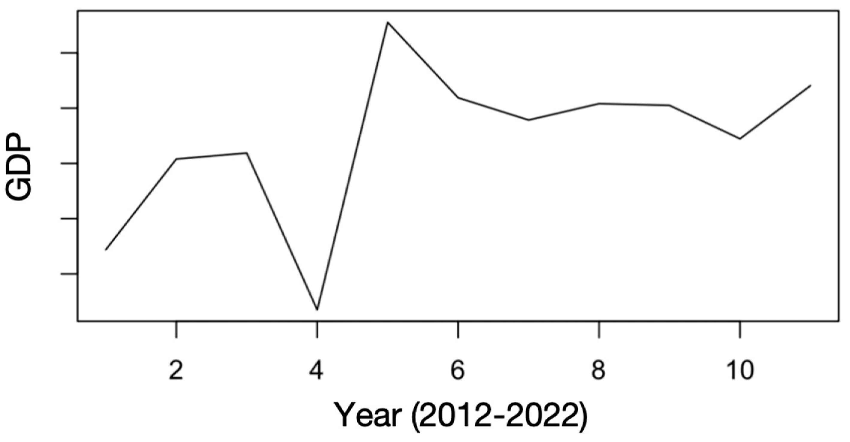
The autoregressive integrated moving average (ARIMA) method is used to build a time series forecasting model to investigate temporal patterns, trends, and delayed effects of infrastructure investments on economic growth. The ARIMA (2,0,1) model fits the series best due to having the lowest AIC and BIC. It shows that 2 AR terms and 1 MA term are considered. AR term means it is regressed on its own lagged values, and MA term means it is modeled via its own imperfectly predicted values of current and previous times. In general, it means the effect of infrastructure investment on GDP development will appear within a two year period and is influenced by imperfection (errors) in the last year.
The time series fitting plot also shows that there is an upward trend in the future which is reflected by the consecutive investment of AIIB on infrastructure in the past years (Figure 27).
5. Discussion and Conclusions
This study analyzes India’s transportation infrastructure construction data and related economic data using the methods of stepwise regression, LASSO and random forest. The two hypotheses proposed in this study, H1 and H2, are verified. Firstly, road construction in India has a significant positive impact on the per capita GDP and can promote per capita GDP growth. Secondly, the investment of the AIIB in Gujarat State has achieved positive economic effects, and the specific quantitative results are higher than those at the national level.
The main contribution of this study is the demonstration, through the collection and organization of relevant data, that road infrastructure construction has a positive effect on economic growth in India, and to quantify the investment results of the AIIB in Gujarat, which offers a useful supplement to existing research on the AIIB. Regarding the implementation of the Gujarat Road Project, the overall completion rate of this project is high, and it has saved a significant amount of funds for the local government. Moreover, the communication mechanism developed by the AIIB, aimed at effectively engaging local grassroots political organizations and the public, deserves to be promoted. However, the specific environmental protection standards in the implementation of the project rely on the legal system of the recipient country and it has not adopted uniform and up-to-date standards, which may present a challenge in the implementation framework of the project.
Regarding the economic effect of transportation infrastructure investment in India, firstly, this study proves that road construction by the government of India has a significant positive effect on the GDP per capita, while, in recent years, this effect has been weakened due to the improvements in infrastructure investment. Concerning the Gujarat Road Project, the road construction funding by the AIIB achieved a greater economic effect than that at the national level, and each one thousand kilometers of road length will result in a per capita GDP increase of approximately USD 14.29. Moreover, unlike at the national level in India, road construction in Gujarat has not yet reached the stage of diminishing marginal utility, and there is a certain degree of complementarity between infrastructure investments by the AIIB and local programs. This result indicates that although road construction at the national level is relatively sufficient, there are still significant economic benefits to investing in road infrastructure in states such as Gujarat, especially in its rural areas. Finally, regarding other economic indicators, this study finds that road infrastructure construction has a stimulating effect on consumption but does not exhibit a significant impact on employment and attracting foreign investment. This suggests that further discussions are needed to delve into the mechanisms through which road infrastructure investments contribute to economic development. This study suggests that future infrastructure investments by the AIIB in India should focus on regions with good government efficiency and some public investment projects, but still lacking in infrastructure development.
The application of the random forest model in this study achieved the expected results. Firstly, the random forest model solved the endogeneity problem and directly calculated the contribution of the road mileage to per capita GDP growth. Moreover, with the use of the random forest model, we were able to obtain the economic effect of the road project in Gujarat invested in by the AIIB, despite insufficient data. There are still many shortcomings in this study that need to be addressed. Firstly, due to the insufficient sample size of the data, we were unable to construct a consistent analysis model of road construction and economic development that is applicable to both the national and local levels, as envisioned in theory. The models generated from the data at the national level and from the data of Gujarat differ and have not been unified. Secondly, due to the lack of data, the analysis results regarding the investment effects of the AIIB still have limitations in terms of model reliability and predictive ability. The variables used in the model are correlated and the effect of the LASSO regression method is to be determined. The random forest model also has room for further improvement. Finally, both LASSO and the random forest model lack an analysis of the economic impact caused by time factors. In subsequent studies, a deep learning time series model will be considered for prediction, so as to build a comprehensive prediction analysis model. We hope that future research can obtain better results on the basis of supplementing local-level data, thereby providing recommendations for the future development of the AIIB.
Author Contributions
Conceptualization, J.C.; methodology, J.C. and B.C.; software, J.C. and B.C.; validation, B.C.; formal analysis, J.C. and B.C.; investigation, J.C. and B.C.; resources, J.C. and B.C.; data curation, J.C. and B.C.; writing—original draft preparation, J.C. and B.C.; writing—review and editing, J.C. and B.C.; visualization, J.C.; supervision, B.C.; project administration, B.C.; funding acquisition, B.C. All authors have read and agreed to the published version of the manuscript.
Funding
This research received no external funding.
Data Availability Statement
Due to confidentiality, data is not available to public.
Conflicts of Interest
Authors do not have conflicts of interest on this study.
References
- Aggarwal, Shilpa. 2018. Do Rural Roads Create Pathways out of Poverty? Evidence from India. Journal of Development Economics 133: 375–95. [Google Scholar] [CrossRef]
- Aiello, Francesco, Alfonsina Iona, and Leone Leonida. 2012. Regional Infrastructure and Firm Investment: Theory and Empirical Evidence for Italy. Empirical Economics 42: 835–62. [Google Scholar] [CrossRef]
- AIIB. 2016. Asian Infrastructure Investment Bank. Articles of Agreement. Beijing: AIIB. [Google Scholar]
- AIIB. 2023a. Our Projects. Available online: https://www.aiib.org/en/projects/list/index.html (accessed on 14 April 2023).
- AIIB. 2023b. Our Projects. Available online: https://www.aiib.org/en/projects/list/year/All/member/India/sector/All/financing_type/All/status/Approved (accessed on 14 April 2023).
- AIIB. 2023c. Our Projects. Available online: https://www.aiib.org/en/projects/list/year/All/member/All/sector/Transport/financing_type/All/status/Approved (accessed on 14 April 2023).
- Aschauer, David Alan. 1989. Is Public Expenditure Productive? Journal of Monetary Economics 23: 177–200. [Google Scholar] [CrossRef]
- Beutel, Johannes, Sophia List, and Gregor von Schweinitz. 2019. Does Machine Learning Help Us Predict Banking Crises? Journal of Financial Stability 45: 100693. [Google Scholar] [CrossRef]
- Breiman, Leo. 1996. Bagging predictors. Machine Learning 24: 123–40. [Google Scholar] [CrossRef]
- Breiman, Leo. 2001. Random Forests. Machine Learning 45: 5–32. [Google Scholar] [CrossRef]
- Chandra, Amitabh, and Eric Thompson. 2000. Does Public Infrastructure Affect Economic Activity? Evidence from the Rural Interstate Highway System. Regional Science and Urban Economics 30: 457–90. [Google Scholar] [CrossRef]
- De Jonge, Alice. 2017. Perspectives on the Emerging Role of the Asian Infrastructure Investment Bank. International Affairs 93: 1061–84. [Google Scholar] [CrossRef]
- Donaubauer, Julian, Birgit Meyer, and Peter Nunnenkamp. 2016. Aid, Infrastructure, and FDI: Assessing the Transmission Channel with a New Index of Infrastructure. IDEAS Working Paper Series from RePEc; Vienna: Research Centre International Economics. [Google Scholar]
- Ghosh, Prabir Kumar, and Soumyananda Dinda. 2022. Revisited the Relationship Between Economic Growth and Transport Infrastructure in India: An Empirical Study. Indian Economic Journal 70: 34–52. [Google Scholar] [CrossRef]
- Gu, Bin. 2017. Chinese Multilateralism in the AIIB. Journal of International Economic Law 20: 137–58. [Google Scholar] [CrossRef]
- Guild, Robert L. 2000. Infrastructure Investment and Interregional Development: Theory, Evidence, and Implications for Planning. Public Works Management & Policy 4: 274–85. [Google Scholar]
- Hasnat, Tanzeem. 2021. Infrastructure Investment in India: Squaring Theory, Data and Common Sense. Indian Economic Journal 69: 174–78. [Google Scholar] [CrossRef]
- Ho, Tin Kam. 1995. Random Decision Forests. Paper presented at 3rd International Conference on Document Analysis and Recognition, Montreal, QC, Canada, August 14–16; vol. 1, pp. 278–82. [Google Scholar]
- Hong, Haoyuan, Hamid Reza Pourghasemi, and Zohre Sadat Pourtaghi. 2016. Landslide Susceptibility Assessment in Lianhua County (China): A Comparison between a Random Forest Data Mining Technique and Bivariate and Multivariate Statistical Models. Geomorphology 259: 105–18. [Google Scholar] [CrossRef]
- Khadaroo, Jameel, and Boopen Seetanah. 2009. The Role of Transport Infrastructure in FDI: Evidence from Africa Using GMM Estimates. Journal of Transport Economics and Policy 43: 365–84. [Google Scholar]
- Kumar, Nagesh, and Ojasvee Arora. 2019. Financing Sustainable Infrastructure Development in South Asia: The Case of AIIB. Global Policy 10: 619–24. [Google Scholar] [CrossRef]
- Leduc, Sylvain, and Daniel Wilson. 2013. Roads to Prosperity or Bridges to Nowhere? Theory and Evidence on the Impact of Public Infrastructure Investment. NBER Macroeconomics Annual 27: 89–142. [Google Scholar] [CrossRef]
- Levantesi, Susanna, and Gabriella Piscopo. 2020. The Importance of Economic Variables on London Real Estate Market: A Random Forest Approach. Risks 8: 112. [Google Scholar] [CrossRef]
- Liu, Yingxia, Gerard B. M. Heuvelink, Zhanguo Bai, Ping He, Xinpeng Xu, Wencheng Ding, and Shaohui Huang. 2021. Analysis of Spatio-Temporal Variation of Crop Yield in China Using Stepwise Multiple Linear Regression. Field Crops Research 264: 108098. [Google Scholar] [CrossRef]
- Maparu, Tuhin Subhra, and Tarak Nath Mazumder. 2017. Transport Infrastructure, Economic Development and Urbanization in India (1990–2011): Is There Any Causal Relationship? Transportation Research. Part A, Policy and Practice 100: 319–36. [Google Scholar] [CrossRef]
- Ministry of Statistics and Program Implementation. 2023. Basic Road Statistics of India; Public Document. Available online: https://www.mospi.gov.in (accessed on 14 April 2023).
- Netirith, Narthsirinth, and Mingjun Ji. 2022. Analysis of the Efficiency of Transport Infrastructure Connectivity and Trade. Sustainability 14: 9613. [Google Scholar] [CrossRef]
- Pradhan, Rudra P., Neville R. Norman, Yuosre Badir, and Bele Samadhan. 2013. Transport Infrastructure, Foreign Direct Investment and Economic Growth Interactions in India: The ARDL Bounds Testing Approach. Procedia, Social and Behavioral Sciences 104: 914–21. [Google Scholar] [CrossRef]
- Saini, Shalu, and Jagat Narayan Giri. 2022. Infrastructure Development in India: The Way Ahead. Journal of Infrastructure Development 14: 37–44. [Google Scholar] [CrossRef]
- Sarania, Rahul. 2021. Interactions among Infrastructure, Trade Openness, Foreign Direct Investments and Economic Growth in India. Journal of Infrastructure Development 13: 21–43. [Google Scholar] [CrossRef]
- Satyanand, Premila Nazareth. 2012. India, FDI and Infrastructure: Some Observations on the Past Twenty Years. Review of Market Integration 4: 239–82. [Google Scholar] [CrossRef]
- Song, Ge. 2021. Road versus Rail: Assessing the Implications of Transport Infrastructure for Spatial Growth Pattern in China’s Megaregions. Journal of Urban Planning and Development 147: 04020050. [Google Scholar] [CrossRef]
- Stephen, Matthew D., and David Skidmore. 2019. The AIIB in the Liberal International Order. The Chinese Journal of International Politics 12: 61–91. [Google Scholar] [CrossRef]
- Stumpf, André, and Norman Kerle. 2011. Object-Oriented Mapping of Landslides Using Random Forests. Remote Sensing of Environment 115: 2564–77. [Google Scholar] [CrossRef]
- Suarez-Villa, Luis, and Syed A. Hasnath. 1993. The Effect of Infrastructure on Invention: Innovative Capacity and the Dynamics of Public Construction Investment. Technological Forecasting & Social Change 44: 333–58. [Google Scholar]
- Tanaka, Katsuyuki, Takuji Kinkyo, and Shigeyuki Hamori. 2016. Random Forests-Based Early Warning System for Bank Failures. Economics Letters 148: 118–21. [Google Scholar] [CrossRef]
- Tibshirani, Robert. 1996. Regression Shrinkage and Selection via the Lasso. Journal of the Royal Statistical Society. Series B, Methodological 58: 267–88. [Google Scholar] [CrossRef]
- Unnikrishnan, Nishija, and Thomas Paul Kattookaran. 2020. Impact of Public and Private Infrastructure Investment on Economic Growth: Evidence from India. Journal of Infrastructure Development 12: 119–38. [Google Scholar] [CrossRef]
- Zhao, Hong. 2016. AIIB Portents Significant Impact on Global Financial Governance. ISEAS Perspective 41: 11. [Google Scholar]
Figure 1.
The theoretical framework of economic effect of infrastructure investment.
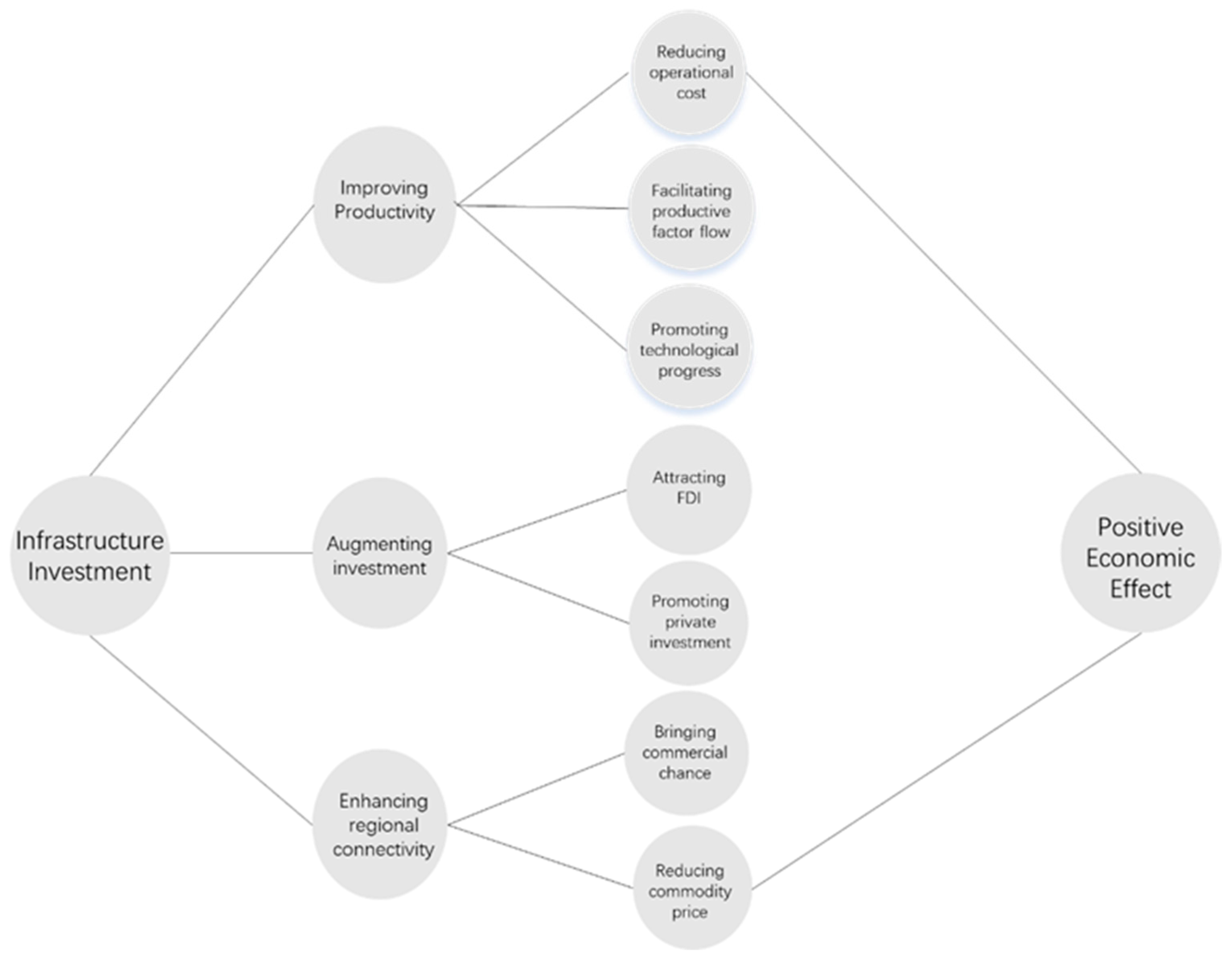
Figure 2.
Livelihood of India in 2001–2022. Data: Economist Intelligence Unit.
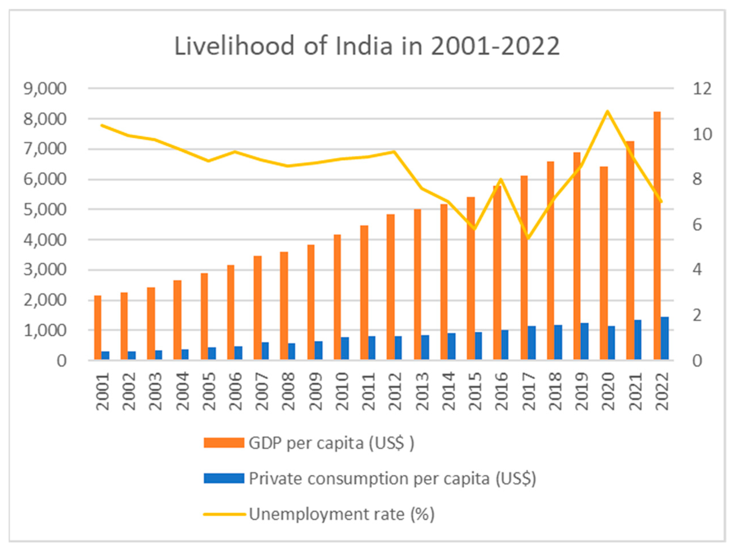
Figure 3.
Investment of India in 2001–2022. Data: Economist Intelligence Unit.
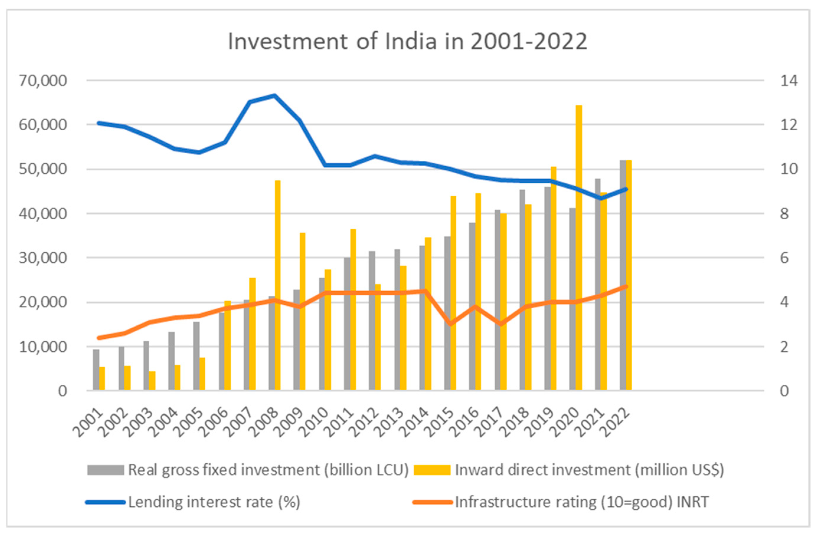
Figure 4.
GDP per capita and GDP growth of Gujarat.

Figure 5.
FDI inflow and total project road length of Gujarat. Data: Statistics Times, IBEF http://omms.nic.in/ (accessed on 23 April 2023); https://rwdbihar.gov.in/SchemeMMGSY.aspx (accessed on 23 April 2023); https://www.aiib.org/en/projects/details/2017/approved/_download/India/AIIB-IND-L00025A-Gujarat-MMGSY-PCN-November-12-2020.pdf (accessed on 23 April 2023).

Figure 6.
PMGSY road length in India.
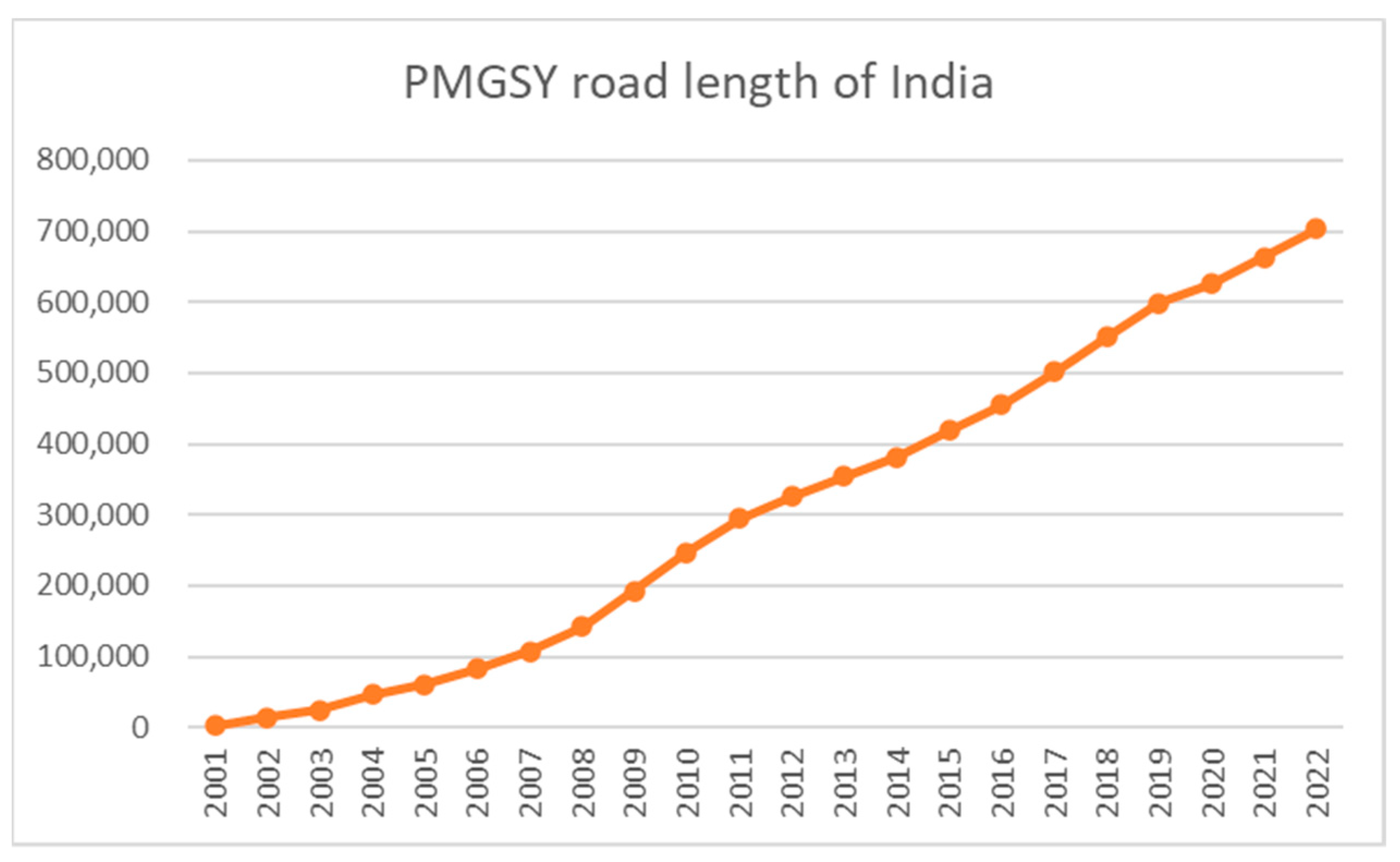
Figure 7.
Length of PMGSY, MMGSY and Gujarat Road Project completed road in Gujarat. Data: http://omms.nic.in/ (accessed on 23 April 2023); https://rwdbihar.gov.in/SchemeMMGSY.aspx (accessed on 23 April 2023); https://www.aiib.org/en/projects/details/2017/approved/_download/India/AIIB-IND-L00025A-Gujarat-MMGSY-PCN-November-12-2020.pdf (accessed on 23 April 2023).

Figure 8.
Correlation of variables at national level.
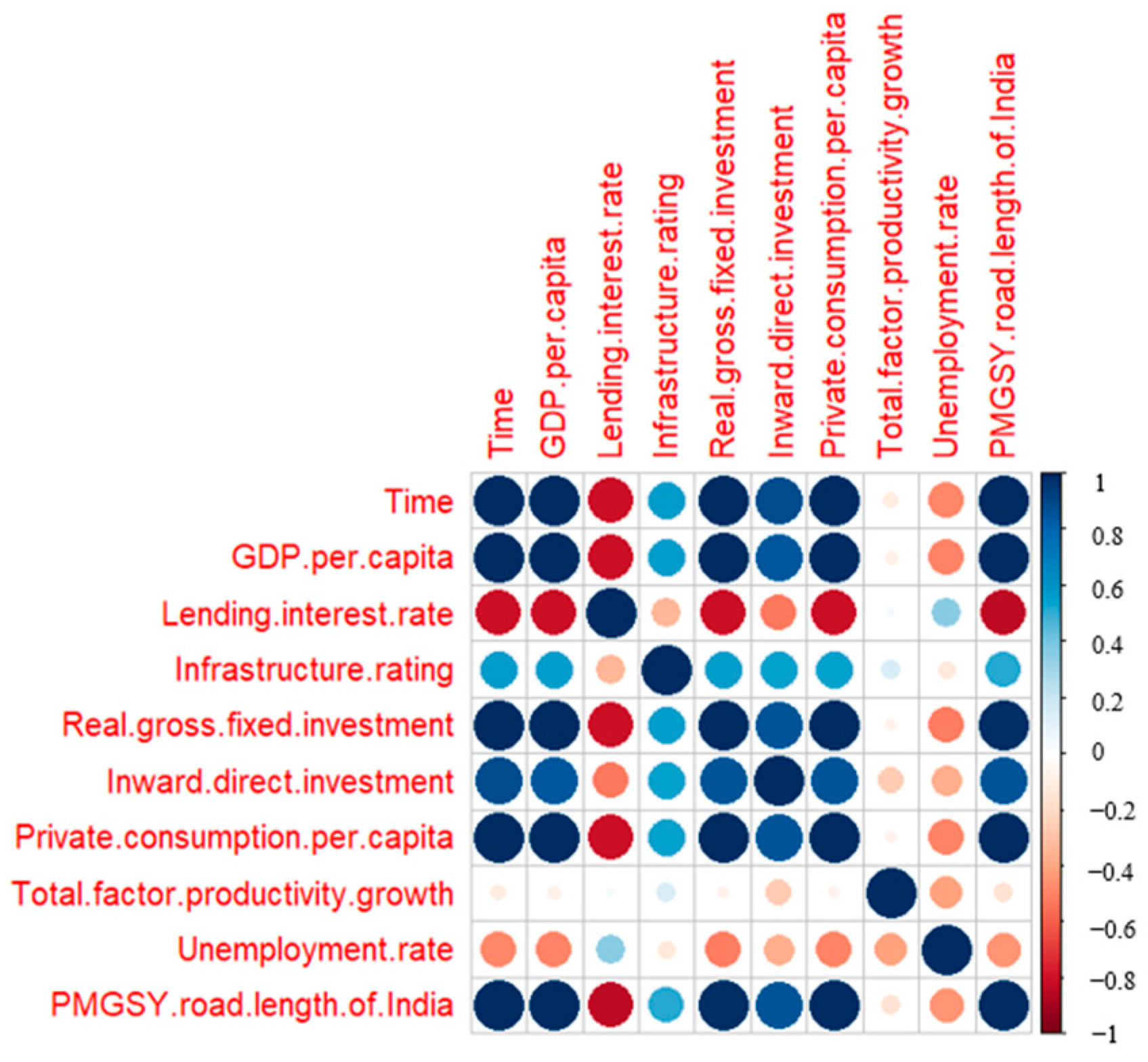
Figure 9.
Contribution of variables to GDP per capita.
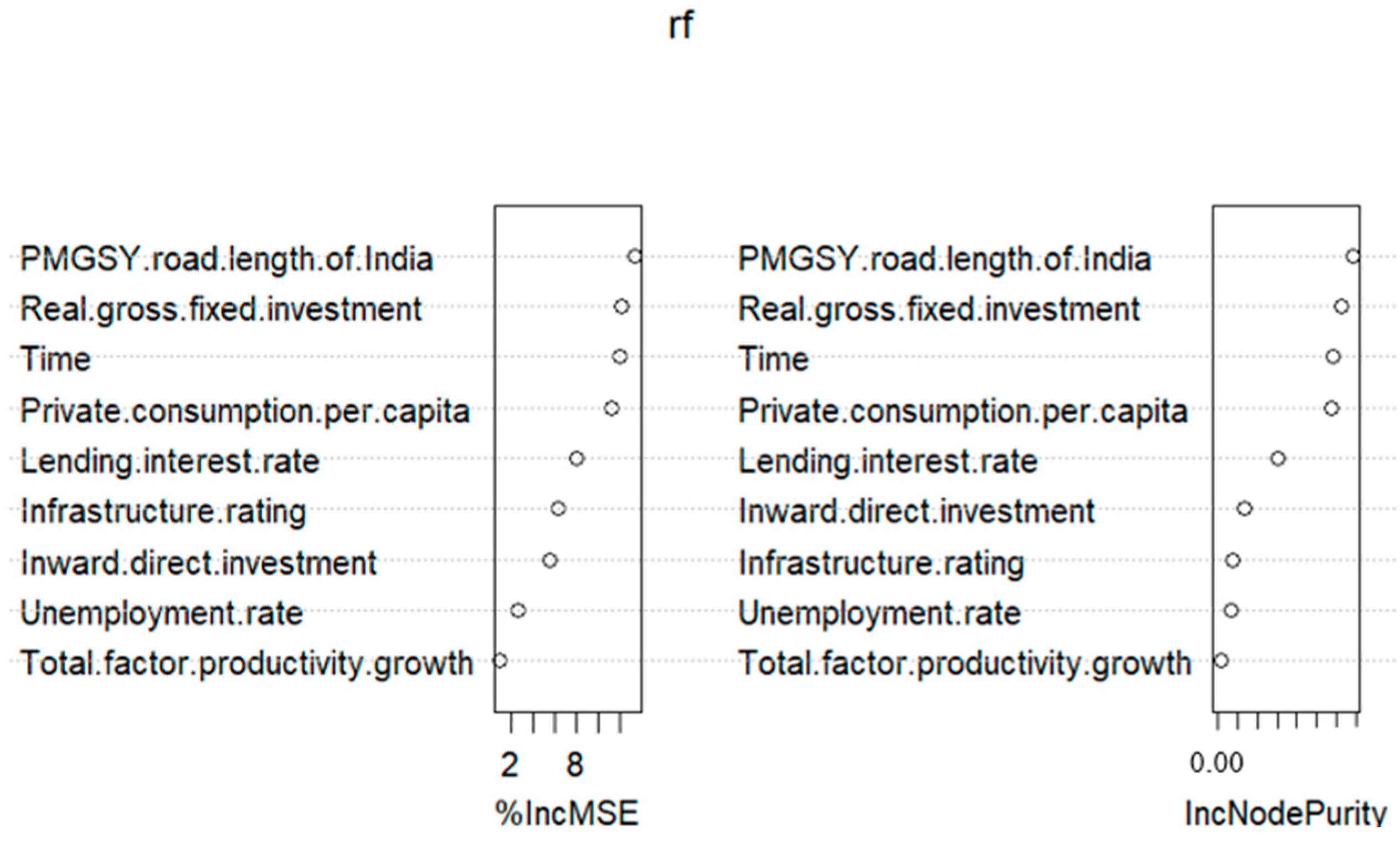
Figure 10.
Histogram of ResidualAsPrctOfYhat.

Figure 11.
Partial dependence on PMGSY road length of India. 0.74 GDP/1000 km road; 2.6 GDP/1000 km road.
Figure 11.
Partial dependence on PMGSY road length of India. 0.74 GDP/1000 km road; 2.6 GDP/1000 km road.
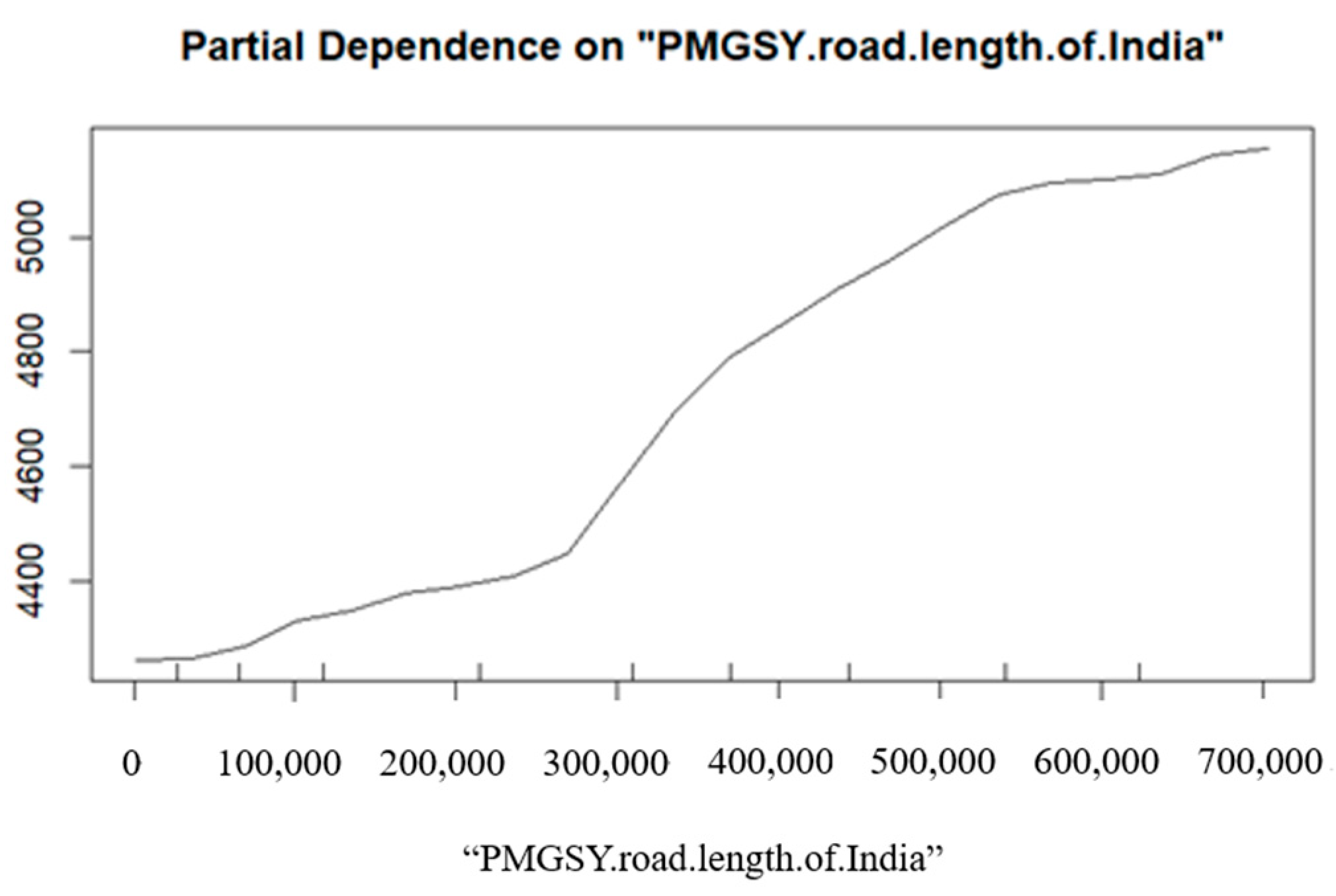
Figure 12.
Partial plot of PMGSY road length and fixed investment. Unit: kilometer; million USD.
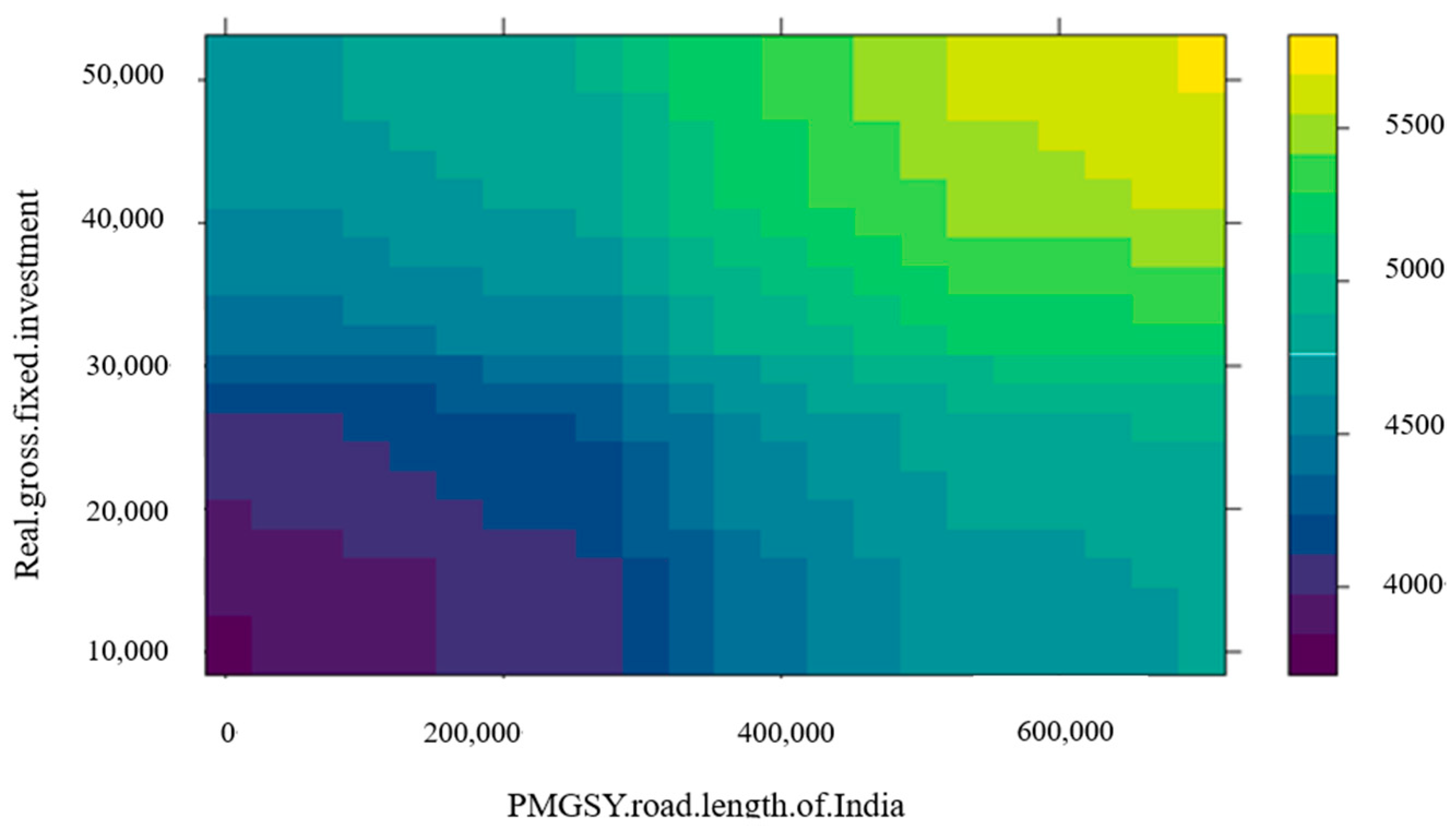
Figure 13.
Partial plot of PMGSY road length and interest rate. Unit: kilometer; percent.

Figure 14.
Partial plot of PMGSY road length and inward direct investment. Unit: kilometer; million USD.
Figure 14.
Partial plot of PMGSY road length and inward direct investment. Unit: kilometer; million USD.
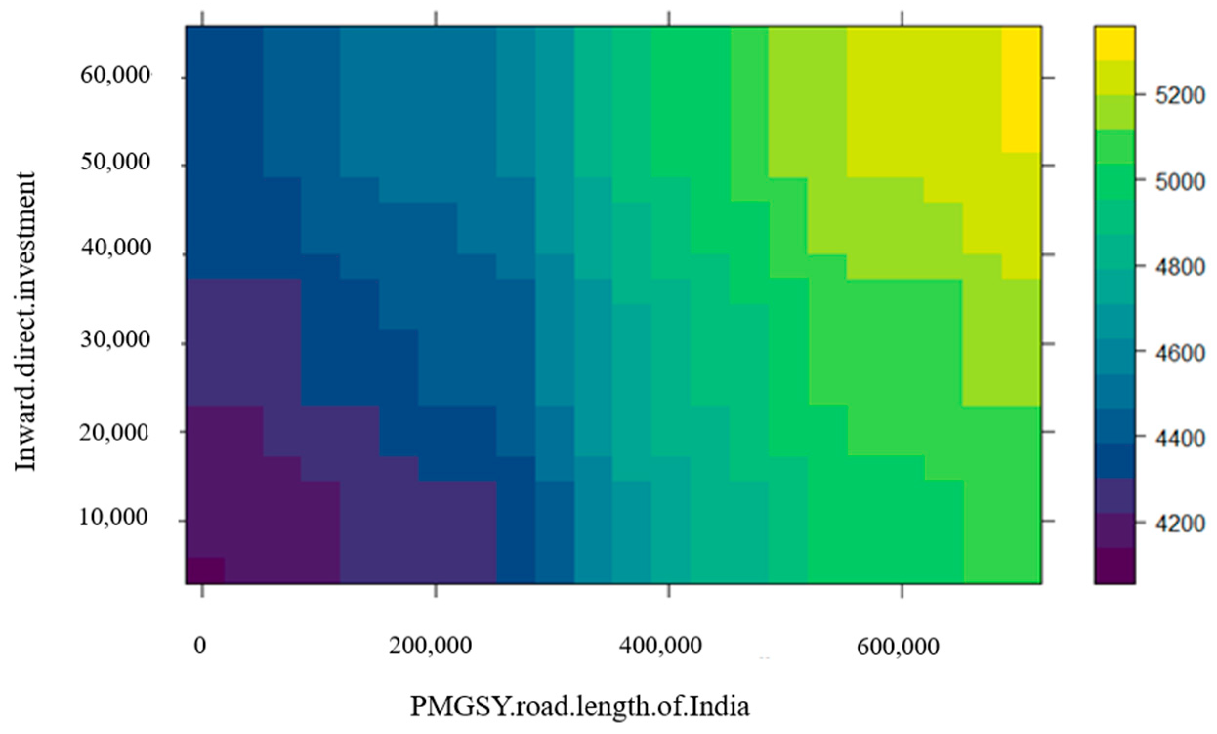
Figure 15.
Correlation of variables for Gujarat.

Figure 16.
Contribution of variables to GDP per capita in Gujarat.
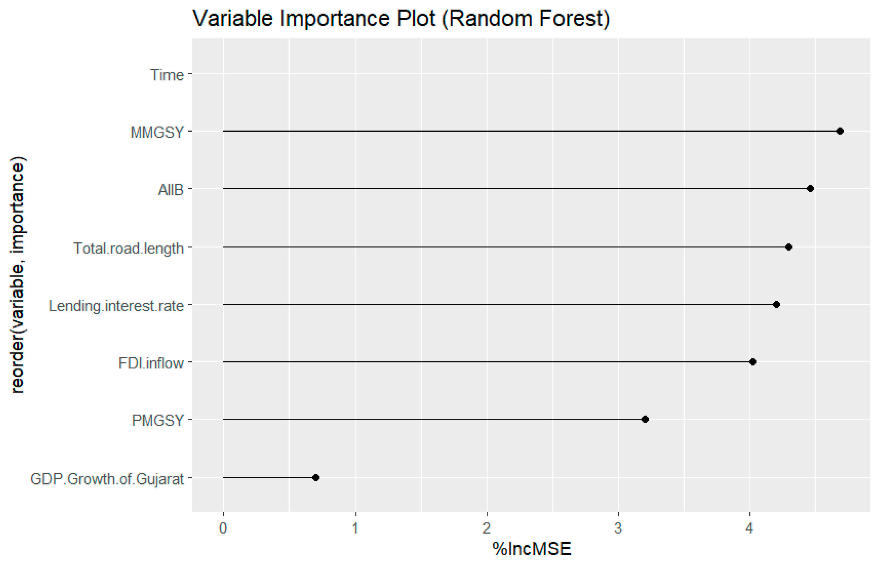
Figure 17.
Histogram of ResidualAsPrctOfYhat.
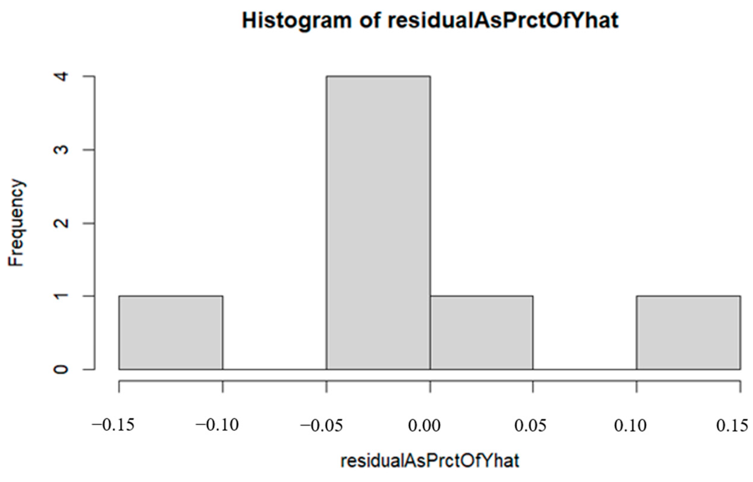
Figure 18.
Partial dependence on PMGSY road length in India.
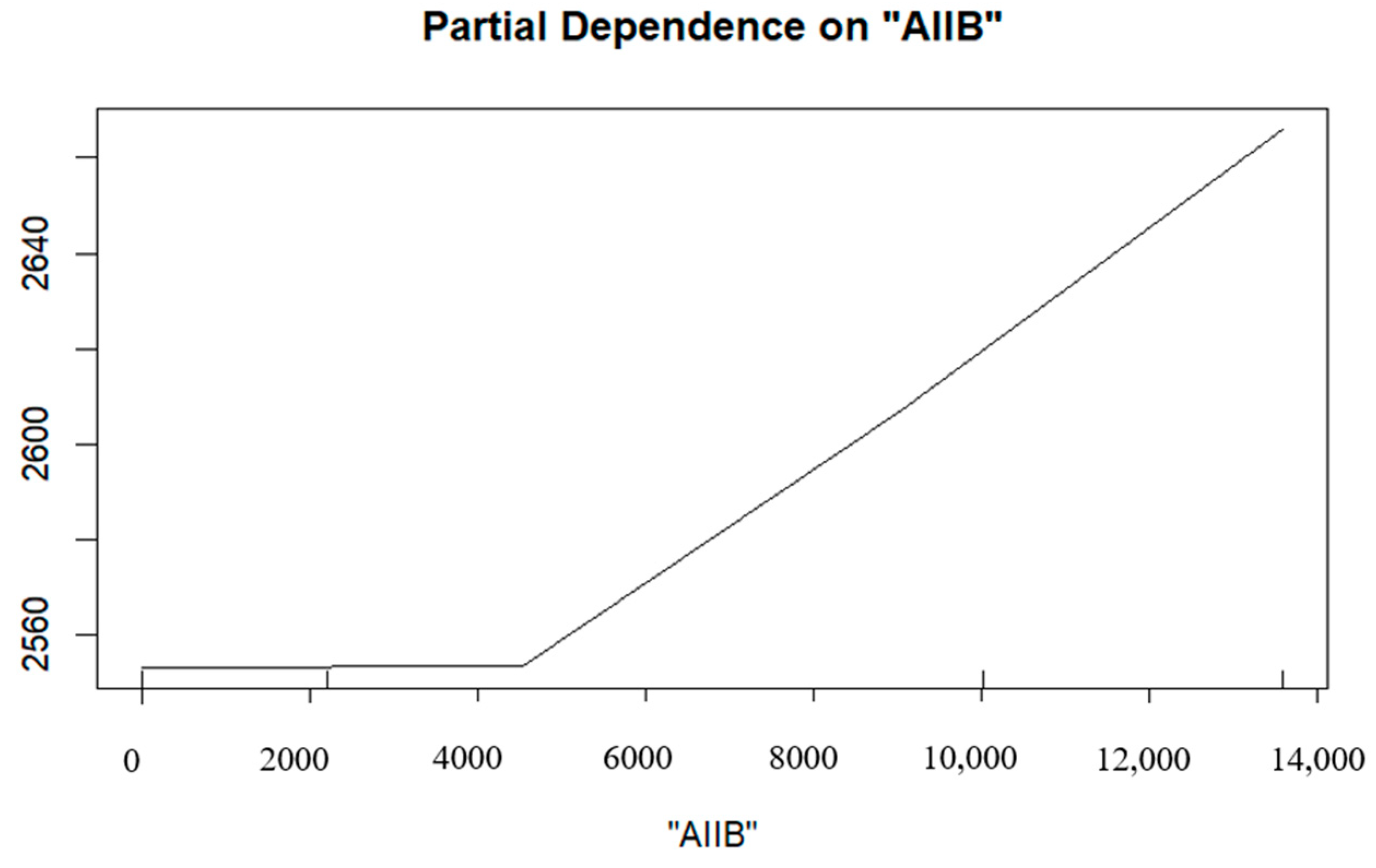
Figure 19.
Partial plot of AIIB and MMGSY road length. Unit: kilometer.
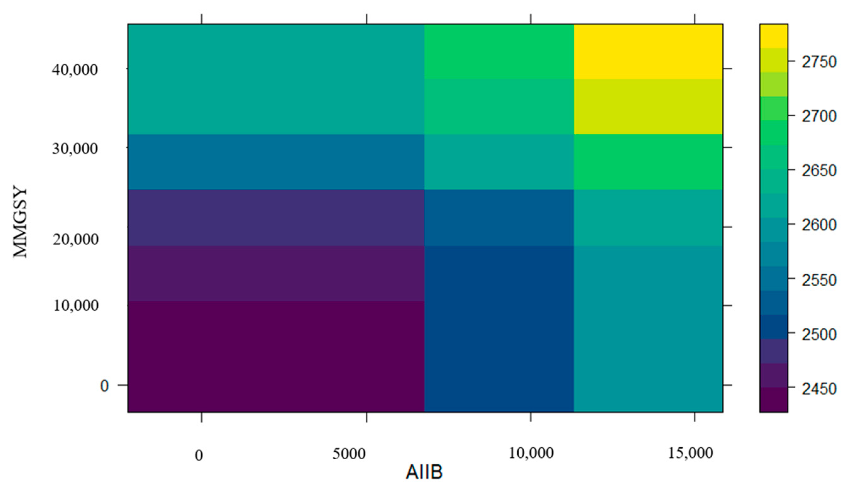
Figure 20.
Partial plot of AIIB and MMGSY road length. Unit: kilometer; billion USD.
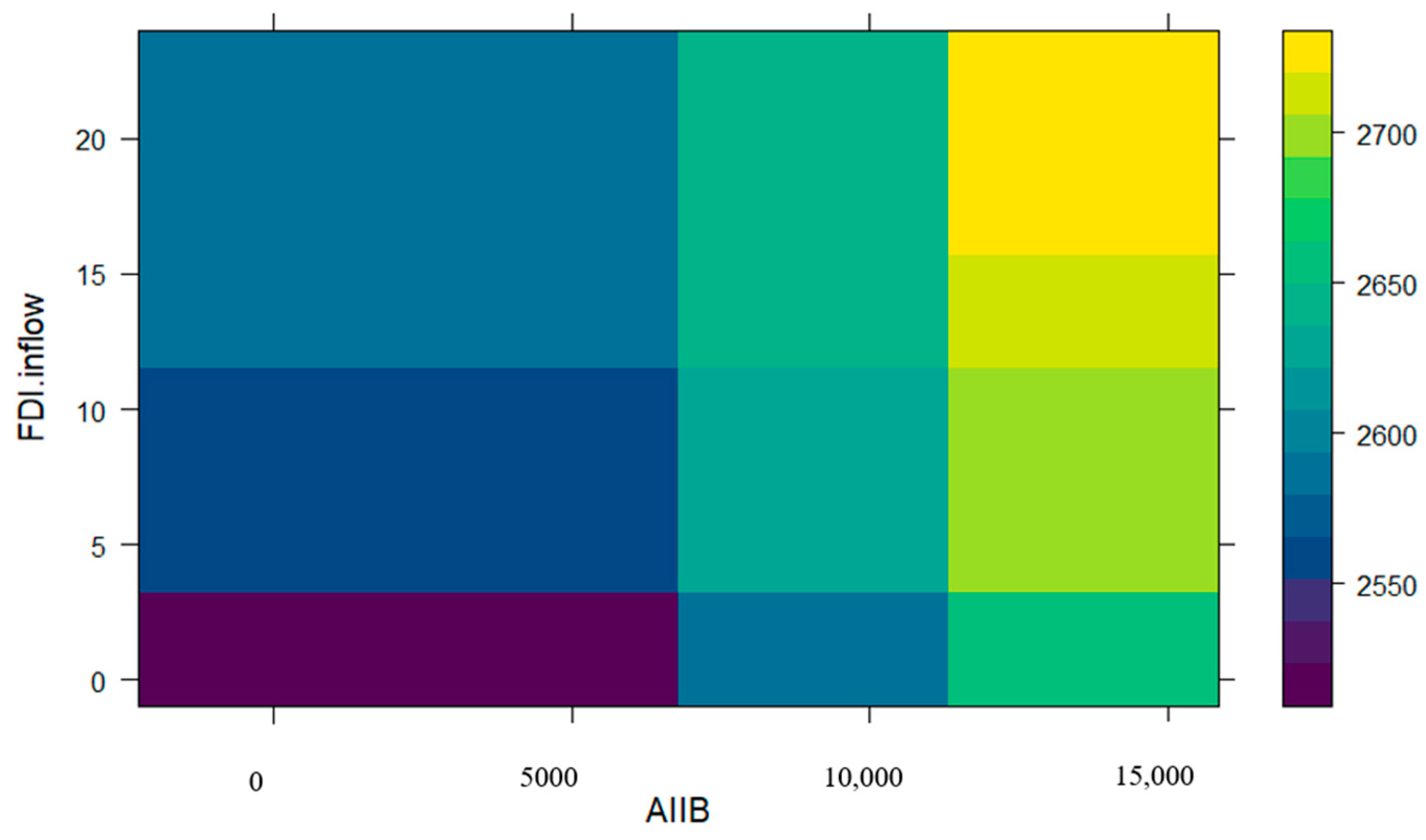
Figure 21.
Contribution of variables to personal consumption per capita.

Figure 22.
Histogram of ResidualAsPrctOfYhat.
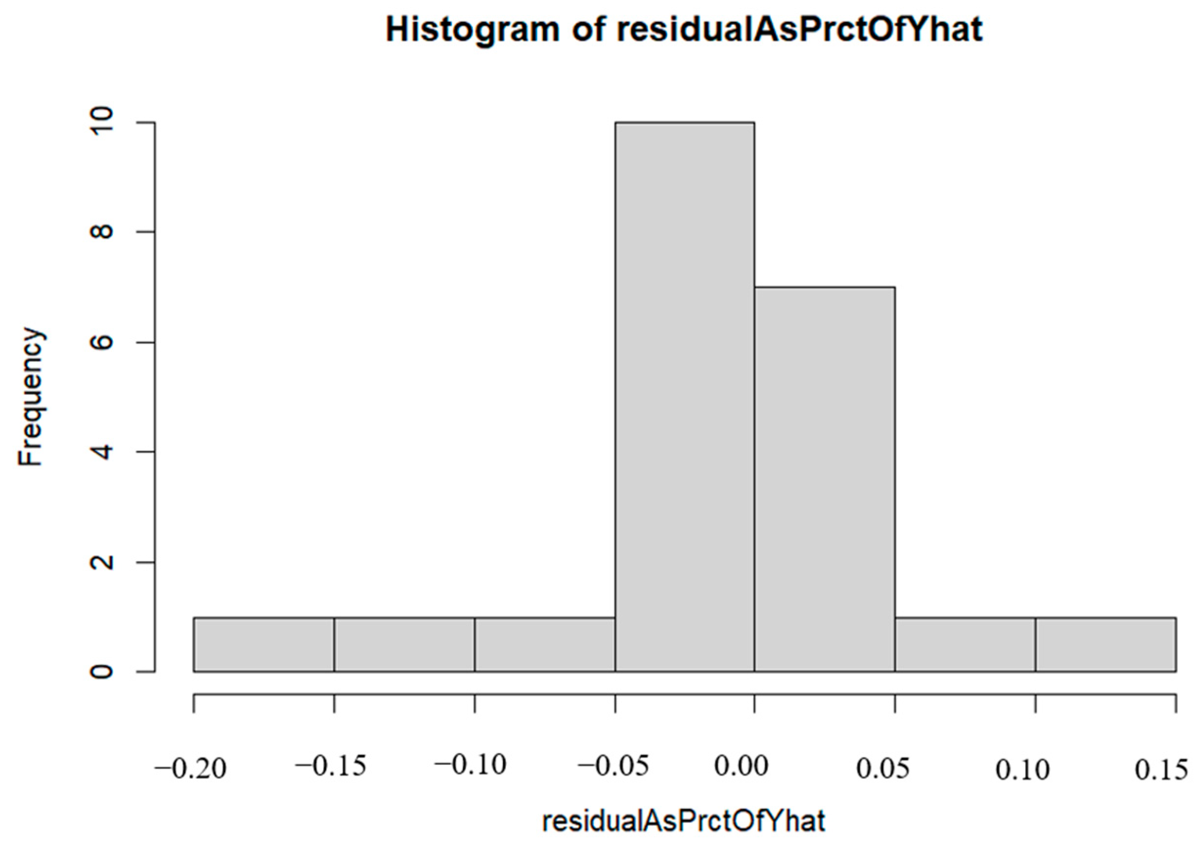
Figure 23.
Partial dependence on PMGSY road length in India.
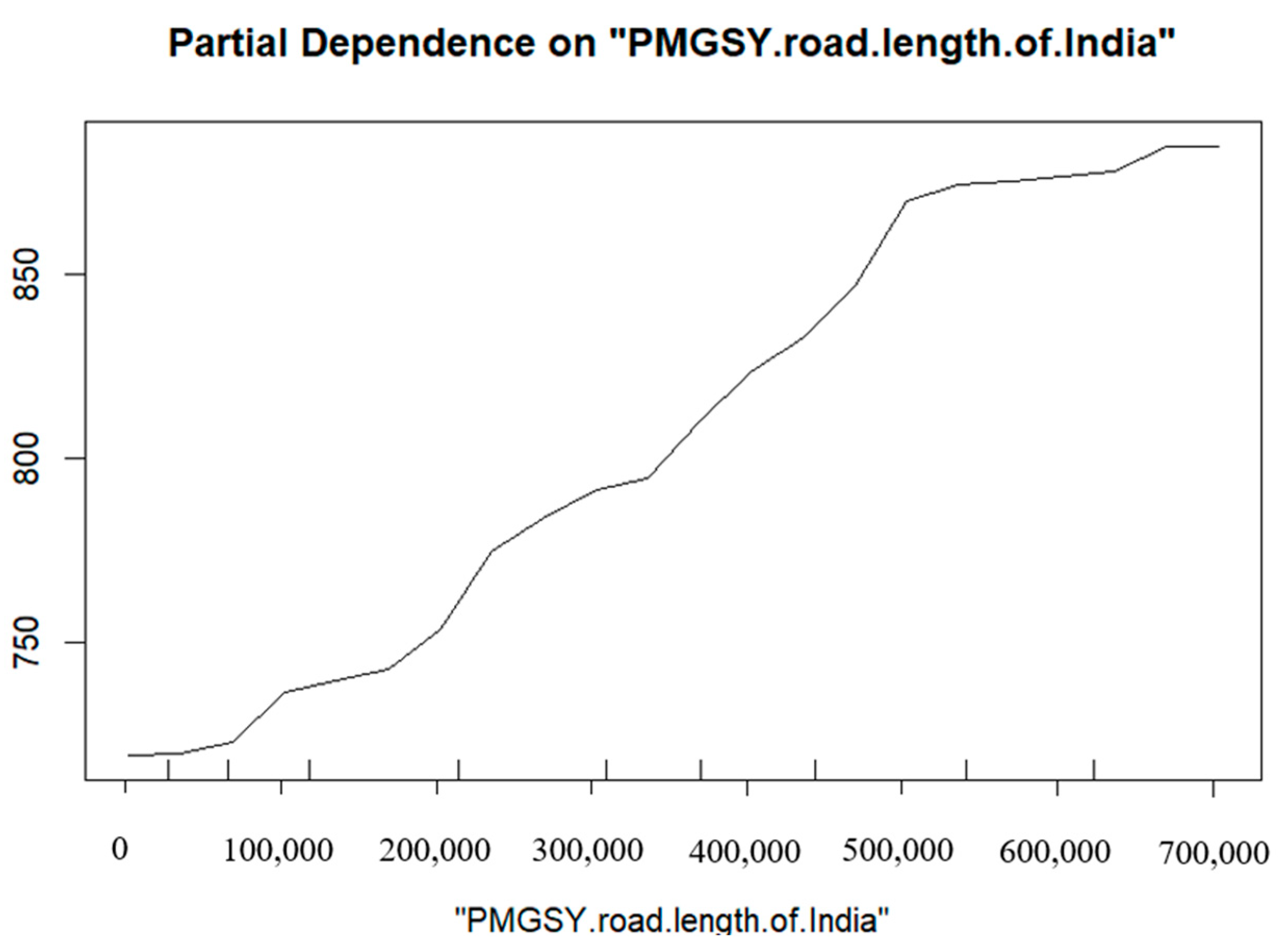
Figure 24.
Partial plot of PMGSY road length and fixed investment. Unit: kilometer; million USD.

Figure 25.
Partial plot of PMGSY road length and interest rate. Unit: kilometer; percent.
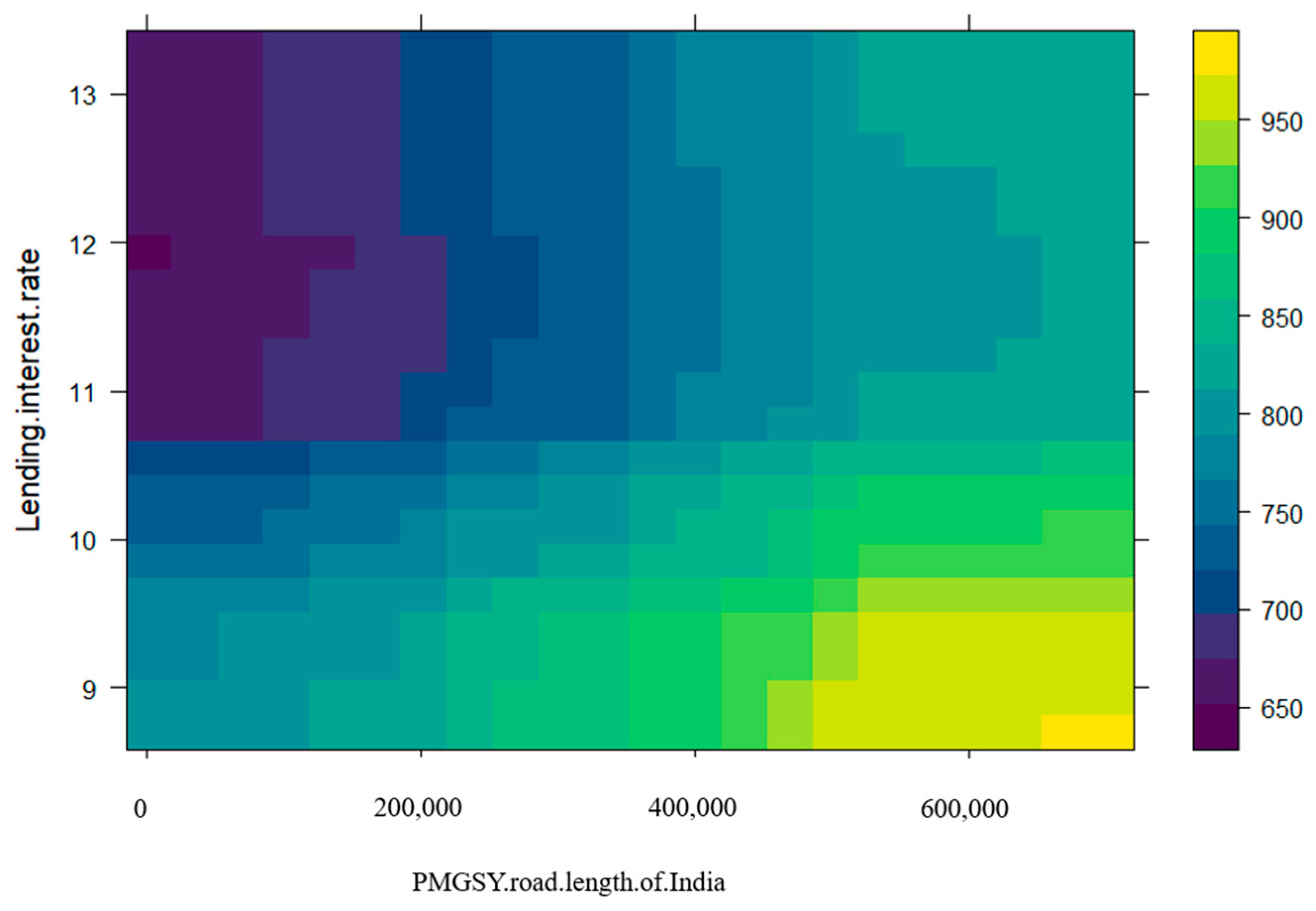
Figure 26.
Partial plot of PMGSY road length and inward direct investment. Unit: kilometer; million USD.
Figure 26.
Partial plot of PMGSY road length and inward direct investment. Unit: kilometer; million USD.
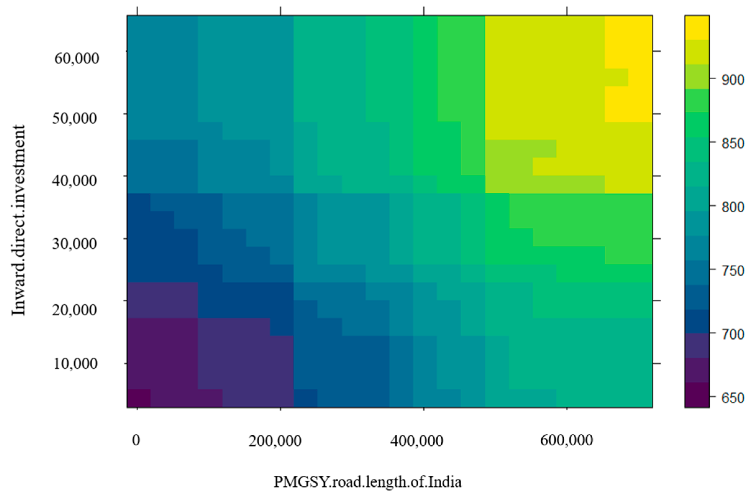
Figure 27.
Time series fitting plot for GDP development.

Table 1.
Stepwise regression of India’s data.
| Df Deviance | Deviance | AIC | |
|---|---|---|---|
| <none> | 288,127 | 285.00 | |
| Infrastructure rating | 1 | 281,029 | 286.45 |
| Inward direct investment | 1 | 325,714 | 287.69 |
| Total factor productivity growth | 1 | 329,864 | 287.97 |
| Lending interest rate | 1 | 370,585 | 290.53 |
| Real gross fixed investment | 1 | 388,203 | 291.56 |
| PMGSY road length of India | 1 | 545,594 | 299.04 |
Disclaimer/Publisher’s Note: The statements, opinions and data contained in all publications are solely those of the individual author(s) and contributor(s) and not of MDPI and/or the editor(s). MDPI and/or the editor(s) disclaim responsibility for any injury to people or property resulting from any ideas, methods, instructions or products referred to in the content. |
© 2024 by the authors. Licensee MDPI, Basel, Switzerland. This article is an open access article distributed under the terms and conditions of the Creative Commons Attribution (CC BY) license (https://creativecommons.org/licenses/by/4.0/).
Share and Cite
MDPI and ACS Style
Chen, J.; Cai, B. AIIB Investment and Economic Development of India: The Case of the Gujarat Road Project. J. Risk Financial Manag. 2024, 17, 64. https://doi.org/10.3390/jrfm17020064
AMA Style
Chen J, Cai B. AIIB Investment and Economic Development of India: The Case of the Gujarat Road Project. Journal of Risk and Financial Management. 2024; 17(2):64. https://doi.org/10.3390/jrfm17020064
Chicago/Turabian StyleChen, Jinxi, and Bowen Cai. 2024. "AIIB Investment and Economic Development of India: The Case of the Gujarat Road Project" Journal of Risk and Financial Management 17, no. 2: 64. https://doi.org/10.3390/jrfm17020064