DAO Dynamics: Treasury and Market Cap Interaction

Abstract

This study examines the dynamics between treasury and market capitalization in two Decentralized Autonomous Organization (DAO) projects: OlympusDAO and KlimaDAO. This research examines the relationship between market capitalization and treasuries in these projects using vector autoregression (VAR), Granger causality, and Vector Error Correction models (VECM), incorporating an exogenous variable to account for the comovement of decentralized finance assets. Additionally, a Generalized Autoregressive Conditional Heteroskedasticity (GARCH) model is employed to assess the impact of carbon offset tokens on KlimaDAO’s market capitalization returns’ conditional variance. The findings suggest a connection between market capitalization and treasuries in the analyzed projects, underscoring the importance of the treasury and carbon offset tokens in impacting a DAO’s market capitalization and variance. Additionally, the results suggest significant implications for predictive modeling, highlighting the distinct behaviors observed in OlympusDAO and KlimaDAO. Investors and policymakers can leverage these results to refine investment strategies and adjust treasury allocation strategies to align with market trends. Furthermore, this study addresses the importance of responsible investing, advocating for including sustainable investment assets alongside a foundational framework for informed investment decisions and future studies in the field, offering novel insights into decentralized finance dynamics and tokenized assets’ role within the crypto-asset ecosystem.

1. Introduction

Effectively managing a community’s assets on the blockchain can be transparent, mainly when the community oversees its assets and introduces its token. This study provides evidence of the relationship between the community’s assets and the overall value of its issued tokens. The findings of this research hold the potential to significantly augment decision-making processes and strategic planning within the blockchain and cryptocurrency domain by underscoring the pivotal role played by a DAO’s treasury. As such, comprehensively evaluating the composition, management, and growth trajectory of a DAO’s treasury is essential in accurately assessing the viability and potential success of a DAO project. Moreover, identifying the correlation between a DAO’s treasury and its market capitalization provides valuable insights for investors, stakeholders, and project evaluators, enabling them to proceed with informed decisions and effectively allocate resources in the ever-evolving decentralized finance landscape.

Decentralization, transparency, and security are foundational principles in the blockchain domain. The evolution of blockchain technology has led to the creation of DAOs, empowering communities to decide on their operations collaboratively. The concept of a DAO is incorporated in the Ethereum whitepaper (Buterin 2014), where it is mentioned to be a smart contract that contains the funds and the rules of an organization whose members have the right to allocate these assets and modify the rules that govern it, allowing for the automation of certain processes that are defined in the smart contract. A DAO can issue its token and form an ecosystem where each token provides voting rights to its holder, excluding its marketplace value. Consequently, every holder impacts the DAO’s decision making through transparent voting processes, aligning with the fundamental tenets of decentralization in the blockchain.

Decentralized finance (DeFi) is rooted in traditional financial activities on the blockchain, like lending and trading without intermediaries. With the advent of DeFi 2.0, the field incorporated the idea of a DAO making decisions regarding a project’s liquidity within the protocol. An advancement was implemented by OlympusDAO in 2021, and their paradigm led to the creation of numerous similar projects, where the community of the protocol owned and decided its treasury and its diversification (Spinoglio 2022). Additionally, token holders from the DAO possess voting privileges, which play a pivotal role in shaping the community’s future choices, as observed in the KlimaDAO project (Freni et al. 2022). Finally, in DeFi projects, the tokenized assets owned by the protocol are held in the “treasury,” which is in the form of smart contracts, and the use of a treasury’s funds is decided through a voting process (Bhambhwani 2023). The purpose of the treasury in OlympusDAO is to support the DAO’s issued token liquidity (Olympus Docs n.d.).

The KlimaDAO project, while related to OlympusDAO as a DeFi 2.0 project, is a pioneer in the Regenerative Finance (ReFi) sector (Baim 2023) and is referenced as such by other authors as well (Bordeleau and Casemajor 2023). ReFi is a term connected to DeFi, as they both use the same tools, but ReFi is focused on services linked to regenerative economics (Schletz et al. 2023). KlimaDAO, a project with the goal of combatting climate change (Oguntegbe et al. 2023), aims to establish a carbon-based cryptocurrency, participating in the voluntary carbon market using Web3 technology, where Web3 is a broader concept of the evolution of the internet, where the data is stored and distributed through a decentralized network, utilizing the transparency, inclusivity, and immutability that blockchain technology allows, and the processes can be automated using smart contracts (Murray et al. 2023). Each KlimaDAO token’s (KLIMA) value is alleged to be backed by one carbon ton from tokens issued by Moss Earth, Toucan protocol, and C3 protocols, whose tokens are backed by carbon offset credits from carbon registries like Verra and Gold Standard (KlimaDAO 2022). The treasury of KlimaDAO consists of tokens that include carbon offset, such as Base Carbon Ton (BCT), and non-carbon offset tokens, such as stablecoins. However, KlimaDAO token holders benefit from the increase in the KlimaDAO token price, considering that token ownership is linked to financial rewards derived from the reserves of the KlimaDAO treasury (Dobrajska 2023), rendering the treasury a vital aspect of the project.

However, tokenizing carbon credits is a controversial subject that led to the subsequent announcements by Verra (Verra 2021, 2022, 2023), where it declared no responsibility and involvement for such activities. Therefore, Verra conducted a multi-week public consultation regarding the approach towards the activities associating tokens with instruments issued by Verra along with regulatory-associated concerns. Additionally, Babel et al. (2022) cite KlimaDAO when focusing on the transparency issues of voluntary carbon offsets by highlighting KlimaDAO as a market facilitating investment in projects targeting carbon dioxide consumption while integrating blockchain technology aids in tracking these offsets, thereby mitigating the risk of duplicate spending.

KlimaDAO and OlympusDAO represent significant advancements in decentralized finance, particularly integrating decentralized autonomous organizations into their operational frameworks. One fundamental similarity between the two projects is their reliance on DAO governance models, where community members hold voting privileges to influence protocol decisions and manage the project’s treasury. Both projects prioritize liquidity management within their respective ecosystems, leveraging their treasuries to support token liquidity and ensure ecosystem stability.

However, there are notable differences between KlimaDAO and OlympusDAO regarding their primary objectives and focus areas. As a pioneer in the DeFi 2.0 space, OlympusDAO emphasizes the stability of its native token “OHM”, backed by assets such as “DAI”, which is a stablecoin issued by MakerDAO and is backed by collateral (Maker Team 2017), and wrapped Ether (wETH) (Rossello 2024), and the creation of a robust reserve currency. In contrast, KlimaDAO distinguishes itself as a pioneer in the emerging Regenerative Finance field, specifically focusing on leveraging blockchain technology to address environmental concerns. KlimaDAO aims to establish a carbon-based cryptocurrency backed by carbon offset credits, contributing to the voluntary carbon market and promoting sustainability initiatives. This divergence in objectives reflects the diverse applications and use cases within the broader DeFi ecosystem, showcasing the versatility and innovation inherent in decentralized finance projects.

Hence, our study exclusively centers on OlympusDAO and KlimaDAO for several reasons. Firstly, we aim to compare two projects with similar smart contract characteristics, given that KlimaDAO is a fork of OlympusDAO. Secondly, we emphasize the significance of these projects: OlympusDAO as a pioneer in the DeFi 2.0 sector and KlimaDAO as a pioneer in the ReFi sector, encompassing both DeFi 2.0 and ReFi. Lastly, the growing number of scholarly articles on OlympusDAO and KlimaDAO indicates ongoing interest in these projects.

While the significance of the examined projects has been acknowledged in the existing literature, there remains a gap in understanding the importance of their treasury management from an econometric perspective. Specifically, there is a lack of studies that econometrically analyze the relationship between these projects and their treasuries while considering external factors such as the comovement of similar assets. Furthermore, no previous research has explored how specific tokens might impact the market capitalization of a DAO, initiating an inquiry into the potential influence of carbon offsets within a diversified portfolio, potentially represented by tokenized carbon credits. This research aims to bridge these gaps by providing empirical evidence on the interplay between project significance, treasury management, and token dynamics within DAOs.

The current study examines whether a two-way relationship between the treasuries of OlympusDAO and KlimaDAO and their market capitalization exists by employing a Vector Autoregression model with exogenous variables, further cointegration tests, and two Vector Error Correction models regarding the returns of the market caps of the examined DAOs, and Granger causality tests. Moreover, it is within the scope of our analysis to ascertain whether carbon offset tokens can validate the concept of DAO-issued tokens possessing intrinsic value via tokenized carbon credits, potentially raising regulatory considerations. Therefore, we aim to evaluate the impact of carbon offset tokens on the conditional variance within a GARCH model to tackle issues of conditional heteroskedasticity in the time series, focusing specifically on the case study of KlimaDAO.

The structure of this study is as follows: Section 2 details the literature review, Section 3 explains the methodology, Section 4 presents the results, Section 5 details the discussion, and Section 6 encapsulates this study’s conclusions.

2. Literature Review

Song et al. (2023), while documenting the mechanism behind OlympusDAO, highlighted the importance of the OlympusDAO token, as well as the treasury mechanism of the project. They explained in detail the staking and bonding mechanisms of the project, which are the main elements of increasing the treasury that supports the DAO’s token. The bonding mechanism allows potential investors to buy the OlympusDAO token at a discount, resulting in the subsequent cash flows being directed to the DAO’s treasury, and the staking mechanism gives an incentive to the DAO token holders to deposit their tokens in the treasury and obtain interest, in DAO tokens, for their deposit. Subsequently, the treasury assets are used to back the DAO’s token, whose price should not fall under one dollar. When using the treasury funds, the DAO makes such decisions through a voting mechanism with transparent and secure procedures. Chitra et al. (2022) find the role of the treasury to be that of an indirect “insurance fund”. The concept of a protocol owning its liquidity was coined initially by OlympusDAO (Pupyshev et al. 2022). The OlympusDAO token is alleged to represent its underlying collateral (Ante et al. 2023); however, Guo et al. (2024) state that the staking system employed by OlympusDAO encouraged users to stake their tokens by offering high rewards, but this system led to high inflation that resulted in the token’s decreasing value. Mislavsky (2024) also refers to the high yields of OlympusDAO tokens that helped the project initially gain public exposure and market capitalization, but inevitably, these yields decreased along with its market capitalization.

Jirásek (2023) studied the organizational model of KlimaDAO, inspired by OlympusDAO, and characterized KlimaDAO as a notable example among other DAOs. Jirásek acknowledged KlimaDAO’s commitment to its mission, which led to the acquisition of around 4% of all voluntary carbon market credits by October 2022. However, Foss and Xu (2023), while recognizing Jirásek’s contributions, diverge from the author’s conclusions regarding KlimaDAO’s business model, citing the volatility of KlimaDAO tokens but refraining from analyzing this volatility. He and Puranam (2023) also note that KlimaDAO presents a unique organizational structure compared to similar entities; however, they notice weaknesses in KlimaDAO’s organizational structure, including founder anonymity and legal ambiguity, alongside the broader challenges DAOs face. Hence, founder anonymity does not deter an individual from taking legal action against the alleged founders of a DAO project, as in the case of OlympusDAO (Ghodoosi 2022).

Sicilia et al. (2022) highlighted the similarities between KlimaDAO and the OlympusDAO protocol, underscoring the depth of inspiration, where both platforms center around establishing a treasury via bonding and staking mechanisms within a game theoretic framework aimed at price stabilization. In particular, staking in KlimaDAO mirrors OlympusDAO’s strategy, incentivizing long-term token holding to garner compounded rewards and exposure to carbon price fluctuations. Similarly, bonding in KlimaDAO echoes OlympusDAO’s approach, enabling discounted token acquisition over a vesting period, with pricing dynamics responding sensitively to demand fluctuations. Sicilia et al. also denoted the significance of the KlimaDAO project, exploring the mechanism behind the carbon offset tokens. Finally, the authors acknowledged the complexity of this mechanism and suggested that future works could be focused on assessing the impact of the tokenized carbon offsets in DeFi. Sorensen (2023) added that KlimaDAO aims to stimulate demand for carbon credits, establishing a “carbon economy”, wherein the currency is backed by carbon, and the total cost of carbon is integrated into each transaction.

In their endeavor to develop a scale for assessing the readiness of blockchain applications for carbon markets, Sipthorpe et al. (2022) categorize KlimaDAO as a “fully competitive” project, the sole DAO project at the highest tier of their scale. Nonetheless, Sipthorpe et al. recognize the market’s immaturity and the challenges associated with these endeavors, mainly due to the lack of pertinent regulations that might deter potential investors from participating in this domain.

Ziegler and Welpe (2022) highlighted the treasury as a crucial attribute of DAOs, while Metelski and Sobieraj (2022) suggested the potential for further investigation into the connection between a DeFi project’s treasury and its valuation, leading to a more precise assessment of a DeFi’s value, taking its treasury assets into account.

Nowak (2022) addressed the issue of carbon credit tokenization and noted its innovative significance for the carbon offset markets; Nowak also cites KlimaDAO and the tokens it creates in this context. Moreover, Armisen et al. (2024) analyze the disparity in user behavior between expert and regular users in utilizing carbon offsets within KlimaDAO based on blockchain data, and they observe differing choices made by these user categories in selecting carbon offsets.

In brief, our examination of the literature did not uncover any relevant studies concerning the econometric evaluation of either the treasury or the market capitalization of a DAO and their reciprocal influence on each other, while analyzing the market capitalization of the projects could be a better approach instead of analyzing the prices of the tokens, because of the inflation mechanism. Additionally, while several articles discuss the importance of KlimaDAO’s organizational structure and economic model, there has been little research on how the tokenized carbon credits in its treasury influence the project’s market capitalization or analyze the volatility of the project’s tokens. Hence, this study adds to the body of literature by elucidating the interconnections between two significant DAOs, their respective treasuries, and the potential financial impact of carbon tokens.

3. Methodology

3.1. Data Collection and Filtering

The analyzed period in the daily data is between 27 October 2021 and 16 September 2023. The period analyzed was selected to encompass all variables under examination, guided by the data available during the study. Given that KlimaDAO was launched later than OlympusDAO, we aimed for uniformity in the examined variables, necessitating a period inclusive of all relevant data. The OlympusDAO and KlimaDAO treasury data were acquired from Defillama (n.d.) (accessed on 8 November 2023), and market capitalization data were sourced from Coingecko (n.d.). The data regarding the treasuries of the DAOs are denominated in US dollars (USD). Moreover, we obtained the time series for the “Top 100 DeFi Coins by Market Capitalization” from Coingecko to account for the comovement of asset prices, representing the aggregate market capitalization of the top 100 DeFi coins, as determined by Coingecko. The variables that are examined in this analysis are presented in

Table 1. Examined variables.

Variable	Meaning
Olympus_MC	Natural logarithm of the Market Cap of OlympusDAO
Klima_MC	Natural logarithm of the Market Cap of KlimaDAO
Olympus_Tr	Natural logarithm of the Treasury of OlympusDAO
Klima_Tr	Natural logarithm of the Treasury of KlimaDAO
Defi_MC	Natural logarithm of the Market Cap of the Top 100 DeFi Coins by Market Capitalization by Coingecko
KCT	Natural logarithm of the KlimaDAO Carbon Tokens total value
r_Olympus_MC	Returns of the Market Cap of OlympusDAO
r_Klima_MC	Returns of the Market Cap of KlimaDAO
r_Olympus_Tr	Returns of the Treasury of OlympusDAO
r_Klima_Tr	Returns of the Treasury of KlimaDAO
r_Defi_MC	Returns of the Market Cap of the Top 100 DeFi Coins by Market Capitalization by Coingecko
r_KCT	Returns of the KlimaDAO Carbon Tokens’ total value

.

The variables chosen for analysis comprise the natural logarithm of the market capitalizations and treasuries of the projects under examination, along with the market capitalization of the leading DeFi coins, serving as a proxy for the comovement of similar assets and the total value of the KlimaDAO carbon tokens alongside their respective returns. This transformation was implemented to assess stationarity, present pertinent findings, and calculate returns where stationarity was not observed, as demonstrated in the subsequent results. We utilized market capitalization (MC) variables because the token price alone may not accurately reflect the total project value, as in crypto assets token supply is often subject to dynamic changes, a characteristic observed in the specific projects under scrutiny. The OlympusDAO market capitalization variable was selected for its status as a pioneer in DeFi 2.0, while the KlimaDAO market capitalization was chosen for its prominence in the ReFi sector. The KlimaDAO carbon tokens (KCT) variable is essential because it represents the total value of the carbon offset tokens in KlimaDAO.

In the context of our study, the variables are denoted with the suffix “_d” to represent daily measurements, and the monthly averages from the daily values are denoted with the suffix “_m” to indicate their monthly aggregation.

The OlympusDAO treasury data encompassed tokens in the DAO’s treasury across Ethereum, Polygon, Arbitrum, and Fantom blockchains, along with their corresponding USD values. Similarly, the KlimaDAO treasury comprised all the tokens under the DAO’s management. The formula for the treasury is presented in Equation (1).

$${Treasury}_{DAO, t}=\sum _{i=1}^p{CA}_{i,t}$$

(1)

In Equation (1), the treasury of a DAO consists of the total sum of the crypto assets (CAs) that are included in the respective treasury smart contracts managed by the DAO at time t.

Next, to analyze further the effects of the carbon offset treasury in KlimaDAO, we identify KCT, which consists of the tokens that KlimaDAO explicitly characterizes as “carbon tokens” (CTs) (KlimaDAO 2022), which are BCT, NCT, MCO2, UBO, NBO, and in the KCT, we include any liquidity pool token containing these assets, all of which are held in the KlimaDAO treasury, resulting in Equation (2).

$${KCT}_t=\sum _{i=1}^p{CT}_{i,t}$$

(2)

In Equation (2), at the time t, the KCT is the sum of every CT.

3.2. VAR Model

A Vector Autoregressive (VAR) model is used to analyze the interdependence of system variables. This model assumes that every variable in the system is expressed as a function of its lags and the lags of all the other variables in the system. By estimating the parameters of the VAR model, we can gain insights into the dynamic relationships among the different variables and make predictions about their future values.

Our model incorporates r_Klima_MC_m_t, r_Olympus_MC_m_t, r_Klima_Tr_m_t, and r_Olympus_Tr_m_t as endogenous variables, and r_Defi_MC_m_t as an exogenous variable. The optimal lag length for our model was determined to be one after analyzing the information criteria. Based on our best estimation, the VAR(1) model is presented in Equation (3).

$$Y_t=A_1{Y}_{t-1}+B{X}_t+{\epsilon }_t$$

(3)

Let Y_t be the vector of endogenous variables at time t, A₁ as the matrix containing the lag coefficients, Y_t−1 as the lagged vector of endogenous variables, B as the matrix of coefficients for the exogenous variables, X_t as the vector of exogenous variables at time t, and ε_t as the vector of error terms. According to the above, the model may be written as Equation (4):

$$\begin{array}{c}{Y}_t=\left[\begin{array}{c}{r\_Klima\_MC\_m}_t\\ {r\_Olympus\_MC\_m}_t\\ {r\_Klima\_Tr\_m}_t\\ { r\_Olympus\_Tr\_m}_t\end{array}\right]\\ =\left[\begin{array}{c}{a}_1\\ a_2\\ a_3\\ a_4\end{array}\right]+\left[\begin{array}{c}\begin{array}{ccc}{\beta }_{\mathrm{1,1}}& {\beta }_{\mathrm{1,2}}& \begin{array}{cc}{\beta }_{\mathrm{1,3}}& {\beta }_{\mathrm{1,4}}\end{array}\end{array}\\ \begin{array}{ccc}{\beta }_{\mathrm{2,1}}& {\beta }_{\mathrm{2,2}}& \begin{array}{cc}{\beta }_{\mathrm{2,3}}& {\beta }_{\mathrm{2,4}}\end{array}\end{array}\\ \begin{array}{ccc}{\beta }_{\mathrm{3,1}}& {\beta }_{\mathrm{3,2}}& \begin{array}{cc}{\beta }_{\mathrm{3,3}}& {\beta }_{\mathrm{3,4}}\end{array}\end{array}\\ \begin{array}{ccc}{\beta }_{\mathrm{4,1}}& {\beta }_{\mathrm{4,2}}& \begin{array}{cc}{\beta }_{\mathrm{4,3}}& {\beta }_{\mathrm{4,4}}\end{array}\end{array}\end{array}\right]+\left[\begin{array}{c}{r\_Klima\_MC\_m}_{t-1}\\ {r\_Olympus\_MC\_m}_{t-1}\\ {r\_Klima\_Tr\_m}_{t-1}\\ { r\_Olympus\_Tr\_m}_{t-1}\end{array}\right]\\ +\left[\begin{array}{c}{\gamma }_1\\ {\gamma }_2\\ {\gamma }_3\\ {\gamma }_4\end{array}\right]{r\_DeFi\_MC\_m }_t+\left[\begin{array}{c}{\epsilon }_{1,t}\\ {\epsilon }_{2,t}\\ {\epsilon }_{3,t}\\ {\epsilon }_{4,t}\end{array}\right]\end{array}$$

(4)

3.3. Cointegration Tests and VECM

The Johansen cointegration test (Johansen 1991) has been utilized to investigate a long-term relationship among the variables in our model. This test aims to determine whether cointegrating vectors exist in the spectrum of a Vector Autoregression (VAR) model. Through this examination, we have determined if a cointegration equation exists, indicating a long-term relationship between the variables under consideration. The null hypothesis in this test assumes the absence of a cointegration equation. Therefore, the Johansen cointegration test results clearly understand the presence or absence of any underlying relationships between the variables in our model.

Finally, we incorporated a Vector Error Correction model (Engle and Granger 1987) for r_Olympus_MC and r_Klima_MC to examine the short-run deviations from the long-run equilibrium. This dynamic adjustment captures the short-term dynamics and helps understand how the system responds to shocks.

3.4. Granger Causality Test

In order to make accurate predictions using time series data, it is crucial to determine whether any variables can be used as predictors for one another. Causality plays a critical role in time series analysis, as it measures the extent to which one variable’s values can be used to forecast another variable’s values. By understanding causality, we can gain more insights into future outcomes of a time series based on the values of contiguous time series over time.

Granger causality, introduced by Granger in 1969, is a statistical technique that uses Vector Autoregressive Models to determine the direction and strength of causality between two time series. Although VAR modeling helps identify the relationships and dependencies among variables, it cannot establish causality. The Granger causality test can be used to determine whether past values of a variable can provide information about future values of another variable and, therefore, establish causality.

In order to apply this method, the variables must be stationary or cointegrated. A VAR model of order p can be defined as follows in Equation (5):

$$\begin{array}{c}{y}_t={\beta }_{\mathrm{1,0}}+{\displaystyle \sum _{i=1}^p} {\beta }_{1,i}{y}_{t-i}+{\displaystyle \sum _{j=1}^p} {\beta }_{1,p+j}{x}_{t-i}+e_{1t}\\ x_t={\beta }_{\mathrm{2,0}}+{\displaystyle \sum _{i=1}^p} {\beta }_{2,i}{y}_{t-i}+{\displaystyle \sum _{j=1}^p} {\beta }_{2,p+j}{x}_{t-i}+e_{2t}\end{array}$$

(5)

For the sake of illustration, we use variables y_t and x_t. The order of the Vector Autoregression (VAR) model refers to the number of lags required to validate the hypothesis that each error term is white noise (Shojaie and Fox 2022). We can say that “y_t Granger causes x_t” if the past values of y_t are statistically significant. To examine if x_t Granger causes y_t, the testing process needs to be repeated in the opposite direction.

In our analysis, we will investigate whether the returns of OlympusDAO and KlimaDAO market capitalization and their treasuries Granger cause each other. In order to address the comovement of asset prices, we used the r_Defi_MC as a proxy.

3.5. GARCH Analysis

Based on our analysis, we have determined that a GARCH(1,1) model is the most appropriate. The conditional mean equation is a fundamental component in the statistical modeling of the expected or mean value of a financial time series. The conditional mean is presented in Equation (6).

$$\begin{gathered} {r\_Klima\_MC\_d}_t=\mu +{{\phi }_{1}r\_Klima\_MC\_d}_{t-1}+{{\xi }_{1}r\_Defi\_MC\_d}_t \\ +{{\xi }_{2}r\_Defi\_MC\_d}_{t-1}+{\epsilon }_t \end{gathered}$$

(6)

where μ is the constant, and r_Klima_MC and r_Defi_MC are the logarithmic returns of KlimaDAO market cap and the “Top 100 DeFi Coins by Market Capitalization”, respectively, to address the issues of stationarity, as the variables are I(1) series according to the augmented Dickey–Fuller (ADF) test and Kwiatkowski–Phillips–Schmidt–Shin (KPSS) tests.

For this analysis, we shall employ the Generalized Autoregressive Conditional Heteroskedasticity model, an indispensable tool for comprehending the intricacies of volatility in financial markets (Bollerslev 1986). Our primary emphasis will be on the results of the GARCH analysis, which will furnish us with a granular comprehension of the dynamics of the conditional variance. The conditional variance equation is a pivotal facet of GARCH modeling, encapsulating insights into the volatility or dispersion evident in the financial series. The conditional variance equation of a GARCH(p, q) model, where p stands for the number of lagged conditional variances, and q denotes the number of lagged squared residuals, can be expressed as follows in Equation (7).

$${\sigma }_t^2=\omega +\sum _{i=1}^p{a}_i{{\epsilon }^2}_{t-i}+\sum _{j=1}^q{\beta }_j{{\sigma }^2}_{t-j}$$

(7)

We denote by ω the constant term representing the long-term average level of volatility, used as a baseline volatility measure in the absence of any shocks, α_i stands for the ARCH coefficients applied to capture the impact of past squared residuals on the current conditional variance. ${\epsilon }_{t-i}^2$ are the squared residuals at time t − i, representing the unexpected shocks or errors in the model. By β_j, we define the GARCH coefficients to capture the impact of past conditional variances on the current conditional variance. As ${\sigma }_{t-j}^2,$ we define the lagged conditional variances representing the past volatility of the model.

Greater values of α_i indicate a more persistent effect of past shocks on volatility. In comparison, greater values of β_j indicate a more persistent effect of past volatility on the current volatility.

Our findings suggest that we may model the conditional variance using a GARCH model of the first order for the ARCH effects, the first order for the GARCH, and the first order for leverage effects, plus the returns of the KlimaDAO Carbon Tokens as r_KCT as an exogenous variable in the conditional variance equation. The GARCH equation is now transformed as follows (8):

$${\sigma }_t^2=\omega +a_1{{\epsilon }^2}_{t-1}+{\beta }_1{{\sigma }^2}_{t-1}+{{\psi }_{1}r\_KCT\_d}_t$$

(8)

3.6. Utilized Software

“Grammarly 6.8.263” (Grammarly: Free AI Writing Assistance n.d.) was used for grammar and language correction, while “ChatGPT 3.5” (ChatGPT n.d.) helped in expressing the content and refined the English language where necessary. Additionally, “Zotero 6.0.36” (Zotero n.d.) was utilized to index pertinent references for the paper, noted in this manuscript’s “Acknowledgments” section.

4. Results

4.1. Examined Variables

Table 2. Stationarity tests.

Variable	ADF		KPSS
	Statistic	p-Value	Statistic	p-Value
Olympus_MC	−3.73	0.00 ***	0.64	0.01 ***
Klima_MC	−2.94	0.04 **	0.69	0.01 ***
Olympus_Tr	−2.61	0.09 *	0.15	0.04 **
Klima_Tr	0.15	0.97	0.39	0.01 ***
Defi_MC	−1.72	0.42	2.00	0.01 ***
r_Olympus_MC	−22.43	0.00 ***	0.11	0.10
r_Klima_MC	−11.03	0.00 ***	0.12	0.10
r_Olympus_Tr	−12.28	0.00 ***	0.04	0.10
r_Klima_Tr	−11.55	0.00 ***	0.08	0.10
KCT_d	−2.69	0.08 *	0.68	0.01 ***
r_KCT_d	−15.56	0.00 ***	0.08	0.10
r_Defi_MC	−25.19	0.00 ***	0.18	0.10
Olympus_MC_m	1.33	0.00 ***	0.16	0.04 **
Klima_MC_m	−2.66	0.00 ***	0.17	0.03 **
Olympus_Tr_m	−0.79	0.80	0.41	0.05 **
Klima_Tr_m	0.23	0.96	1.87	0.01 ***
Defi_MC_m	−1.94	0.31	0.35	0.10
r_Olympus_MC_m	−3.64	0.01 ***	0.34	0.10
r_Olympus_Tr_m	−5.56	0.00 ***	0.05	0.10
r_Klima_MC_m	−3.28	0.03 **	0.37	0.10
r_Klima_Tr_m	1.13	0.00 ***	0.088	0.10
r_Defi_MC_m	−5.16	0.00 ***	0.12	0.10

Note: * indicates significance at the 10% level, ** at the 5% level, and *** at the 1% level.

presents the results regarding the stationarity tests and indicates the selection of the final variables to be examined in the subsequent analysis.

In Table 2, for our analysis, we selected the natural logarithmic values of the examined variables and their respective returns. We observe that in all cases where the variables are in their logarithmic form, the KPSS test for stationarity is rejected when testing for trend stationarity, even if the ADF test null hypothesis for the existence of a unit root is rejected in two cases. Therefore, to ensure that no unit root exists in our time series, we calculate the returns of the variables. In the returns of the variables, we observe that the null hypothesis of a unit root regarding the ADF test is rejected in all cases, and the null hypothesis of trend stationarity regarding the KPSS test is not rejected in all cases. Subsequently, in our analysis, we will use the logarithmic returns of the variables. The descriptive statistics of the examined variables are presented in

Table 3. Descriptive statistics of the examined variables.

Variable	Statistic
	Mean	Standard Deviation	Range	Max	Min	Median	Skewness	Kurtosis	Jarque–Bera (JB)	Jarque–Bera p-Value
r_Klima_MC_d	−0.007	0.061	0.713	0.267	−0.447	−0.004	−0.945	11.079	1978.948	0.000
r_KCT_d	−0.003	0.054	0.680	0.327	−0.354	−0.233	−0.021	13.338	3072.755	0.000
r_Defi_MC_d	−0.002	0.036	0.501	0.121	−0.380	0.001	−2.347	23.369	12,561.000	0.000
r_Olympus_MC_m	−0.004	0.010	0.049	0.006	−0.043	0.000	−2.664	10.697	87.623	0.000
r_Olympus_Tr_m	−0.001	0.009	0.051	0.018	−0.033	0.000	−1.571	9.524	52.435	0.000
r_Klima_MC_m	−0.009	0.017	0.078	0.017	−0.061	−0.006	−1.328	5.247	12.104	0.002
r_Klima_Tr_m	−0.003	0.010	0.056	0.031	−0.025	−0.005	1.333	6.696	20.775	0.000
r_Defi_MC_m	−0.002	0.007	0.035	0.010	−0.025	−0.001	−1.115	5.454	10.997	0.004

Note: all daily (“_d”) variables have 690 observations, and all monthly (“_m”) variables have 24 observations each.

.

Table 3 shows that all variables’ skewness and kurtosis values indicate asymmetry and peakedness in their distributions. Subsequently, the Jarque–Bera statistics, with p-values close to zero, reject the null hypothesis of a normal distribution for each variable. Figure 1 presents the box plots of the examined daily value variables.

As depicted in Figure 1, the daily box plot values indicate that the medians are approximately zero, with consistent interquartile ranges and whisker sizes across all instances. However, a notable difference emerges: for r_Klima_MC_d and r_KCT_d, the number of outlier values is relatively similar and more abundant compared to r_Defi_MC_d, where fewer outliers are observed. Figure 2 presents the box plots of the examined monthly value variables.

As depicted in Figure 2, the median values of the variables under examination hover around zero or slightly negative values close to zero. A comparative analysis of the variables reveals that r_Klima_MC_m exhibits somewhat longer whiskers than the others, which maintain similar whisker ranges. The interquartile ranges vary among the variables, with the upper quartiles of r_Olympus_Tr_m and r_Olympus_MC_m being relatively small. Regarding outliers, r_Defi_MC_m displays a higher count than the other variables, while r_Olympus_MC_m exhibits no positive value outliers. The remaining variables show outlier variation ranging from three to four outliers per analyzed variable, with values ranging from 0.02 to −0.06.

4.2. VAR Results

Table 4. VAR estimation results.

Variable	Dependent Variable
	r_Klima_MC_m	r_Olympus_MC_m	r_Klima_Tr_m	r_Olympus_Tr_m
r_Klima_MC_m(−1)	0.143	0.318	−0.339	0.170
	(0.140)	(0.094)	(0.169)	(0.114)
	[1.023]	[3.382]	−[2.004]	[1.489]
r_Olympus_MC_m(−1)	0.358	−0.137	0.264	0.041
	(0.213)	(0.143)	(0.258)	(0.174)
	[1.681]	−[0.955]	[1.024]	[0.234]
r_Klima_Tr_m(−1)	−0.543	−0.605	0.196	−0.814
	(0.222)	(0.149)	(0.269)	(0.181)
	−[2.449]	−[4.055]	[0.731]	−[4.499]
r_Olympus_Tr_m(−1)	0.383	0.857	0.135	−0.057
	(0.209)	(0.140)	(0.253)	(0.170)
	[1.837]	[6.114]	[0.534]	−[0.335]
C	−0.003	−0.001	−0.003	−0.002
	(0.002)	(0.001)	(0.002)	(0.002)
	−[1.353]	−[0.977]	−[1.270]	−[1.392]
r_Defi_MC_m	1.148	0.569	0.562	−0.112
	(0.223)	(0.150)	(0.271)	(0.182)
	[5.138]	[3.789]	[2.077]	−[0.613]
R2	0.716	0.792	0.363	0.566

Note: standard errors are indicated within parentheses (), while t-statistics are denoted within square brackets [].

presents the results of the VAR estimations and the diagnostics in Appendix A in

Table A1. VAR diagnostics.

Residual Serial Correlation LM TEST
Lag	LRE Stat	d.o.f.	Prob.
1	21.982	16	0.144
2	13.678	16	0.623
VAR Residual Heteroskedasticity
Joint test
Chi-square	d.o.f.	Prob.
107.069	100	0.296
VAR Residual Normality Tests
Component	Jarque–Bera	d.o.f.	Prob.
1	0.025	2	0.988
2	0.666	2	0.717
3	1.325	2	0.516
4	3.090	2	0.213
Joint	5.106	8	0.746
Lag Length Selection Criteria
Lag	LR	AIC	SC
0	NA	−28.49	−28.09
1	50.37 *	−30.32	−29.13 *
2	23.63	−30.94	−28.95
3	12.58	−31.22 *	−28.43

Note: The asterisk (*) indicates the optimal model length based on lag selection criteria.

.

According to our findings, the lagged variable r_Klima_MC_m_t−1 significantly impacts r_Olympus_MC_m_t and r_Klima_Tr_m_t. The lagged variable r_Olympus_MC_m_t−1 does not seem statistically significant at the 5% level. Next, the lagged variable r_Klima_Tr_m_t−1 has a significant relationship with r_Klima_MC_m_t and r_Olympus_MC_m_t, just as with r_Olympus_Tr_m_t. Furthermore, the lagged variable r_Olympus_Tr_m_t−1 has a significant impact on r_Olympus_MC_m_t. Finally, the exogenous variable r_Defi_MC_m_t is statistically related to r_Klima_MC_m_t, r_Olympus_MC_m_t, and r_Klima_Tr_m_t.

4.3. Granger Causality Results

In

Table 5. Granger causality results.

Dependent Variable: r_Klima_MC_m
Excluded Variable	Chi-square Statistic	Degrees of Freedom	Prob.
r_Olympus_MC_m	2.825	1	0.093 *
r_Klima_Tr_m	5.996	1	0.014 **
r_Olympus_Tr_m	3.374	1	0.066 *
All	14.983	3	0.002 ***
Dependent Variable: r_Olympus_MC_m
Excluded Variable	Chi-square Statistic	Degrees of Freedom	Prob.
r_Klima_MC_m	11.440	1	0.001 ***
r_Klima_Tr_m	16.440	1	0.000 ***
r_Olympus_Tr_m	37.386	1	0.000 ***
All	49.610	3	0.000 ***
Dependent Variable: r_Klima_Tr_m
Excluded Variable	Chi-square Statistic	Degrees of Freedom	Prob.
r_Klima_MC_m	4.016	1	0.045 **
r_Olympus_MC_m	1.049	1	0.306
r_Olympus_Tr_m	0.286	1	0.593
All	5.211	3	0.157
Dependent Variable: r_Olympus_Tr_m
Excluded Variable	Chi-square Statistic	Degrees of Freedom	Prob.
r_Klima_MC_m	2.218	1	0.136
r_Olympus_MC_m	0.055	1	0.815
r_Klima_Tr_m	20.239	1	0.000 ***
All	21.535	3	0.000 ***

Note: asterisks ***, **, and * represent significance at the 1%, 5%, and 10% levels, respectively.

, we present the Granger causality test results.

As shown in Table 5, there is evidence of Granger causality from r_Klima_Tr_m to r_Klima_MC_m. Next, there is strong evidence of Granger causality from r_Klima_MC_m, r_Klima_Tr_m, and r_Olympus_Tr_m to r_Olympus_MC_m, with the null hypothesis rejected at the 1% level for all cases. Furthermore, the null hypothesis of no Granger causality from r_Klima_MC_m to r_Klima_Tr_m is rejected at the 5% level. Finally, there is strong evidence of Granger causality from r_Klima_Tr_m to r_Olympus_Tr_m.

4.4. VECM and Cointegration Results

After applying the Trace and Maximum Likelihood criteria, as shown in

Table 6. Unrestricted Cointegration Rank Test (Trace).

Hypothesized Number of Cointegrating Equations	Eigenvalue	Trace Statistic	0.05 Critical Value	Probability
None	0.951	129.577	47.856	0.000 ***
At most 1	0.756	63.120	29.797	0.000 ***
At most 2	0.661	32.084	15.495	0.000 ***
At most 3	0.315	8.311	3.841	0.004 ***

Note: asterisks “***” denote rejection of the null hypothesis at the 1% level.

, we have rejected the null hypothesis, indicating that long-term relationships exist among the variables in question. These findings mean that any external shocks will not affect the long-run stability of the model, as the returns will eventually converge over time.

Initially, our attention is directed towards establishing the equilibrium state in the long run, which involves deriving the cointegration equation concerning r_Klima_MC_m, as shown in

Table 7. VECM KlimaDAO MC results.

Cointegrating Equation	Cointegrating Equation (1)
r_Klima_MC_m(−1)	1.000
r_Olympus_MC_m(−1)	−0.066
	(0.187)
	−[0.354]
r_Klima_Tr_m(−1)	−2.819
	(0.208)
	−[13.569]
r_Olympus_Tr_m(−1)	−3.459
	(0.312)
	−[11.098]
C	−0.005
Error Correction	d(r_Klima_MC_m)	d(r_Olympus_MC_m)	d(r_Klima_Tr_m)	d(r_Olympus_Tr_m)
Cointegrating Equation (1)	0.036	0.174	0.157	0.525
	(0.169)	(0.091)	(0.131)	(0.038)
	[0.215]	[1.920]	[1.196]	[14.002]
d(r_Klima_MC_m(−1))	−0.247	−0.014	−0.003	−0.029
	(0.364)	(0.196)	(0.283)	(0.081)
	−[0.678]	−[0.069]	−[0.011]	−[0.356]
d(r_Olympus_MC_m(−1))	0.206	−0.336	−0.007	0.012
	(0.246)	(0.132)	(0.192)	(0.055)
	[0.837]	−[2.540]	−[0.038]	[0.222]
d(r_Klima_Tr_m(−1))	−0.155	0.102	−0.141	0.484
	(0.671)	(0.361)	(0.522)	(0.149)
	−[0.230]	[0.282]	−[0.271]	[3.241]
d(r_Olympus_Tr_m(−1))	0.253	0.906	0.286	0.248
	(0.288)	(0.155)	(0.224)	(0.064)
	[0.877]	[5.845]	[1.273]	[3.862]
C	0.002	0.001	−0.002	−0.001
	(0.003)	(0.002)	(0.002)	(0.001)
	[0.640]	[0.709]	−[0.672]	−[1.776]
r_Defi_MC_m	1.155	0.385	0.440	−0.420
	(0.444)	(0.239)	(0.346)	(0.099)
	[2.599]	[1.611]	[1.273]	−[4.247]
R2	0.503	0.800	0.459	0.967

Note: standard errors are indicated within parentheses (), while t-statistics are denoted within square brackets [].

, and the diagnostics of the VECM estimations are in Appendix A in

Table A2. VEC diagnostics.

Residual Serial Correlation LM TEST
Lag	LRE Stat	d.o.f.	Prob.
1	19.132	16	0.262
2	14.149	16	0.588
VAR Residual Heteroskedasticity
Joint test
Chi-square	d.o.f.	Prob.
113.647	120	0.646
VAR Residual Normality Tests—KlimaDAO
Component	Jarque–Bera	d.o.f.	Prob.
1	1.059	2	0.589
2	6.888	2	0.032
3	1.424	2	0.491
4	1.055	2	0.590
Joint	10.425	8	0.236
VAR Residual Normality Tests—OlympusDAO
Component	Jarque–Bera	d.o.f.	Prob.
1	0.107	2	0.948
2	1.266	2	0.531
3	1.424	2	0.491
4	1.055	2	0.590
Joint	3.851	8	0.870

.

According to the KlimaDAO MC results, the ECT of r_Klima_Tr_m(−1) and r_Olympus_Tr_m(−1) are statistically significant and have a negative impact on the ECT. This finding suggests deviations from long-term equilibrium in the Treasury bond returns for both KlimaDAO and OlympusDAO are corrected in the current period, indicating a tendency for the returns to converge towards equilibrium.

For KlimaDAO, the significant impact of the error correction term (ECT) on changes in the Treasury returns suggests a robust mechanism for correcting any short-term deviations from the long-term equilibrium relationship. This finding implies a stable equilibrium between MC and Treasury returns, indicating a well-established and potentially predictable relationship for KlimaDAO. Conversely, the insignificance of the ECT for r_Klima_MC_m implies a less systematic correction mechanism and potentially a less stable equilibrium.

Next, we examine the cointegration equation concerning r_Olympus_MC_m, as shown in

Table 8. VECM OlympusDAO MC results.

Cointegrating Equation	Cointegrating Equation (1)
r_Olympus_MC_m(−1)	1.000
r_Klima_MC_m(−1)	−15.159
	(1.526)
	−[9.932]
r_Klima_Tr_m(−1)	42.730
	(3.171)
	[13.477]
r_Olympus_Tr_m(−1)	52.431
	(3.720)
	[14.094]
C	0.078
Error Correction	d(r_Olympus_MC_m)	d(r_Klima_MC_m)	d(r_Klima_Tr_m)	d(r_Olympus_Tr_m)
Cointegrating Equation (1)	−0.011	−0.002	−0.010	−0.035
	(0.006)	(0.011)	(0.009)	(0.002)
	−[1.920]	−[0.215]	−[1.196]	−[14.002]
d(r_Olympus_MC_m(−1))	−0.336	0.206	−0.007	0.012
	(0.132)	(0.246)	(0.192)	(0.055)
	−[2.540]	[0.837]	−[0.038]	[0.222]
d(r_Klima_MC_m(−1))	−0.014	−0.247	−0.003	−0.029
	(0.196)	(0.364)	(0.283)	(0.081)
	−[0.069]	−[0.678]	−[0.011]	−[0.356]
d(r_Klima_Tr_m(−1))	0.102	−0.155	−0.141	0.484
	(0.361)	(0.671)	(0.522)	(0.149)
	[0.282]	−[0.230]	−[0.271]	[3.241]
d(r_Olympus_Tr_m(−1))	0.906	0.253	0.286	0.248
	(0.155)	(0.288)	(0.224)	(0.064)
	[5.845]	[0.877]	[1.273]	[3.862]
C	0.001	0.002	−0.002	−0.001
	(0.002)	(0.003)	(0.002)	(0.001)
	[0.709]	[0.640]	−[0.672]	−[1.776]
r_Defi_MC_m	0.385	1.155	0.440	−0.420
	(0.239)	(0.444)	(0.346)	(0.099)
	[1.611]	[2.599]	[1.273]	−[4.247]
R2	0.800	0.503	0.459	0.967

Note: standard errors are indicated within parentheses (), while t-statistics are denoted within square brackets [].

.

The cointegrating equation derived for OlympusDAO market cap reveals insightful relationships between the lagged variables, shedding light on long-term dynamics within decentralized autonomous organizations. However, intriguing patterns emerge concerning the lagged returns on market capitalization and treasuries for OlympusDAO and KlimaDAO. Specifically, while a negative relationship is observed in KlimaDAO’s market capitalization returns, positive associations are evident between OlympusDAO’s returns and both KlimaDAO and its treasuries. These findings underscore the interconnectedness of DAOs’ financial dynamics and hint at potential arbitrage opportunities and risk management strategies within the decentralized finance landscape.

The short-run equation for the change in the return on the treasury for OlympusDAO includes the ECT, represented by −0.035. This coefficient indicates the speed at which deviations from the long-term equilibrium in the return on treasury for OlympusDAO are corrected. The negative sign suggests that when the return on treasury deviates from its equilibrium level, there is a tendency for it to decrease in subsequent periods, thereby moving closer to the equilibrium. The t-statistic of −14.002 indicates that the coefficient is highly statistically significant, reinforcing the reliability of this relationship. Overall, this result highlights the importance of the error correction mechanism in adjusting the return on the treasury for OlympusDAO toward its long-term equilibrium level.

Examining the VECM results in Table 7 and Table 8 uncovers intricate dynamics among the variables studied. Some coefficients in the cointegrating equation elucidate long-term relationships, whereas negative coefficients imply inverse connections. These negative coefficients could mean that we have an inverse long-term relationship between the variables, where there could be divergent effects or adjustment mechanisms toward equilibrium. Moreover, the error correction terms illuminate the pace at which adjustments occur toward equilibrium, with notable values indicating swift corrections of deviations. Additionally, the significance of the coefficients reinforced by the t-statistics bolstered the reliability of the findings. In sum, these outcomes thoroughly comprehend the interactions among the examined variables, aiding informed decision making in economic analysis and forecasting endeavors. For instance, DAOs may reassess their asset allocation within their treasuries and adapt their strategies accordingly, given that their treasury plays a crucial role in supporting the price of their DAO-issued token. Likewise, investors could leverage this insight to enhance their forecasting accuracy and adjust portfolio allocations, leading to more effective risk management. This understanding of the interaction among the variables enables stakeholders to make informed decisions that align with their objectives and market dynamics.

4.5. GARCH Results

The results of the GARCH estimation parameters are presented in

Table 9. GARCH results.

Variable	Coefficient	Std. Error	z-Statistic	Probability
Conditional Mean Equation
μ	−0.003	0.002	−2.021	0.043 **
r_Klima_MC _d(−1)	0.157	0.042	3.740	0.000 ***
r_Defi_MC_d	0.260	0.043	6.080	0.000 ***
r_Defi_MC_d(−1)	0.095	0.036	2.647	0.008 ***
Conditional Variance Equation
ω	<0.001	<0.001	10.361	0.000 ***
α1	0.117	0.013	8.680	0.000 ***
β1	0.849	0.010	81.707	0.000 ***
r_KCT_d	−0.001	<0.001	−6.275	0.000 ***

Note: ** p < 0.05. *** p < 0.01.

, and the diagnostics are presented in Appendix A in

Table A3. GARCH diagnostics.

Correlogram of Standardized Residuals					Engle-Ng Sign-Bias Test
Number of Lag	AC	PAC	Q-Stat	Prob.		t-Statistic	Prob.
1	0.024	0.024	0.406	0.524	Sign Bias	0.047	0.963
2	−0.019	−0.020	0.665	0.717	Negative Bias	−1.488	0.137
3	0.037	0.038	1.619	0.655	Positive Bias	0.185	0.853
4	0.025	0.023	2.045	0.728	Joint Bias	2.754	0.432
5	0.031	0.031	2.699	0.746	Heteroskedasticity Test: ARCH
Correlogram of Standardized Residuals Squared					Obs*R-squared	3.136
Number of lag	AC	PAC	Q-stat	Prob.	Prob. Chi-Square(1)	0.077
1	0.068	0.068	3.154	0.076	Heteroskedasticity Test: White
2	−0.029	−0.034	3.745	0.154	Obs*R-squared	8.172
3	−0.026	−0.021	4.204	0.240	Prob. Chi-Square(9)	0.517
4	−0.022	−0.020	4.553	0.336
5	0.005	0.006	4.568	0.471
Nyblom Parameter Stability Test
Variable	Statistic	1% Crit.	5% Crit.	10% Crit.
Joint	1.325	2.590	2.110	1.890

.

The negative coefficient associated with the intercept mu is of particular interest as it implies an inherent downward bias that influences the mean return, indicating a significant systemic negative effect on the variable’s mean.

On the other hand, the positive coefficients associated with the lagged values of r_Klima_MC, r_Defi_MC, and r_Defi_MC at time t − 1 indicate a positive relationship with the $r_t$. The coefficient of r_Defi_MC deserves special attention, as it significantly impacts the average value of the financial series. As a result, it is essential to identify the underlying trends present in the market (Glosten et al. 1993). Additionally, the observed significance of variable r_KCT in the conditional variance equation underscores its influential role in shaping asset return volatility, underscoring its importance in risk management and asset pricing analyses.

Bollerslev’s 1986 study noted that the GARCH model is crucial for analyzing financial data as it captures the time-varying nature of volatility. The baseline volatility is represented by the constant term in the variance equation, with a low value of omega indicating a relatively stable market environment. Engle’s (1982) research also supports this finding, as it shows that a low value of omega indicates a period of low volatility. The ARCH coefficient indicates that past unexpected shocks contribute to the current volatility, with periods of higher volatility tending to occur together. Glosten et al.’s (1993) study also supports this finding, showing that volatility clusters together.

The GARCH model highlights the persistence of past volatility, implying the presence of long-term volatility patterns. Nelson (1991)’s study suggests that the GARCH model provides a more accurate representation of the volatility process than traditional models. The negative coefficient for alpha in the variance equation indicates the dampening effect on volatility, which could be interpreted as a stabilizing factor in the market. Poon and Granger’s (2003) study supports this finding, showing that the GARCH model can capture the effects of news announcements on volatility. The coefficients’ relevance, highlighted by their significantly low p-values, emphasizes the GARCH model’s effectiveness in capturing the complex dynamics inherent in the cryptocurrency market.

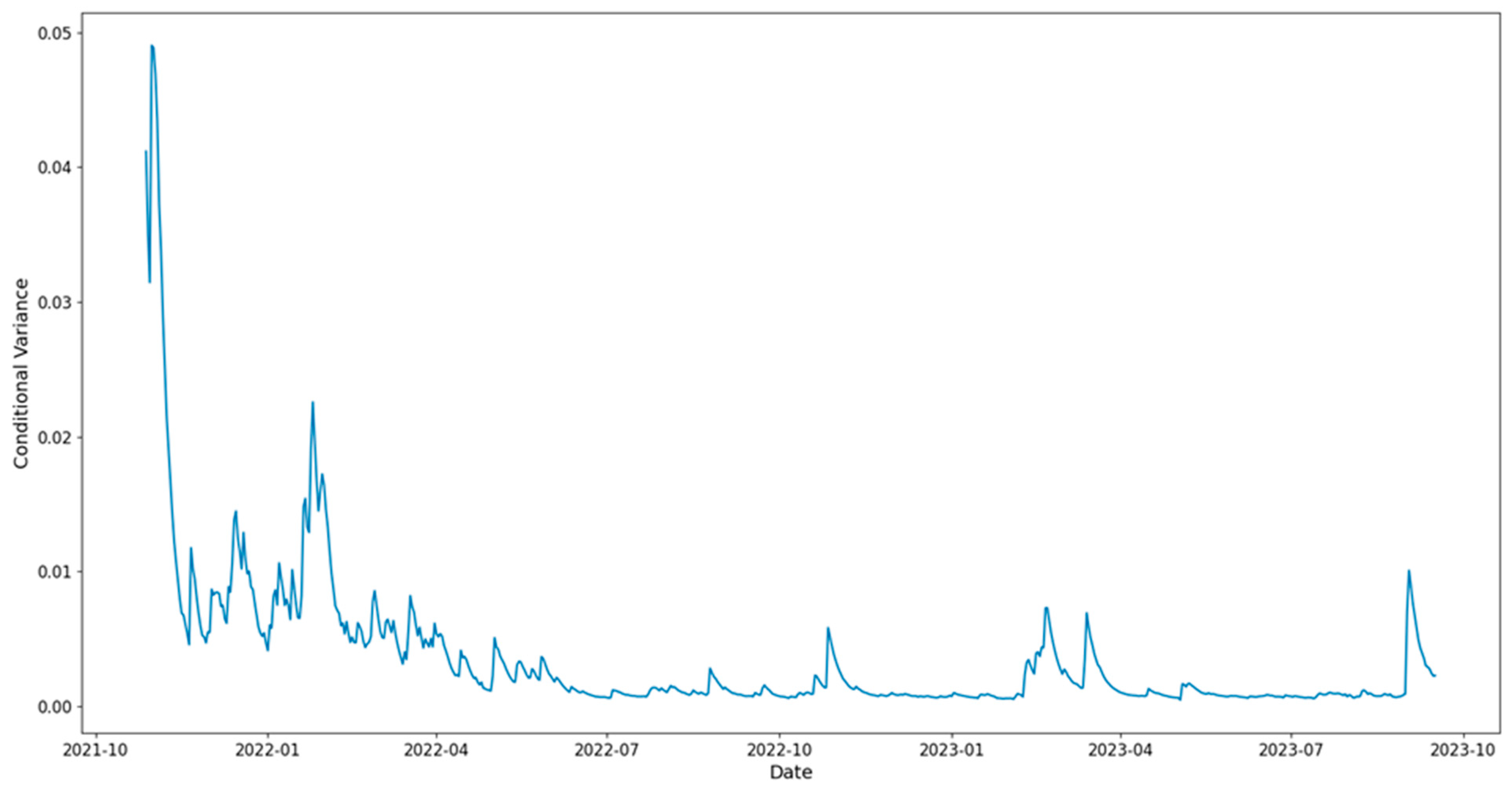
In Figure 3, we notice significant volatility fluctuations depicted by the conditional variance, particularly during the initial months of the time series. These early months exhibit exceptionally high values compared to the subsequent periods, indicating heightened volatility during this initial phase. However, there is a discernible pattern wherein the conditional variance experiences a sudden and significant drop following this initial period. Subsequently, the conditional variance stabilizes, remaining nearly constant with some sudden fluctuations for the remainder of the observed period. This pattern suggests a period of heightened uncertainty or volatility during the initial phase, possibly driven by specific market events or external factors, such as the sudden crash in December 2021, where approximately USD 300 billion reduced the crypto asset market in two days following an announcement by the United States Federal Reserve Bank (Azimli 2024). The subsequent decrease in conditional variance could indicate a period of relative stability or adjustment within the system, leading to reduced volatility levels. The sustained stability of conditional variance in the subsequent months implies a consistent level of volatility, highlighting the importance of understanding and monitoring the underlying factors driving these fluctuations over time. This uncertainty is evident for this period, where the total crypto asset market from a total market capitalization of approximately USD 3 trillion in early November 2021 fell to approximately USD 1.8 billion at the end of January 2022 and subsequently to about USD 900 billion by the end of June 2022 and remained at approximately these levels up to the late September 2023, according to data from Coingecko. A similar pattern is evident in the variable regarding the “Top 100 DeFi Coins” by Coingecko, which we used as a proxy for the comovement of similar assets, where in early November 2021, the variable had a value of approximately USD 160 billion, and at the end of January 2022, a value of approximately USD 105 billion and from the end of June 2022 up to the end of September 2023, the values range from USD 36 to 45 billion.

Possible explanations for the significant volatility fluctuations in the initial months could be spillover from the general crypto market, as in the fourth quarter of 2021 because of the effect of COVID-19 and the first and second quarter of 2022 because of the Russo-Ukrainian war, as documented by Poddar et al. (2023) in their research, which finds connectedness in the cryptocurrency returns for these periods.

5. Discussion

The results of the VAR model, Granger causality, and VECM analyses provide the policymakers, who in this context are the community that governs the protocols of the examined DAOs, with valuable insights into the dynamic interplay between OlympusDAO and KlimaDAO, facilitating informed decision making. The decision-making process might involve presenting a new proposal in the governance forums of the DAOs, which could entail altering the allocation of their treasury or adjusting parameters such as the rebasing frequency or token staking yield rates. The VAR model reveals the short-term dependencies and interactions between the variables of interest, such as the treasury balances and the token prices, and other relevant factors, such as the “Top 100 DeFi Coins by Market Capitalization” index.

Granger causality analysis identifies the direction and significance of causal relationships between the variables, aiding policymakers in understanding which DAO may influence the other and to what extent. The outcomes of the Granger causality tests, as depicted in the results section, elucidate compelling relationships within our study. The significant causal connection between the returns of OlympusDAO MC, the returns of KlimaDAO MC, and the returns of their treasuries suggests that these factors may hold predictive value for their future returns.

Additionally, the VECM model captures the long-term equilibrium relationships between OlympusDAO and KlimaDAO, helping policymakers anticipate how changes in one DAO’s treasury or token values may affect the other over time. By considering these results collectively, policymakers can devise strategies to better manage funds related to OlympusDAO and KlimaDAO and optimize their resource allocation.

Furthermore, after examining the KlimaDAO treasury, we observe that the returns of KCT may also affect the KlimaDAO conditional variance. For policymakers, identifying KCT as statistically significant in the conditional variance equation offers valuable insights into the determinants of volatility within the system under consideration. Understanding the factors driving volatility is crucial for designing effective policy interventions to promote stability and mitigate risks regarding managing a portfolio containing KlimaDAO tokens.

While this study provides valuable insights into the interaction between market capitalization and treasuries within specific DAO projects, namely OlympusDAO and KlimaDAO, several limitations warrant consideration. Firstly, the scope of the research is confined to these particular projects, potentially limiting the generalizability of findings to other DeFi contexts or similar DAO projects because of differences in their economic model, the underlying assets in their treasury, and the utility of the DAO-issued tokens. Secondly, while Granger causality tests offer insights into potential causal relationships, they do not establish causality definitively, making alternative interpretations possible. Moreover, the sample size of both the daily and monthly data may not fully represent the overall behavior of the treasury and the interaction between the two projects under examination, given that it spans approximately two years. Furthermore, the econometric models could also be extended to include more complexities inherent in market dynamics by including additional essential factors influencing the relationships studied, such as events regarding regulatory concerns or market conditions, trading volume from both decentralized and centralized exchanges, user interaction and sentiment analysis, staking rewards, and token supply dynamics. Finally, this study’s acknowledgment of regulatory uncertainties underscores the need for further investigation into the evolving regulatory landscape and its implications for tokenized assets within DAO treasuries. Addressing these limitations in future research endeavors will be crucial to advancing our understanding of decentralized finance dynamics and enhancing the applicability of findings to real-world contexts.

6. Conclusions

This study explored the interaction between market capitalization and treasuries in two popular DAO projects, OlympusDAO and KlimaDAO. Furthermore, we explored the effect of the returns of KlimaDAO treasury carbon tokens on KlimaDAO market capitalization returns’ conditional volatility.

The results could contribute to the predictive modeling toolkit, emphasizing the utility of the returns of OlympusDAO MC and shedding light on the distinct behaviors of OlympusDAO and KlimaDAO. The discoveries could offer investors valuable insights, aiding them in identifying additional variables like the DAO treasury and carbon token offsets to better understand the dynamics of the two DAOs and make more informed investment decisions. Policymakers, potentially the governing bodies of the DAOs, could adjust their treasury allocation strategies and the parameters of the DAO smart contracts to align with current market trends. Additionally, policymakers, which could be market regulators, may recognize the influence of carbon tokens on DAO market capitalization, providing further support for the efficacy of this new technology in tokenizing carbon offsets, which could lead to the expansion and organization of carbon offset markets on the blockchain. Researchers can now emphasize the significance of DAO treasuries and the impact of carbon offset tokens, thereby extending research into the importance of other DAO treasuries and potentially tokenized assets.

This study could be a headstart to support whether questionable tokenized assets could be considered to have value or some other form of financial impact. It also provides more evidence that if a token is backed by assets in a DAO treasury, these assets could influence the token’s value dynamics, enabling the potential managers of such assets to make better investment decisions. This study’s contribution lies in examining the intricate interplay between market capitalization and treasuries within prominent DAO projects, such as OlympusDAO and KlimaDAO, along with the potential influence of treasury-held carbon tokens on market capitalization returns. By elucidating these dynamics, the research augments the existing literature by providing insight into the behavioral patterns between DAOs and sheds light on tokenized asset valuation mechanisms.

One significant innovation of this research lies in its investigation of the influence of environmental factors and the necessity to comprehend the functioning of market dynamics that incorporate these variables. Furthermore, our study delves into sustainability concerns within the crypto asset ecosystem and explores the convergence of environmental preservation and blockchain technology, offering potential avenues for advancing eco-friendly advancements within the digital asset realm.

These findings enrich our understanding of decentralized finance dynamics, offering practical implications for investors, policymakers, and researchers. An implication is that the DAOs are related to the DeFi market cap index examined in this study. Another implication is that this study could be used as a benchmark to create an investment strategy in the future when including the examined variables of this study. Finally, this study underscores the significance of responsible investing, demonstrating its efficacy not only in advancing environmental and social welfare goals but also as a robust investment strategy, suggesting the potential for expanding the scope of sustainable investment assets or indices, which not only prioritize social welfare but also offer profitable returns for investors.

Furthermore, this research explored the importance of a DAO’s treasury and identified a potential link between the returns from the carbon offset tokens stored in the treasury, which may contribute to the market capitalization returns volatility of the DAO when employed as collateral for its token, even in the presence of regulatory uncertainties, providing a foundational framework for informed investment decisions and future research endeavors within the field. While prior studies have illuminated these projects’ organizational and innovative frameworks, this is the first study to undertake an econometric evaluation as a pioneering effort to offer such invaluable insight.

Future studies could focus on further evaluating the significance of the treasury in DeFi projects, emphasizing its role in assessing the overall value of a DeFi project. Finally, there is an opportunity for scholarly inquiry to extend into appraising the relevance of alternative tokenized assets within this framework.

References

- Ante, Lennart, Ingo Fiedler, Jan Marius Willruth, and Fred Steinmetz. 2023. A Systematic Literature Review of Empirical Research on Stablecoins. FinTech 2: 34–47. [Google Scholar] [CrossRef]
- Armisen, Albert, Clara-Eugènia de-Uribe-Gil, and Núria Arimany-Serrat. 2024. Navigating Carbon Offsetting: How User Expertise Influences Digital Platform Engagement. Sustainability 16: 2171. [Google Scholar] [CrossRef]
- Azimli, Asil. 2024. Time-Varying Spillovers in High-Order Moments among Cryptocurrencies. Financial Innovation 10: 96. [Google Scholar] [CrossRef]
- Babel, Matthias, Vincent Gramlich, Marc-Fabian Körner, Johannes Sedlmeir, Jens Strüker, and Till Zwede. 2022. Enabling End-to-End Digital Carbon Emission Tracing with Shielded NFTs. Energy Informatics 5: 27. [Google Scholar] [CrossRef]
- Baim, Owen. 2023. Curbing Climate Change: An Analysis of the Blockchain’s Impact on the Voluntary Carbon Market. Available online: https://doi.org/10.7302/7176 (accessed on 2 November 2023).
- Bhambhwani, Siddharth. 2023. Governing Decentralized Finance (DeFi). Available online: https://doi.org/10.2139/ssrn.4513325 (accessed on 8 November 2023).
- Bollerslev, Tim. 1986. Generalized Autoregressive Conditional Heteroskedasticity. Journal of Econometrics 31: 307–27. [Google Scholar] [CrossRef]
- Bordeleau, Erik, and Nathalie Casemajor. 2023. Cosmo-Financial Imaginaries: BeeDAO as Infrastructural Art Prototype for Planetary Regeneration. Available online: https://doi.org/10.31235/osf.io/hmx68 (accessed on 8 November 2023).
- Buterin, Vitalik. 2014. Ethereum: A Next-Generation Smart Contract and Decentralized Application Platform. Available online: https://blog.ethereum.org/2014/05/06/daos-dacs-das-and-more-an-incomplete-terminology-guide (accessed on 10 April 2024).
- ChatGPT. n.d. Available online: https://chat.openai.com (accessed on 9 April 2024).
- Chitra, Tarun, Kshitij Kulkarni, Guillermo Angeris, Alex Evans, and Victor Xu. 2022. DeFi Liquidity Management via Optimal Control: Ohm as a Case Study. Available online: https://people.eecs.berkeley.edu/~ksk/files/Ohm_Liquidity_Management.pdf (accessed on 9 September 2023).
- CoinGecko. n.d. Cryptocurrency Prices, Charts, and Crypto Market Cap. Available online: https://www.coingecko.com/ (accessed on 26 October 2023).
- DefiLlama. n.d. DefiLlama—DeFi Dashboard. Available online: https://defillama.com/ (accessed on 23 October 2023).
- Dobrajska, Magdalena. 2023. Klima DAO: An Intermediary in a Nascent Market. Journal of Organization Design 12: 285–87. [Google Scholar] [CrossRef]
- Engle, Robert F. 1982. Autoregressive Conditional Heteroscedasticity with Estimates of the Variance of United Kingdom Inflation. Econometrica 50: 987–1007. [Google Scholar] [CrossRef]
- Engle, Robert F., and Clive W. J. Granger. 1987. Co-Integration and Error Correction: Representation, Estimation, and Testing. Econometrica 55: 251–76. [Google Scholar] [CrossRef]
- Foss, Nicolai J., and Tianjiao Xu. 2023. Unveiling the Familiar in the Unconventional: The Case of Klima DAO. Journal of Organization Design 12: 289–91. [Google Scholar] [CrossRef]
- Freni, Pierluigi, Enrico Ferro, and Roberto Moncada. 2022. Tokenomics and Blockchain Tokens: A Design-Oriented Morphological Framework. Blockchain: Research and Applications 3: 100069. [Google Scholar] [CrossRef]
- Ghodoosi, Farshad. 2022. Crypto Litigation: An Empirical View. Available online: https://papers.ssrn.com/abstract=4288024 (accessed on 21 February 2024).
- Glosten, Lawrence R., Ravi Jagannathan, and David E. Runkle. 1993. On the Relation between the Expected Value and the Volatility of the Nominal Excess Return on Stocks. The Journal of Finance 48: 1779–801. [Google Scholar] [CrossRef]
- Grammarly: Free AI Writing Assistance. n.d. Available online: https://www.grammarly.com/ (accessed on 9 April 2024).
- Guo, Jinyan, Qevan Guo, Chenchen Mou, and Jingguo Zhang. 2024. A Mean Field Game Model of Staking Systemand A Reinforcement Learning Framework for Parameter Optimization. Available online: https://doi.org/10.21203/rs.3.rs-3872334/v1 (accessed on 12 April 2024).
- He, Vivianna Fang, and Phanish Puranam. 2023. Some Challenges for the ‘New DAOism’: A Comment on Klima DAO. Journal of Organization Design 12: 293–95. [Google Scholar] [CrossRef]
- Jirásek, Michal. 2023. Klima DAO: A Crypto Answer to Carbon Markets. Journal of Organization Design 12: 271–83. [Google Scholar] [CrossRef]
- Johansen, Søren. 1991. Estimation and Hypothesis Testing of Cointegration Vectors in Gaussian Vector Autoregressive Models. Econometrica 59: 1551–80. [Google Scholar] [CrossRef]
- KlimaDAO. 2022. The KLIMA Token’s Role in the Digital Carbon Market. Available online: https://www.klimadao.finance/blog/what-is-KLIMA-tokens-role-in-onchain-carbon-market (accessed on 8 August 2022).
- Maker Team. 2017. The Dai Stablecoin System. Available online: https://makerdao.com/whitepaper/DaiDec17WP.pdf (accessed on 15 April 2024).
- Metelski, Dominik, and Janusz Sobieraj. 2022. Decentralized Finance (DeFi) Projects: A Study of Key Performance Indicators in Terms of DeFi Protocols’ Valuations. International Journal of Financial Studies 10: 108. [Google Scholar] [CrossRef]
- Mislavsky, Robert. 2024. Behavioral Tokenomics: Consumer Perceptions of Cryptocurrency Token Design. Available online: https://doi.org/10.2139/ssrn.4686759 (accessed on 12 April 2024).
- Murray, Alex, Dennie Kim, and Jordan Combs. 2023. The Promise of a Decentralized Internet: What Is Web3 and How Can Firms Prepare? Business Horizons 66: 191–202. [Google Scholar] [CrossRef]
- Nelson, Daniel B. 1991. Conditional Heteroskedasticity in Asset Returns: A New Approach. Econometrica 59: 347–70. [Google Scholar] [CrossRef]
- Nowak, Eric. 2022. Voluntary Carbon Markets. Available online: https://papers.ssrn.com/abstract=4127136 (accessed on 8 November 2023).
- Oguntegbe, Kunle Francis, Nadia Di Paola, and Roberto Vona. 2023. Traversing the Uncommon Boulevard: Entrepreneurial Trajectory of Decentralised Autonomous Organisations (DAOs). Technology Analysis & Strategic Management, 1–17. [Google Scholar] [CrossRef]
- Olympus Docs. n.d. Treasury. Available online: https://docs.olympusdao.finance/main/overview/treasury/ (accessed on 10 November 2023).
- Poddar, Abhishek, Arun Kumar Misra, and Ajay Kumar Mishra. 2023. Return Connectedness and Volatility Dynamics of the Cryptocurrency Network. Finance Research Letters 58: 104334. [Google Scholar] [CrossRef]
- Poon, Ser-Huang, and Clive W. J. Granger. 2003. Forecasting Volatility in Financial Markets: A Review. Journal of Economic Literature 41: 478–539. [Google Scholar] [CrossRef]
- Pupyshev, Aleksei, Ilya Sapranidi, and Shamil Khalilov. 2022. Pathway: A Protocol for Algorithmic Pricing of a DAO Governance Token. arXiv arXiv:2202.06541. [Google Scholar] [CrossRef]
- Rossello, Romain. 2024. Blockholders and Strategic Voting in DAOs’ Governance. Available online: https://doi.org/10.2139/ssrn.4706759 (accessed on 22 February 2024).
- Schletz, Marco, Axel Constant, Angel Hsu, Simon Schillebeeckx, Roman Beck, and Martin Wainstein. 2023. Blockchain and Regenerative Finance: Charting a Path toward Regeneration. Frontiers in Blockchain 6: 1165133. [Google Scholar] [CrossRef]
- Shojaie, Ali, and Emily B. Fox. 2022. Granger Causality: A Review and Recent Advances. Annual Review of Statistics and Its Application 9: 289–319. [Google Scholar] [CrossRef] [PubMed]
- Sicilia, Miguel-Angel, Elena García-Barriocanal, Salvador Sánchez-Alonso, Marçal Mora-Cantallops, and Juan-José de Lucio. 2022. Understanding KlimaDAO Use and Value: Insights from an Empirical Analysis. In International Conference on Electronic Governance with Emerging Technologies. Cham: Springer, pp. 227–37. [Google Scholar]
- Sipthorpe, Adam, Sabine Brink, Tyler Van Leeuwen, and Iain Staffell. 2022. Blockchain Solutions for Carbon Markets Are Nearing Maturity. One Earth 5: 779–91. [Google Scholar] [CrossRef]
- Song, Ahyun, Euiseong Seo, and Heeyoul Kim. 2023. Analysis of Olympus DAO: A Popular DeFi Model. Paper presented at 2023 25th International Conference on Advanced Communication Technology (ICACT), Pyeongchang, Republic of Korea, February 19–22; pp. 262–66. [Google Scholar] [CrossRef]
- Sorensen, Derek. 2023. Tokenized Carbon Credits. Ledger 8: 76–91. [Google Scholar] [CrossRef]
- Spinoglio, Francesco. 2022. Redefining Banking Through Defi: A New Proposal for Free Banking Based on Blockchain Technology and DeFi 2.0 Model. Journal of New Finance 2: 1. [Google Scholar] [CrossRef]
- Verra. 2021. Verra Statement on Crypto Market Activities. Verra (Blog). Available online: https://verra.org/statement-on-crypto/ (accessed on 25 November 2021).
- Verra. 2022. Verra Addresses Crypto Instruments and Tokens. Verra (Blog). Available online: https://verra.org/verra-addresses-crypto-instruments-and-tokens/ (accessed on 25 May 2022).
- Verra. 2023. Verra Concludes Consultation on Third-Party Crypto Instruments and Tokens. Verra (Blog). Available online: https://verra.org/verra-concludes-consultation-on-third-party-crypto-instruments-and-tokens/ (accessed on 17 January 2023).
- Ziegler, Christian, and Isabell M. Welpe. 2022. A Taxonomy of Decentralized Autonomous Organizations. Available online: https://aisel.aisnet.org/icis2022/blockchain/blockchain/1 (accessed on 6 October 2023).
- Zotero. n.d. Your Personal Research Assistant. Available online: https://www.zotero.org/ (accessed on 9 April 2024).
Figure 1.
Box plots of the examined daily value variables.
Figure 2.
Box plots of the examined monthly value variables.
Figure 3.
GARCH results: conditional variance.