1. Introduction
Stress test scenarios for credit risk typically are stated in terms of economic factors but sometimes involve defaults of larger counterparties or obligors (see e.g., Section 10.3.3 of [
1]). Default of a large obligor not only has a direct impact on the profit and loss of a bank and potentially also on its capital basis. Due to mutual dependence of default events the default of one or more obligors can have a significant impact on the loss distribution of the remaining portfolio, too. Determination of credit portfolio loss distributions conditional on defaults, therefore, can be considered a special stress testing technique. Such analysis, in particular, can help to decide whether a large exposure to a certain obligor is just a risk concentration because of its size or, even worse, also significant part of a sector or industry risk concentration. Loss distributions conditional on default of one or more obligors therefore are promising means to identify vulnerabilities of banks.
Techniques for measuring the impact of macro-economic stress scenarios on credit portfolio losses are well-established (see e.g., [
2,
3]). In particular, it is common and efficient to analyse such stress scenarios by means of Monte Carlo simulation. In principle, it is easy to determine also the impact of the default of one or more obligors via a Monte Carlo simulation approach: just eliminate all simulation iterations from the sample in which the obligor(s) on whose default(s) conditioning is to be conducted have not defaulted. This is feasible in practice for one default but becomes impracticable for two or more defaults.
An obvious approach to try and work around this problem would be to deploy an unstressed (i.e., unconditional) model for the analysis but to feed it with parameters like probabilities of default (PDs) and loss-given-default (LGD) that have been stressed in a separate exercise before. This approach—which may be called the “stressed input parameters” approach—might fail, however, to fully capture the dependence structure of the model and its changes under stress such that misjudgement of the stress impact could be the consequence.
This paper seeks to assess how accurate the results calculated with the “stressed input parameters” approach are when compared to results from a fully-fledged conditional loss distribution approach. For that purpose we revisit the CreditRisk
credit portfolio risk model [
4] and derive a representation of the loss distribution conditional on the default of two fixed obligors that allows for the computation of the distribution without Monte Carlo simulation. Two numerical examples then suggest that results from the stressed input parameters approach may be seriously inaccurate but tend to be inaccurate in a conservative direction and to overestimate tail losses.
Tasche [
5] (Equation (3.31)) showed how the loss distribution conditional on one default can be calculated analytically in the CreditRisk
model with random loss severities. In this paper, the related formulas for the case of two defaults are provided. Formulas for the cases of three or more defaults can be readily derived in the same way as the formula for the case of two defaults is derived. As a consequence of the likely lack of practical relevance of cases of three or more defaults scenarios, we do not provide the results for these cases here. Moreover, the paper is focused on the theoretical derivation of the main result on the loss distribution conditional on two defaults and its interpretation. The question of practical numerical implementation is only considered to such an extent as needed for the numerical examples.
The plan of this paper is as follows:
As background and for introducing the notation,
Section 2 provides a description of the CreditRisk
model as presented in [
4] or [
6]. The CreditRisk
model described here is enhanced to allow for random loss severities. Schmock [
7] describes a further generalisation of the model to include connected groups of obligors.
In
Section 3, the results on the conditional loss distributions are presented and their application is discussed. To derive the results, we revisit the approach used in [
5] to develop analytical representations of the Value-at-Risk and Expected Shortfall contributions of single obligors in CreditRisk
.
In
Section 4, we present the technical particulars of the stressed input parameters approach and prove that the first moments of the resulting loss distributions are the same as the first moments of the proper loss distribution conditional on two defaults.
Section 5 provides two numerical examples to shed light on the question of how close the results from the stressed input parameters and conditional loss distribution approaches are in general.
The paper concludes with summarising comments in
Section 6.
2. An Analytical Credit Portfolio Model with Random Loss Severities
The modelling of the default events in the CreditRisk
credit portfolio risk framework may be described as a Poisson mixture model ([
8], Section 8.4). Basically, there is a two-step random mechanism which first generates potentially correlated default intensities for each of the obligors in the portfolio and then realises independent Poisson variables with these intensities. If the realisation of an obligor’s Poisson variable takes a value greater than or equal to 1, then the obligor defaults and credit loss may be the consequence. If the realisation is 0, then the obligor remains solvent and no loss is incurred.
The approach to the CreditRisk
loss distribution as described in [
4] or [
6] is driven by analytical considerations and—to some extent—hides the way in which the Poisson approximation is used to smooth the loss distribution. While preserving the notation of [
6], therefore, we review in this section the steps that lead to the formula for the generating function of the loss distribution in [
4,
6]. When doing so, we slightly generalize the methodology to the case of stochastic exposures—thus allowing for random loss severities—that are independent of the default events and the random factors expressing the dependence on sectors or industries. This generalization can be afforded at no extra cost as the result is again a generating function in the shape as presented in Equation (2.19) of [
6], the only difference being that the sector polynomials are composed another way.
Write
for the default indicator of obligor
A,
i.e.,
if
A does not default in the observation period and
if
A defaults. In [
4,
6], an approximation is derived for the distribution of the portfolio loss variable
with the
denoting deterministic potential losses. A careful inspection of the beginning of Section 5 of [
6] reveals that the main step in the approximation procedure is to replace the
-valued indicators
by integer-valued random variables
with the same expected values. These variables
are conditionally Poisson distributed given some economic factors
.
Here, we want to study the distribution of the more general loss variable
, where
denotes the random outstanding exposure of obligor
A. We assume that
takes on non-negative integer values and is independent of
. However, just replacing
by
as in the case of deterministic potential losses does not yield a nice generating function—“nice” in the sense that the CreditRisk
algorithms for extracting the loss distribution can be applied. We instead consider the approximate loss variable
where
are independent copies of
. Thus, we approximate the terms
by conditionally compound Poisson sums. For the sake of brevity, we write
for the loss suffered due to obligor
A. In order to make all these approximations work, we make the following formal assumption.
Assumption 1. The distribution of the “loss” variable
X as defined by Equation (
1a) is specified by the following three properties:
- (i)
The approximate default indicators are conditionally independent given a vector of “economic” factors . The conditional distribution of given is Poisson with intensity where denotes the “probability of default” (PD) of obligor A and are “factor loadings” such that for each obligor A.
- (ii)
The idiosyncratic factor is a constant and equals 1. The factors are independent and Gamma-distributed with unit expectations and parameters for . We call a positive random variable Y Gamma-distributed if it has a density , for some parameters , . The function Γ denotes the familiar Gamma function generalising the factorial. is implied by the assumption that has unit expectation.
- (iii)
The random variables
are independent copies of a non-negative integer-valued random variable
and, additionally, are also independent of the
and
. The distribution of
is given by its generating function
A careful inspection of the arguments presented to derive Equation (2.19) of [
6] now yields the following result on the generating function of the distribution of the loss variable
X.
Theorem 2. Under Assumption 1, define for the sector polynomial bywhere the sector default intensities are given byThen, the generating function , , of the loss variable X can be represented aswhere the constants are defined as . Remark 1. - (i)
The case of deterministic severities can be regained from Theorem 2 by choosing the exposures constant, e.g. . Then the generating functions of the exposures are just monomials, namely .
- (ii)
Representation Equation (
2c) of the generating function of the portfolio loss distribution implies that the portfolio loss distribution can be interpreted as the distribution of a sum of
independent sector loss distributions that correspond to the economic factors
.
The term
is the generating function of a random variable with a compound Poisson distribution that can be realised as
where
are independent,
is Poisson distributed with intensity
, and
are i.i.d. with generating function
. See, e.g., [
9] for background information on compound distributions and generating functions.
The terms , , are the generating functions of random variables with compound negative binomial distributions that can be realised as where are independent, is negative binomially distributed with failure probability and size parameter , and are i.i.d. with generating function . We call a random variable Y with values in the non-negative integers negative binomially distributed with size parameter and failure probability if for . If the size parameter a of a negative binomial distribution is a positive integer then the distribution can be interpreted as the distribution of the number of failures in a series of independent identical experiments before the a-th success is observed.
With this representation of the portfolio loss distribution as the convolution of compound Poisson and negative binomial distributions, the sector polynomials can be interpreted as the generating functions of typical loss severities in the respective sectors.
By means of Theorem 2, the loss distribution of the generalized model Equation (
1a) can be calculated in principle with the same algorithms as in the case of the original CreditRisk
model. Once the probabilities
,
x non-negative integer, are known, it is an easy task to calculate the loss quantiles
as defined by
or related risk measures like Value-at-Risk or Expected Shortfall.
When working with Theorem 2, one has to decide whether random exposures shall be taken into account, and in case of a decision in favour of doing so, how the exposure distributions are to be modeled. [
5] (in Example 1) and [
7] present some possible choices of discrete exposure distributions. [
10] discusses an approximate but similar approach to random severities with continuous distributions.
Parametrisation of the factor model as described in Theorem 2 is non-trivial because the assumption of independent economic factors is unrealistic in practice. [
11] discusses how to derive appropriate factor loadings from default observations and their correlations. [
12] suggests introducing a further factor to model dependence of the economic factors without violating the assumptions of the framework. Their approach is generalised in [
13]. Other authors (e.g. [
14]) propose extensions of the CreditRisk
model that allow for realistic modelling of the dependencies between the economic factors but renounce the analytic tractability of the original model. [
15] discusses the impact on the loss distribution of choosing different factor dependence structures in extended versions of the CreditRisk
framework.
3. Loss Distributions Conditional on Defaults
The purpose of this section is to provide formulas for the portfolio loss distribution conditional on defaults that can be represented in similar terms as the unconditional loss distribution and hence be evaluated with the familiar CreditRisk
algorithms. The following theorem—a modification of Lemma 1 of [
5]—yields the foundation of the results. Denote by
the indicator variable of the event
E,
i.e.,
if
and
if
.
Theorem 3. Under Assumption 1, let be obligors such that for . It then holds thatfor any non-negative integer x, where the random variables on the right-hand side of Equation (4) are independent of the loss variable X and the default intensities . Proof of Theorem 3. We provide the proof only for the case
as the proof for general
r is not much different, but the notation would be more cumbersome. Hence, assume that two obligors
have been selected. The independence and conditional independence of Assumption 1 then imply
as stated in Equation (4). ☐
As the variable
approximates obligor
A’s default indicator the conditional expectation
can be interpreted as an approximation of the conditional probability of obligor
A’s default given that the portfolio loss
X assumes the value
x. In Corollary 1, [
5] observed the following result for
. It can be readily derived from Theorem 3.
Notation. For any positive integers define the n-dimensional i-th unit vector bywhere the dimension is known from the context we write for short. Corollary 4 (Probability of default conditional on portfolio loss).
Adopt the setting and the notation of Assumption 1 and Theorem 2. Write for in order to express the dependence of the portfolio loss distribution upon the exponents in (2c). Of course, the distribution also depends on , , and . However, these input parameters here are considered constant. Assume that x is an integer such that . Then, in the CreditRisk framework, the conditional probability of obligor A’s default given that the portfolio loss X assumes the value x can be approximated bywhere stands for a random variable that has the same distribution as but is independent of X. Intuitively, one might think that
would be a better approximation of the conditional probability of default of obligor
A than
. However, there is no such relatively simple representation of
as Equation (5) is for
. Moreover, by the assumption on the parametrisation of the conditional Poisson distribution of
we have
Hence, the bias of
with respect to
is likely to be greater than the bias of
.
The probabilities in the numerator of the right-hand side of Equation (5) must be calculated by convolution if the loss severities
are non-deterministic. In any case, Corollary 4 can be used for constructing the portfolio loss distribution conditional on the default of an obligor. Observe that, by the very definition of conditional probabilities, it follows that
Since, by Corollary 4, an approximation for
is provided, the term-wise comparison of Equations (5) and (7) yields
Note that, according to Equation (8), the conditional distribution of the portfolio loss X given that A defaults may be computed as a weighted mean of stressed portfolio loss distributions. The stresses are expressed by the exponents in the generating functions of , . In actuarial terms, incrementing the size parameter of a negative binomial claim number distribution (cf. Remark 1) means to give the claim number distribution a heavier tail. Hence, this way the number of claims (sector-related defaults in CreditRisk terms) tends to be larger after the stress was applied. No change due to stress, however, occurs to the sector loss severity distributions as characterised by the sector polynomials . This is no surprise, as the loss severities in the setting of this paper are assumed to be independent of the economic factors that drive the sector default frequencies.
Remark 2. - (i)
By Equation (8), stressed portfolio loss distributions can be evaluated, conditional on the scenarios that single obligors have defaulted. If, for instance, the portfolio Value-at-Risk changes dramatically when obligor A’s default is assumed, then one may find that the portfolio depends too strongly upon A’s condition.
- (ii)
Equation (8) reflects a write-off or special provision due to obligor A’s default. This is a consequence of the fact that, on the right-hand side of the equation, loss distributions of the shape appear, thus implying that losses X are added to a loss socket caused by obligor A’s first default. However, usually in banks occurred losses are not taken into account for the determination of risk metrics (like quantiles as defined by Equation (3)) but are deducted from the banks available capital buffer. In that sense, Equation (8) does not appropriately reflect banks’ practice.
- (iii)
To deal with the issue observed in (ii), note that Theorem 2 and Corollary 4 also can be applied to the case . In particular, dependencies within the portfolio are then still adequately reflected by obligor A’s conditional default intensity . While in Theorem 2 effectively eliminates any impact of obligor A on the unconditional portfolio loss distribution, Equation (8) clearly demonstrates the impact of the dependence between A and the rest of the portfolio on the conditional portfolio loss distribution.
While Theorem 3 can be used to study the portfolio loss distributions conditional on any number of defaults, we confine ourselves in the following corollary and its consequences to considering only the case of two defaults as we already did in the proof of Theorem 3. The formulas for conditioning on three or more defaults can be derived in the same way as the formula for the case of two defaults. The cases of three or more defaults, however, are notationally and computationally much more inconvenient, presumably much less relevant for practice, and do not add much more theoretical insight compared to the case of two defaults.
Corollary 5 (Joint probability of default conditional on portfolio loss).
Adopt the setting and the notation of Corollary 4. Let denote two obligors who have been selected in advance. Assume that x is an integer such that . Then, in the CreditRisk framework, the conditional joint probability of obligor ’s and obligor ’s default given that the portfolio loss X assumes the value x may be approximated bywhere for and stands for a random variable that has the same distribution as but is independent of X. While Equation (9) in general looks like a straight-forward extension of Equation (5), there is a subtle difference in the terms involving which reflect double stress in the same sector. This double stress is enforced by the additional factors .
Proof of Corollary 5. We derive Equation (9) by comparing the coefficients of two power series. The first one is
, the second one is an expression that is equivalent to
but involves generating functions similar to Equation (
2c).
Recall that we denote the generating function of
by
. By means of Theorem 3 and the independence of the random exposures, we can compute
Recall the definitions of the intensities
, the sector default intensities
and the sector polynomials
from Theorem 2. By making use of the fact that the economic factors
are Gamma-distributed with parameters
,
, and that
, we obtain for
(
cf. the proof of (3.25c) in [
5])
Denote by
the generating function of
X according to Equation (
2c) as a function of the exponents
on the right-hand side of the equation as has been explained in Corollary 4. Observe then that
Note that is the generating function of the sequence (i.e., of the distribution of ). Combining this observation with Equations (10a), (10b), and (12) implies Equation (9) by power series comparison. ☐
As Corollary 4 can be used for constructing the portfolio loss distribution conditional on the default of one obligor, Corollary 5 can be used for the portfolio loss distribution conditional on the joint default of two obligors. Again by the definition of conditional probabilities, it follows that
Since by Corollary 5 an approximation for
is provided, the term-wise comparison of Equations (9) and (13) yields
Making use of the well-known result (see Section 2.3 of [
6])
Equation (
14a) can be slightly simplified to
Comments similar to the comments on Equation (8) also apply to Equation (
14c). The conditional distribution
of the portfolio loss
X given that obligors
and
default can be computed as a weighted mean of stressed or double-stressed portfolio loss distributions. The stresses, however, are not only expressed by the exponents
and
in the generating functions of
and
,
, but also by the factors
appearing on the right-hand side of (
14c). Obviously, as a consequence of the
terms on the right-hand side of Equation (
14c) instead of the only
terms of the right-hand side of Equation (8), it is much more expensive to calculate the loss distributions conditional on two defaults than to calculate the loss distributions conditional on simple defaults.
Observe that Remark 2 also applies to Equation (
14c). Hence it makes sense to do the calculations for Equation (
14c) with loss severities
and
to reflect the risk management attitude not to take account of occurred losses for the determination of living portfolio risk metrics.
4. The “Stressed Probabilities of Default” Approach
Under the CreditRisk
framework, Equation (
14c) provides the algorithm needed for the calculation of the portfolio loss distribution conditional on the default of two obligors. However, if
N denotes the number of economic factors in the model, formula (
14c) requires the computation of
slightly different loss distributions which could be tedious if
N is large. In this section, therefore, we look at the “cheaper” alternative approach where the loss distribution is calculated only once according to Theorem 2 and all parameters but the unconditional probabilities of default
remain unchanged. Such stress testing procedures based on stressed input parameters are common practice in the banking industry [
16]. In the “stressed probabilities of default” approach the
are replaced by probabilities of default conditional on the default of the two obligors. The approach is based on the following three-events version of Equation (
14b).
Proposition 6. Under Assumption 1, let be obligors such that for . Then it holds that Proof of Proposition 6. The assumption on the Poisson distribution of the
conditional on the vector of economic factors
implies
with
defined as in Assumption 1 (i). By the conditional independence of
, therefore, it follows that
Recall that by assumption we have
for all
and
for all obligors
A. This implies
From the assumption that
is Gamma-distributed with parameter vector
, it follows that
and
. This implies the assertion. ☐
Since in the CreditRisk
framework the default indicator for an obligor
A is approximated by the conditional Poisson variable
, the joint probability of default
of three obligors is approximated by
Hence, Proposition 6 and Equation (
14b) provide us with a simple approximation formula for one obligor’s probability of default conditional on two other obligors’ joint default:
for any three different obligors
B,
and
. Thanks to Proposition 6 and Equation (
15), we can describe in precise technical terms the two above mentioned approaches to the calculation of the loss distribution conditional on two defaults.
Definition 7. Under Assumption 1, assume that there are two obligors
and
with exposures
. Call this setting the two defaults scenario. In addition, define the following two distributions:
- (i)
The portfolio loss distribution defined by the right-hand-side of Equation (
14c) is called the “two defaults scenario” loss distribution.
- (ii)
Replace in (i) of Theorem 2 the probabilities of default
by the conditional probabilities of default
as given by Equation (
15) and keep all other parameters in the theorem unchanged. The resulting portfolio loss distribution is called “stressed probabilities of default” loss distribution.
Intuitively, it is clear that the expected value
of the portfolio loss
X should be the same under both loss distributions from Definition 7. However, since the right-hand-sides of both Equation (
14c) and Equation (
15) are only approximations to the conditional probabilities on the left-hand-sides of the equations, the fact that the two expected values are equal must be formally proven.
Proposition 8. Under the ‘two defaults scenario’, denote by the distribution of Definition 7 (i) and by the distribution of Definition 7 (ii). Then it holds that .
Proof of Proposition 8. For the sake of a clear notation, we denote all obligors but
and
with the letter
B. Under the independence assumptions of Assumption 1, by construction of
Equation (
1a) implies that
For
, we obtain from Equation (
14c) that
The distributions of
X referred to in the expected values on the right-hand-side of Equation (17) are specified by the generating function Equation (
2c). As explained in Remark 1 (ii), for instance, the distribution of
X under
is given by the convolution of a compound Poisson distribution with expected value
and
N compound negative binomial distributions with expected values
Substituting all these expected values into Equation (17) and taking into account that
for all
B gives
Some algebra shows that the sum of the terms after the last “=” sign divided by the factor
is equal to the right-hand-side of Equation (16). ☐
Why are the two defaults scenario loss distribution and the stressed probabilities of default loss distribution of Definition 7 different despite the first order equality of the two demonstrated in Proposition 8? They differ because does not account for correct conditional joint probabilities of default for two or more obligors. Nonetheless, it is not clear how much the two loss distribution can differ, given that their first moments are equal. In the next section, we will consider two simple numerical examples to compare the two loss distributions and assess how different they may be.
Another question refers to the nature of the input parameters
in Theorem 2,
i.e., the unconditional PDs of the obligors in the portfolio. In principle, these PDs should be “through-the-cycle” (TTC) PDs in the CreditRisk
framework. See [
17] for a formal definition of TTC PDs and a discussion of TTC v. PIT (point-in-time) PDs. Does is then make sense to use conditional PDs as input parameters to the model as in the stressed PDs approach? Actually, this question misses the point. For the stressed PDs approach only is meant to be a technical workaround for more demanding approaches like Monte Carlo simulation and the calculation of the proper loss distribution conditional on two defaults (the “two defaults scenario” distribution).
5. Numerical Examples
The first example we consider is a homogeneous portfolio with a one-factor dependence structure. For the factor, we choose a standard deviation of 0.8 which according to [
18] is in the centre of the range of observable default rate volatilities. Since the factor is assumed to be Gamma-distributed with mean 1, a standard deviation of 0.8 implies that the factor is Gamma-distributed with parameters
.
Example 1. We assume the setting of Assumption 1 with the following specifics:
There are n obligors all with PD . There is one economic factor S such that the conditional Poisson distribution of the default indicator is given by the intensity for all .
Two further obligors and with the same characteristics as the other obligors are known to have defaulted.
The factor S is Gamma-distributed with parameters .
The exposure to each of the obligors but the defaulters is 1. Hence, we have for the generating functions of the exposures for all i. The exposures to the two defaulters and are 0.
Having all exposures equal to 1 means that in this case the portfolio “loss” distribution is actually the distribution of the number of defaults in the portfolio,
i.e., we have
By Remark 1 (ii), it follows that in the CreditRisk
framework the unconditional distribution of
X is negative binomial and as such given by
Equation (
14c) implies that the distribution of
X conditional on the default of
and
is approximated by
Again by Remark 1 (ii), it follows that the “stressed probabilities of default” distribution
of
X in the sense of Definition 7 is given by
and
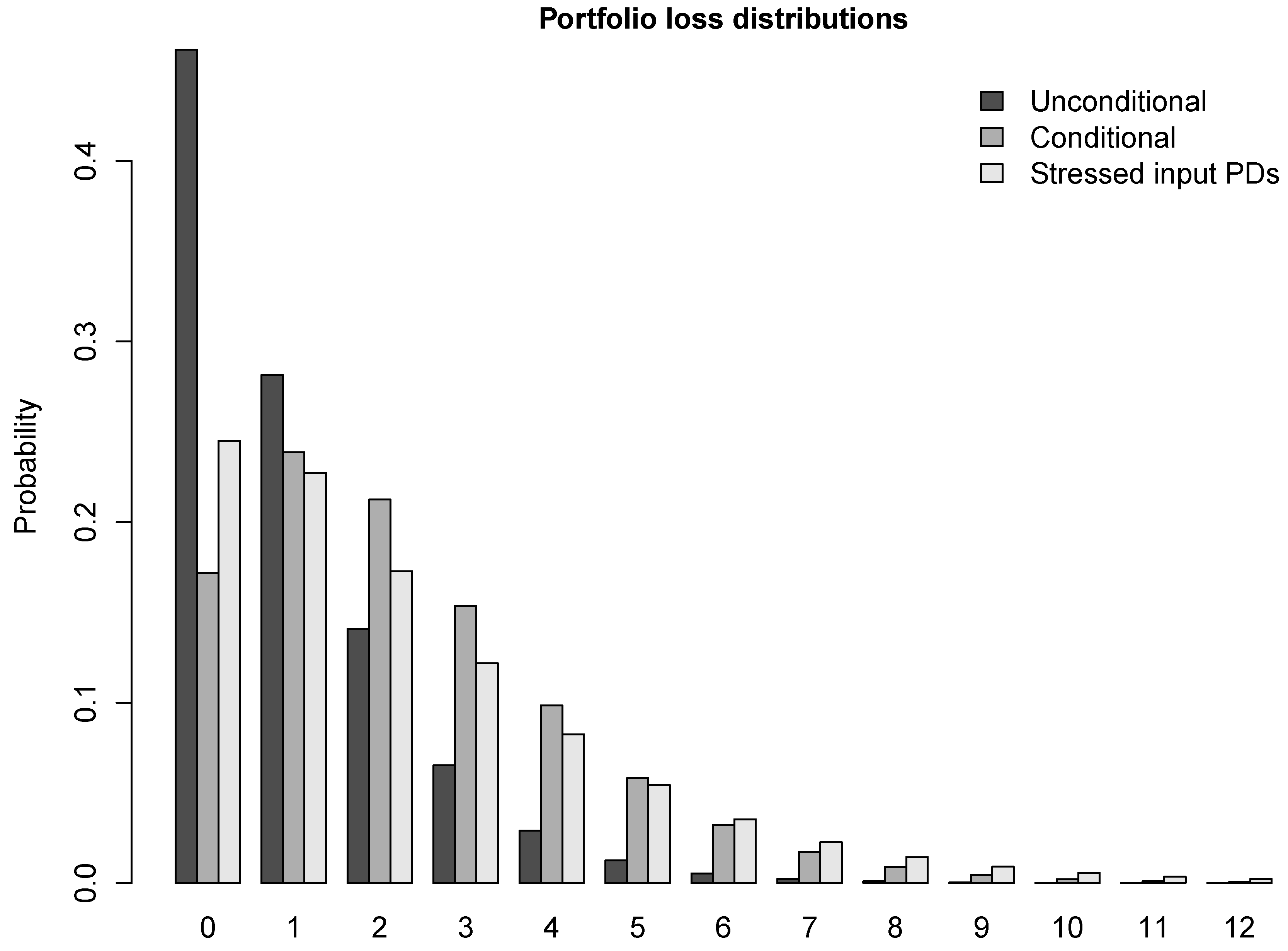
Figure 1 shows the three distributions from Example 1 for the case
. It is no surprise that, compared to the unconditional distribution, the masses of the other two distributions are significantly shifted to the right. But the “stressed input PDs” distribution seems to have heavier tails than the “two defaults scenario” distribution.
Figure 1.
Unconditional, conditional on two defaults and “stressed input PDs” distributions of the number of defaults in portfolio of 100 obligors. All obligors have unconditional PD 1%. The model is one-factor CreditRisk with factor standard deviation 0.8.
Figure 1.
Unconditional, conditional on two defaults and “stressed input PDs” distributions of the number of defaults in portfolio of 100 obligors. All obligors have unconditional PD 1%. The model is one-factor CreditRisk with factor standard deviation 0.8.
Table 1 affirms this observation. The results from the table suggest that the difference between the “two defaults scenario” and “stressed input PDs” distributions increases with growing portfolio size. The “stressed input PDs” distribution becomes markedly more widespread and heavier-tailed than the “two defaults scenario” distribution. A possible explanation could be that the “two defaults scenario” more appropriately takes account of diversification effects in the higher order joint probabilities of default that strongly impact the tail of the distribution because “two defaults” is constructed as a proper conditional distribution.
With the following example, we study a more heterogenous portfolio, with a range of different PDs, different exposures and dependence created by two economic factors. We choose standard deviations of 0.4 and 1.2 respectively for the two factors. According to [
18], this choice reflects the lower and upper bounds of the range of observable default rate volatilities.
Table 1.
Characteristics of unconditional, conditional on two defaults and “stressed input probabilities of default (PDs)” distributions of numbers of defaults in portfolios of , and obligors. All obligors have unconditional PD 1%. The model is one-factor CreditRisk with factor standard deviation 0.8.
| | Unconditional | “Two Defaults Scenario” | “Stressed Input PDs” |
|---|
| | | |
| Probability of no default | 0.9076 | 0.8017 | 0.8083 |
| Mean | 0.1000 | 0.2280 | 0.2280 |
| Standard deviation | 0.3262 | 0.4925 | 0.5111 |
| 99%-quantile | 1 | 2 | 2 |
| | | |
| Probability of no default | 0.4616 | 0.1716 | 0.2451 |
| Mean | 1.0000 | 2.2800 | 2.2800 |
| Standard deviation | 1.2806 | 1.9337 | 2.3679 |
| 99%-quantile | 5 | 8 | 10 |
| | | |
| Probability of no default | 0.0438 | 0.0008 | 0.0137 |
| Mean | 10.0000 | 22.8000 | 22.8000 |
| Standard deviation | 8.6023 | 12.9892 | 18.8546 |
| 99%-quantile | 39 | 63 | 87 |
Example 2. We assume the setting of Assumption 1, this time with the following specifics:
There are 60 obligors all with PD , 30 obligors all with PD and 10 obligors all with PD . There are two economic factors and such that the conditional Poisson distribution of the default indicator is given by the intensity with for all .
Two further obligors and are known to have defaulted. We assume they had PDs , and that their default intensities were given by . We assume . Results are calculated for two different values of , namely and .
The factor is Gamma-distributed with parameters , is Gamma-distributed with parameters .
Due to the heterogeneity of the portfolio in Example 2, it is not possible to represent the loss distribution of the loss variable
X in closed form. In order to calculate the unconditional, conditional on the two defaults and “stressed probabilities of default” distributions of
X as in Example 1; therefore, we take recourse to numerically inverting the respective characteristic functions by Fast Fourier Transform (FFT). Alternatively, we could have made use of refined versions of the Panjer algorithm as described in [
19] or Section 5.5 of [
20]. In all three cases, the shape of the characteristic function of the distribution is given by (
2c) with
,
. The algorithm we apply for the calculations is described in Section 4.7 of [
9]. The moderate size of the portfolio and the relatively small total exposure of the portfolio allow us to choose the total exposure plus 1 as the truncation point for the discrete Fourier transform. Indeed, the probabilities of the high losses close to the total exposure are so small that there is no need for any refinements of the algorithm to control the aliasing error (Section 2.2 of [
21]).
Table 2 shows the results of the calculations for Example 2. Results are reported for two different scenarios of dependence between the defaults and the rest of the portfolio:
“Weak dependence of defaults and portfolio” scenario. By construction, the obligors in the portfolio depend stronger on the economic factor (weight 0.75) than on the factor (weight 0.25). In the “weak dependence” scenario, the defaulters and depend weakly on (weight 0.25) and stronger on (weight 0.75).
“Strong dependence of defaults and portfolio” scenario. Here, the defaulters have the same dependence on the economic factors as the obligors in the portfolio.
In both dependence scenarios, the impact of conditioning on defaults on the tails of the loss distributions is strong, but it is much stronger in the case of strong dependence. In the weak dependence scenario, the shapes of the conditional “two defaults scenario” loss distribution and the “stressed input PDs” distribution seem to be almost equal. In contrast, in the strong dependence scenario, the tail of the “stressed input PDs” distribution appears to be much heavier than the tail of the “two defaults scenario” distribution. Note that, as stated in Proposition 8, in both
Table 1 and
Table 2, the means of the “two defaults scenario” and the “stressed input PDs” distributions always are equal.
Table 2.
Characteristics of unconditional, conditional on two defaults and “stressed input PDs” loss distributions of the portfolio described in Example 2. The model is two-factors CreditRisk.
Table 2.
Characteristics of unconditional, conditional on two defaults and “stressed input PDs” loss distributions of the portfolio described in Example 2. The model is two-factors CreditRisk.
| | Weak Dependence of Defaults and Portfolio |
|---|
| | Unconditional | “Two defaults scenario” | “Stressed input PDs” |
| Probability of no default | 0.2986 | 0.1769 | 0.1731 |
| Mean | 4.0000 | 6.7173 | 6.7173 |
| Standard deviation | 6.4900 | 9.0172 | 9.2574 |
| 99%-quantile | 30 | 41 | 43 |
| | Strong Dependence of Defaults and Portfolio |
| | Unconditional | “Two defaults scenario” | “Stressed input PDs” |
| Probability of no default | 0.2986 | 0.0545 | 0.0801 |
| Mean | 4.0000 | 11.4514 | 11.4514 |
| Standard deviation | 6.4900 | 11.5349 | 13.8041 |
| 99%-quantile | 30 | 52 | 64 |


