Article

Analysis of Dynamic Characteristic for Solar Arrays in Series and Global Maximum Power Point Tracking Based on Optimal Initial Value Incremental Conductance Strategy under Partially Shaded Conditions

1
College of Electrical Engineering and Automation, Tianjin University, Tianjin 300072, China
2
School of Electrical Engineering, Tianjin University of Technology, Tianjin 300384, China
3
College of Mechanical and Electrical Engineering, Northeast Forestry University, Harbin 150040, China
*
Author to whom correspondence should be addressed.
Energies 2017, 10(1), 120; https://doi.org/10.3390/en10010120
Submission received: 21 November 2016 / Revised: 31 December 2016 / Accepted: 12 January 2017 / Published: 19 January 2017

Abstract

:
Partial shading (PS) is an unavoidable condition which significantly reduces the efficiency and stability of a photovoltaic (PV) system. With PS, the system usually exhibits multiple-peak output power characteristics, but single-peak is also possible under special PS conditions. In fact it is shown that the partial shading condition (PSC) is the necessary but not sufficient condition for multiple-peak. Based on circuit analysis, this paper shows that the number of peak points can be determined by short-circuit currents and maximum-power point currents of all the arrays in series. Then the principle is established based on which the number of the peak points is to be determined. Furthermore, based on the dynamic characteristic of solar array, this paper establishes the rule for determination of the relative position of the global maximum power point (GMPP). In order to track the GMPP within an appropriate period, a reliable technique and the corresponding computer algorithm are developed for GMPP tracking (GMPPT) control. It exploits a definable nonlinear relation has been found between variable environmental parameters and the output current of solar arrays at every maximum power point, obtained based on the dynamic performance corresponding to PSC. Finally, the proposed method is validated with MATLAB®/Simulink® simulations and actual experiments. It is shown that the GMPPT of a PV generation system is indeed realized efficiently in a realistic environment with partial shading conditions.

1. Introduction

The renewable energy sources have been increasingly used to counter the problems with the conventional energy sources, such as the greenhouse effect, prices etc. Among those energy sources, the photovoltaic (PV) generation has great potential in terms of fuel cost (zero), scalability in power, simplicity in operation, and the maintenance required [1]. On the other hand, PV generation systems have low energy conversion efficiency because the solar cell exhibits nonlinear current versus voltage (I-V) and power versus voltage (P-V) characteristics. These nonlinear characteristics are functions of weather conditions such as solar insolation and cell temperature. PV systems often comprise many PV modules connected in series to achieve the required output voltage and power. When some of the modules receive lower solar irradiance due to occlusion of the sun by objects such as clouds, trees and buildings, a condition known as partially shaded condition (PSC), the output of the PV system is affected [2]. Usually when PSC occurs the system has multiple-peak output power characteristics. Only one of these peak powers has the highest power, which is called global maximum power point (GMPP), and other peak powers are the local maximum power point (LMPP). According to statistic studies the power loss can vary from 10% to 70% due to PS [3,4]. Moreover, under some special weak PS conditions, a PV system may have just one peak point. Therefore, the PSC is a necessary but not sufficient condition for multiple-peak. Finding the sufficient and necessary condition of multiple-peak is of course beneficial for analyzing the dynamic characteristic of solar arrays in series. In this paper, the circuit analysis method is used to determine the working principle of the photovoltaic array in series under PSC, and to explore the reasons for the phenomenon of multiple peak output power characteristics. Meanwhile, the sufficient and necessary condition of multiple-peak and the calculation method of the number of multiple peaks are presented in this paper.
To achieve the MPP, the maximum power point tracker (MPPT) is implemented as a controller to adjust the duty cycle of the power electronic part, which is an interface between the PV system and load [5,6]. Many MPPT methods have been developed and implemented, including the perturbation and observation (P&O) algorithm [7,8,9,10,11,12], which is known as the hill climbing (HC) method, the incremental conductance (INC) algorithms [11,13,14,15,16,17], the neural network (NN) method [18], and the fuzzy logic method [19,20]. These methods execute MPPT based on the fact that the slope of the P-V characteristic is equal to zero at MPP. Most of this type of control methods, like INC and P&O, could produce problems including a large delay, the inaccuracy of the detection circuits and sensors, and the power oscillation under low irradiation conditions [21,22]. But, these methods are still used extensively because of theirs high tracking accuracy at the steady state, flexibility to adapt to rapidly changing atmospheric conditions, and simplicity in application. Meanwhile, these drawbacks can be reduced by controlling the step size that is added or subtracted to the duty cycle.
It is worth noting that the aforementioned traditional MPPTs are not able to identify the GMPPT form the LMPPs when the PV characteristic curve consists of more than one peak [23]. Many algorithms were proposed to find the GMPP under shading condition with the aim to avoid the local maxima of the power while tracking the global maxima [24,25,26,27], which including the particle swarm optimization (PSO) methods [28], differential evolutionary and particle swarm optimization (DEPSO) methods [29], artificial intelligence techniques [30], neural network methods [26], scanning methods [27], equilibration algorithm [31]. These methods execute GMPPT by two ways: scanning method—swings the converter’s duty cycle from zero to one to determine the maximum power delivering capacity of the panel at a given operating condition and controls the power conditioning unit to extract the same from the PV panel; search algorithm—searching the global extreme of a function which describes the PV power and voltage or power and current relationship in an interval. The scanning program can find the GMPP at any condition, but it has a significant power loss because the program will frequently restart when the environmental condition changes. The search algorithms have the same issue during the computation of the open-circuit voltage and the short-circuit current [32]. From the perspective of maximizing the energy production of the PV array itself during its lifetime, the objective of the maximization of the energy production of a PV array during its lifetime is not necessarily in complete agreement with the objective of the maximization of its power production in any operating condition. It may be preferable to give up a part of the available energy today if it is possible to gain greater energy tomorrow. Based on the thought, some new methods have been proposed [33,34,35].
The problem of local minimum is caused by the fact that the existing MPPT methods tend to converge to the first peak closest to the algorithms’ operation initial value (OIV). In order to achieve the GMPP, the OIV of the algorithms should be placed within the GMPP zone or at least nearby. But this requires the knowledge of the GMPP zone or an algorithm that could determine I p m a x in PS conditions. Therefore, it is the first task of this paper to present the proposed control strategy for the purpose of finding the GMPP zone rapidly in real-time.
The GMPP zone and I p m a x of the solar arrays in series depend on the every cell’s environmental conditions, including the temperature of the solar cell and the irradiance of sunlight [26,36,37,38,39]. Thus, it is necessary to adopt the environmental parameters directly as the input variables to compute the I p m a x and GMPP zone under PSC. In practice, there are many MPPT control methods which adopt irradiance and temperature as the parameters to calculate the control reference signal [21,37,38,39]. However, all of them must use the irradiance and temperature sensors, which maybe problematic because, on the one hand, the irradiance cannot be accurate measured under PSC; on the other hand, the measurement error of the sensors brings significant uncertainty even under normal environmental conditions. Moreover, the use of the sensors increases the cost of the system. To avoid such difficulties, a definable nonlinear relation has been found in this paper between irradiance and the output current & voltage of solar arrays in any operation status, based on which the irradiance, the key parameters of the proposed method, of the solar array absorption can be calculated in real time without the irradiance sensor.
To be sure, there are many MPPT methods that use the environmental parameters directly under the normal environmental conditions [21]. However, these methods rarely consider the direct relationship between the environmental condition and the I p m a x under the PS conditions. One of the key points of the proposed GMPPT method in this paper is building the unified direct relationship between the environmental parameters and I p m a x for the normal environmental conditions and the PS conditions. And this allows the proposed method to adopt I p m a x directly as the OIV of the INC method for GMPPT, thereby avoiding suboptimal peaks.
The paper is organized as follows: First, this paper analyzes the dynamic behavior of solar array in series and the severe effects of partial shading problems. And then, the principles of judgment for the number of the peak points and the zone of the GMPP are established. To obtain the environmental parameters without irradiance sensors, a definable nonlinear relation has been built in this paper between the irradiance and the output current and voltage of solar arrays in any operational condition, based on which the unified nonlinear relation is established between the environmental parameters and the output current at LMPP I p m a x i , one of which is settled as the initial value of the INC based on the GMPP zone principle. Then, the GMPPT control strategy is proposed. Finally, the feasibility, availability and advantages of this MPPT method are validated by several MATLAB simulations and experiments.

2. Dynamic Characteristic of Solar Array in Series

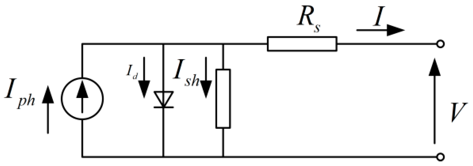
2.1. Photovoltaic (PV) Panel Model

Figure 1 shows the equivalent circuit of the PV cell. The basic equation that mathematically describes the I-V characteristic of the PV cell is given by Mutoh et al. [21]:
I = I p h I 0 { exp [ Q n k ( T + 273.15 ) ( V + I R s ) ] 1 } V + I R s R s h
where I and V represent the output current and voltage of the solar cell, respectively; I 0 is the reverse saturation current (in amperes) of the diode; I p h is the photocurrent (in amperes); n is a dimensionless junction material factor; Q is the electron charge ( 1.602 × 10 19 in coulombs); k is Boltzmann’s constant ( 1.38 × 10 23 in joules per kelvin); and T is the solar cell temperature (in degrees Celsius). An ideal PV cell has a very small equivalent series resistance R s and a very large equivalent parallel resistance R s h in the general engineering application [21]. Therefore, these two internal resistances R s and R s h can generally be neglected and Equation (1) is further simplified to
I = I p h I 0 { exp ( A 0 V ) 1 } I p h I 0 exp ( A 0 V )
where
A 0 = Q n k ( T + 273.15 )
The short-circuit current I s c and the open-circuit voltage V o c are used to change Equation (2) into
I s c = I p h , ( V = 0 , I = I s c )
I 0 = I s c exp ( A 0 V o c ) , ( V = V o c , I = 0 )
which describe two operating points in short and open circuits. The optimum operating points ( I m , V m ) that generate the maximum power is expressed using Equations (2)–(5) by Mutoh et al. [21]:
I m = I s c { 1 exp [ A 0 ( V m V o c ) ] }
A 0 = 1 V m V o c ln ( 1 I m I s c )
This means that Equation (7) can covert A 0 into a measurable quantity with the solar curve tracer. All of the parameters ( I s c , I m ,   V m , V o c ) are measured by the PV array manufacturer under standard conditions of solar irradiance ( S in watt per square meters) and temperature ( T ), which are 1000 W / m 2 and 25 ° C , respectively. A 0 represents a variable environmental parameter whose value is related to the variable parameters of the solar cell, T and S , but here it is a constant for the standard condition. Thus, using Equations (4) and (5), the output voltage V and power P are given by Equations (8) and (9) as a function of the output current I using circuit parameters I s c , V o c and A , respectively:
V = V o c [ 1 + 1 A ln ( 1 I I s c ) ]
P = I × V = I V o c [ 1 + 1 A ln ( 1 I I s c ) ]
where A = V o c V m V o c ln ( 1 I m I s c ) . For a PV system which consists of p series-connected PV panels. The subscript “i” could be used to represent the parameters of the ith solar cell under any environmental condition.
Defining the short-circuit current vector:
I s c = [ I s c 1 , I s c 2 , , I s c p ] , w h e r e I s c 1 < I s c 2 < < I s c p
The output voltage V s y s and power P s y s are given by Equations (11) and (12), respectively:
V s y s = V 1 + V 2 + + V p
P s y s = V s y s × I s y s = V 1 I s y s + V 2 I s y s + + V p I s y s = i p I V o c i [ 1 + 1 A i ln ( 1 I I s c i ) ] , where { I s c i 1 I < I s c i i = 1 , 2 p I s y s = I I s c 0 = 0
d P s y s d I = V o c i [ 1 + 1 A i ln ( 1 I I s c i ) ] + I V o c i 1 A i ( I I s c i ) + V o c i + 1 [ 1 + 1 A i + 1 ln ( 1 I I s c i + 1 ) ] + I V o c i + 1 1 A i + 1 ( I I s c i + 1 ) + + V o c p [ 1 + 1 A p ln ( 1 I I s c p ) ] + I V o c p 1 A p ( I I s c p )
where P s y s , V s y s , and I s y s are the output power, voltage, and current of PV system, respectively; I s c i is the ith short-circuit current of I s c . All parameters are constants except for P s y s and I s y s when both T i and S i are definite in Equation (12). Therefore, Equation (12) shows the theoretical relationship between output power P s y s and current I .
It should be noted that the values of parameters ( I s c , I m ,   V m , V o c ) are all given by the PV array manufacturer under standard conditions. By contrast, under nonstandard conditions, a new method should be studied for calculating those parameters. Under the engineering accuracy, the computational formulas of I s c i , I m i , V m i and V o c i are given by the following equations [40]:
I s c i = I s c × S i S r e f ( 1 + a Δ T i )
V o c i = V o c × ( 1 c Δ T i ) ln ( e + b Δ S i )
I m i = I m × S i S r e f ( 1 + a Δ T i )
V m i = V m × ( 1 c Δ T i ) ln ( e + b Δ S i )
where S r e f and T r e f are the solar irradiance and temperature under the standard condition, respectively; T i = T i T r e f ; S i = S i S r e f 1 ; the typical values of a, b, c are 0.0025/°C, 0.5 and 0.00288/°C, respectively.

2.2. Sufficient and Necessary Condition of Multiple-Peak

Figure 2 shows the location of bypass diodes in a PV array comprising p (p = 2) series connected PV array. I s c 1 and I s c 2 are matrix elements of I s c . Bypass diodes change the behavior of PV systems under PSC. When the current I smaller than the I s c of all PV array ( I <   I s c 1 ), the bypass diodes will not conduct (Figure 2b); when the current I is greater than the I s c of the ith PV array ( I >   I s c 1 ), the bypass diodes of ith PV array will conduct (Figure 2a). Therefore, the series circuits contain three operating modalities with the increasing of series current I . Figure 3 shows the P i I , V i I ,   P I characteristics of the PV array under the same solar cell temperature condition. The behaviors of PV systems under PSC are divided into two situations. In the first situation, I m 2 is greater than I s c 1 . The output behaviors of PV arrays are shown in Figure 3a.
Operating modality 1-1 ( 0 < I < I m 1 ): The values of the V 1 and V 2 remain approximately constant; P 1 and P 2 increase gradually, and the total power P s y s increase with the increase of I .
Operating modality 1-2 ( I m 1 I < I s c 1 ): The values of V 1 and P 1 decrease quickly; V 2 remains approximately constant; P 2 increases gradually with the increase of I . The value of d P s y s d I / I = I m 1 is greater than zero and d P s y s d I / I = I s c 1 is less than zero based on Equation (13). Meanwhile, Equation (12) is continuous; and the functions of P 1 and P 2 are monotonic in the range of I m 1 I s c 1 . So, there must exist a point which is named I p m a x 1 makes d P s y s d I equal to zero in the range of I m 1 - I s c 1 . The power at I p m a x 1 is named P m a x 1 , which is a local maximum power point.
Operating modality 1-3 ( I s c 1 I I s c 2 ): Then, the bypass diodes of 1th PV array conducts and the PV array is short–circuited; only PV array 2 keeps operating in the PV system. The values of V 1 and P 1 remain at zero. The characteristic of PV system is identical with array 2. The value of d P s y s d I / I = I m 2 is equal to zero at the point I m 2 , which is another local maximum power point (LMPP) current. I m 2 is defined with I p m a x 2 , corresponding to the local maximum power P m a x 2 .
In the second situation, I m 2 is smaller than I s c 1 . The output behaviors of PV arrays are shown in Figure 3b.
Operating modality 2-1 ( 0 < I < I m 1 ): The values of V 1 and V 2 remain approximately constant; P 1 and P 2 increase gradually, and the total power P s y s increases with the increase of I .
Operating modality 2-2 ( I m 1 I < I m 2 ): The values of V 1 and P 1 decrease slowly; V 2 remains approximately constant; P 2 increases gradually with the increase of I . The value of d P s y s d I / I = I m 1 is greater than zero and d P s y s d I / I = I m 2 is less than zero based on Equation (13). Meanwhile, Equation (12) is continuous; the functions of P 1 and P 2 are monotonic in the range of I m 1 I m 2 . So, there must exist a point which is named I p m a x make d P s y s d I equal to zero in the range of I m 1 - I m 2 .
Operating modality 2-3 ( I m 2 I I s c 2 ): The values of V 1 and P 1 decrease quickly in the range of I m 2 - I s c 1 ; V 2 and P 2 have the same behavior with V 1 and P 1 in the range of I m 2 I s c 2 . The bypass diodes of 1th PV array will conduct and the PV unit one is short–circuited when I I s c 1 . So, the output power of PV system P s y s always decreases with the increase of I in the range of I m 2 I s c 2 until it is equal to zero. There will not be a maximum power point (MPP) in the range of I m 2 I s c 2 .
To sum up, the PV systems have just one maximum power point when I m 2 is less than I s c 1 ; the PV system contains two local maximum power points when I m 2 is greater than I s c 1 . The sufficient and necessary condition of multiple-peak for the PV system is I s c 1 < I m 2 . This condition can be extended to the PV system which consists of p series-connected solar array and be expressed as:
I m i > I s c i 1
Substituting Equations (14) and (16) into Equation (18) gives:
I s c × S i 1 S r e f < I m × S i S r e f ( 1 + a Δ T i ) ( 1 + a Δ T i 1 )
where ( 1 + a T i ) ( 1 + a T i 1 ) 1 . Reorganizing Equation (19) gives:
S i S i 1 > I s c I m
Equation (20) defines the sufficient and necessary condition of multiple-peak for the PV system. Repeatedly operating Equation (20), the number of the LMPPs can be calculated, represented with q, and the S that meets it can be chosen to establish the irradiance vector:
S = [ S 1 , S 2 , , S q ] , w h e r e S 1 < S 2 < < S q
By using the MATLAB®/Simulink® (MathWorks, Natick, MA, USA) platform, the d p s y s d I I characteristic curves, based on Equation (13), can be illustrated in Figure 4. In the model of the solar cell, all constant values that are taken from the datasheet of XINYU/L-1260 are used to perform the simulation. Additionally, I s c , V o c , I m , and V m at standard conditions are 25.44 A, 66 V, 23.25 A, and 54.2 V, respectively. It can be seen from Figure 4a that there is just one MPP in the whole interval. Since of the S 2 / S 1 = 1.088 , which is less than I s c V m = 1.094 , the PV system in which two solar arrays are connected contains just one LMPP under PS condition. Figure 4b shows that the PV system appears two LMPPs, with S 2 increasing to 770 from 762; then, the S 2 / S 1 = 1.1 , which is greater than 1.094. Meanwhile, Figure 4c shows that there is just one MPP even when three solar arrays are connected in series, and the PV system has a complex PS condition. This further verifies that the partial shading condition is the necessary condition but not sufficient for multiple-peak. Meanwhile, the sufficient and necessary condition proposed in this paper could direct the choices of irradiance for simulations and experiments of GMPPT.
In engineering, I m I s c is roughly equivalent to 0.92 for the same type panels PV system [41]. Thus, the simplified sufficient and necessary condition of multiple-peak for a PV system with the same type panels can be expressed as:
S i S i 1 > 1.09
If we define the operating range of PV system, which consists of enough series-connected PV cells, the numbers of the local maximum power points are limited, which is decided by the range of irradiance. Table 1 shows the maximum numbers of LMPPs in different ranges of irradiance. Focusing on the LMPPs row of Table 1, the numbers of LMPPs are limited to 28 in the range of 100–1000. No matter how many PV arrays are series-connected there is only one maximum power point when S of all PV panels are greater than 920. The volume of LMPPs is increasing rapidly when S is less than 400. Thus, a powerful GMPPT algorithm is even more necessary under low solar irradiance conditions.

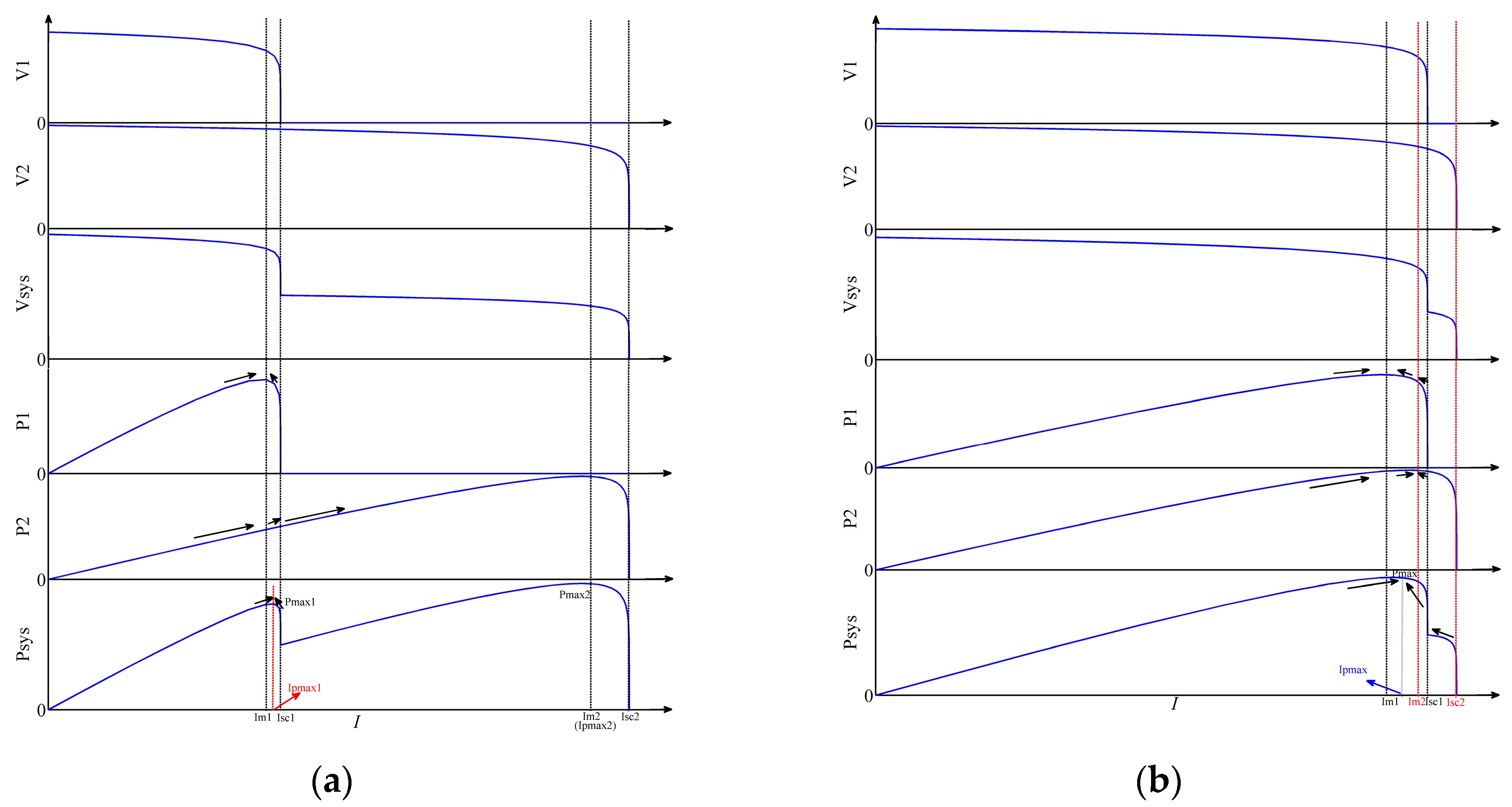
2.3. Zone of the Global Maximum Power Point (GMPP)

In Figure 3a, the P-I characteristic curves exist with two LMPPs which are P m a x 1 and P m a x 2 , respectively. The I p m a x 1 is almost equal to I m 1 . Since the solar array presents a constant voltage characteristic when the current I changes within smaller values, the V 2 almost equals V o c 2 at the point of I m 1 . Then, P m a x 1 and P m a x 2 can be expressed as:
P m a x 1 V m 1 × I m 1 + I m 1 × V o c 2
P m a x 2 = I m 2 × V m 2
It is assumed that P m a x 1 is larger than P m a x 2 ( P m a x 1 > P m a x 2 ).
I m 1 I m 2 > V m 2 V m 1 + V o c 2
Substituting Equations (15) and (17) into Equation (25) and ignoring the effect of the solar cell’s temperature gives:
S 1 S 2 > V m ln ( e + b Δ S 2 ) V m ln ( e + b Δ S 1 ) + V o c ln ( e + b Δ S 2 ) = L 1 , 2 2
where L 1 , 2 2 is dimensionless coefficient.
The error between ln ( e + b S 1 ) and ln ( e + b S 2 ) can be eliminated when S 1 and S 2 changing in the same order. Usually, V m / V o c is equal to 0.8 [41]. Rewriting Equation (26) gives:
L 1 , 2 2 0.44
Equation (27) is a simple expression of L 1 , 2 2 . The global maximum power point of PV system contains three possibilities. When S 1 S 2 > L 1 , 2 2 , the GMPPT is near I m 1 ; when S 1 S 2 < L 1 , 2 2 , the GMPPT is near I m 2 ; when S 1 S 2 = L 1 , 2 2 , the PV system contains two GMPPT near I m 1 and I m 2 , respectively.
Equation (26) can be extended to the PV system which contains q LMPPs and be expressed as:
S i S j > V m ln ( e + b Δ S j ) + V o c ln [ j + 1 q ( e + b Δ S j + 1 ) ] V m ln ( e + b Δ S i ) + V o c ln [ i + 1 q ( e + b Δ S i + 1 ) ] = L i , j q
The output power of PV system at I m i is larger than that at I m j when S i S j satisfies Equation (28). Repeatedly operating Equation (28), S finally meets it, represented as S m a x , and can be chosen to calculate the boundary of the GMPP zone, which is I s c m a x 1 I s c m a x , defining the current I and output power P s y s with I p m a x and P m a x at the GMPP, respectively. Obviously, I m m a x calculated with S m a x by Equation (16) can make the PV system output equal to approximately the global maximum power. That is to say that the I p m a x is nearly I m m a x .
Table 2 shows the typical values of L i , j q which ignore the effect of the ln ( e + b S j ) term in different LMPPs’ quantity conditions. Focusing on the typical values of the L i , j q column, the probability of the traditional MPPT method, such as incremental conductance (INC) algorithm and perturbation and observation (P&O) algorithm, can find the GMPPT is about 44.4% under the two LMPPs condition, and 28.5% under the three LMPPs condition. It decreases to 21% under the four 4 LMPPs condition. The probability decreases rapidly with an increase in the quantity of LMPPs, but it still exist. This is to say the traditional methods have some adaptability for GMPPT control. This feature is beneficial to GMPPT. However, it is not conducive to the planning of the experimental program.

2.4. Relationship between S and Operating Parameters

There are many MPPT control methods adopting irradiance and temperature as the parameters to calculate the control reference signal [37,38,39]. However, all of them obtain the parameters by using irradiance and temperature sensors. On the one hand, the irradiance cannot be measured accurately under PSC. On the other hand, the measurement error of the sensors brings a lot of uncertainty even in normal environmental conditions. Moreover, the application of the sensors increases the cost of the system. Therefore, it is necessary to establish a relation between irradiance and the output current & voltage of solar arrays in any operation status.
In the PV system, the solar cell’s running state is described by its output voltage V and current I . The expression is given by Mutoh et al. [21]:
I = I s c { 1 exp ( A ) [ exp ( A V / V o c ) 1 ] }
V and I are measured in real time in the operation process of PV system. Equation (29) can be regarded as a function of A , I s c and V o c . The relationship between S and T is expressed as [42]:
T = T a i r + 0.02 × S
Rewriting the Equation (29) gives:
f ( S ) = I s c { 1 exp ( A ) [ exp ( A V / V o c ) 1 ] } I = I s c S S r e f [ 1 + a ( 0.02 S + T a i r ) a T r e f ] { 1 e x p [ A ( V V o c [ 1 c ( 0.02 S + T a i r ) + c T r e f ] ln ( e + b S S r e f b ) 1 ) ] + e x p ( A ) } I
d f ( S ) d S = { I s c 1 S r e f [ 1 + a ( 0.02 S + T a i r ) a T r e f ] + I s c S S r e f 0.02 a } { 1 e x p [ A ( V V o c [ 1 c ( 0.02 S + T a i r ) + c T r e f ] ln ( e + b S / S r e f b ) 1 ) ] + e x p ( A ) } + I s c b S / S r e f [ 1 + a ( 0.02 S + T a i r ) a T r e f ] { e x p [ A ( V V o c [ 1 c ( 0.02 S + T a i r ) + c T r e f ] ln ( e + b S / S r e f b ) 1 ) ] } V A V o c { [ 1 c ( 0.02 S + T a i r ) + c T r e f ] ln ( e + b S / S r e f b ) } 2 { c 0.02 ln ( e + b S / S r e f b ) + [ 1 c ( 0.02 S + T a i r ) + c T r e f ] b / S r e f e + b S / S r e f b }
Define M ( S ) = c × 0.02 ln ( e + b S / S r e f b ) + [ 1 c ( 0.02 S + T a i r ) + c T r e f ] b / S r e f e + b S / S r e f b .
  M ( S ) > c × 0.02 + [ 1 c ( 0.02 S + T a i r ) + c T r e f ] b / S r e f e + b S / S r e f b > 0 . 02 c + [ 1 c 70 + c 25 ] b / 1000 e > 0
Equation (31) defines the relationship between S , V and I . It is easily to prove, strictly, that the d f ( S ) d S constant is greater than zero when S is in the range of 0–1000. Thus, there is only one value of S to make f ( S ) = 0 , which can be solved quickly by the Newton iteration method in the process of actual calculation. Based on the nonlinear relation, the irradiance of solar array absorption can be calculated in real-time.

2.5. Relationship between I p m a x i and Environment Parameters

According to Equation (12), to solve the maximum value of output power P m a x , Equation (33) can be given:
d P s y s d I = 0
Substituting Equation (13) into Equation (33) gives:
d P s y s d I = V o c i [ 1 + 1 A i ln ( 1 I I s c i ) ] + I V o c i 1 A i ( I I s c i ) + V o c i + 1 [ 1 + 1 A i + 1 ln ( 1 I I s c i + 1 ) ] + I V o c i + 1 1 A i + 1 ( I I s c i + 1 ) + + V o c p [ 1 + 1 A p ln ( 1 I I s c p ) ] + I V o c p 1 A p ( I I s c p ) = 0
Reorganizing Equation (34) gives:
V o c i A i I s c i ( I s c i I ) + V o c i A i ln I s c i ( I s c i I ) + + V o c p A p I s c p ( I s c p I ) + V o c p A p ln I s c p ( I s c p I ) = V o c i + V o c i A i + + V o c p + V o c p A p
The Euler’s Number as the base for the exponential operation on both sides of the equation and reorganizing Equation (35) gives:
{ [ exp I s c i ( I s c i I ) ] V o c i A i I s c i ( I s c i I ) V o c i A i } { [ exp I s c p ( I s c p I ) ] V o c p A p I s c p ( I s c p I ) V o c p A p } = { exp V o c i ( 1 + 1 A i ) } { exp V o c p ( 1 + 1 A p ) }
Rewriting Equation (36) gives:
i p ( I s c i I s c i I exp I s c i I s c i I ) V o c i A i = i p exp V o c i ( 1 + 1 A i )
Therefore, Equation (37) shows the indirect relationship between output current I s y s at MPP and environmental parameters S i and T i . It is a piecewise transcendental equation, which can be solved quickly by the Newton iteration method in the process of actual calculation. The solutions of Equation (37) are represented by I p m a x i , which contain all possible local maximum power point current values. Namely, the solar generation system will operate at GMPP when the output current I equals to the optimum solution of Equation (37), which is one of the possible values of I p m a x i and represents with I p m a x . I p m a x can be solved quickly using the information of the GMPP zone, which is identified in Section 2.3. It should be noted that the values of parameters ( I s c , I m ,   V m , V o c ) are all given by the PV array manufacturer under standard conditions. Under non-standard conditions, the four parameters can be easily calculated by using Equations (14)–(17) with standard parameters, which are provided by the PV array manufacturer, and environment parameters S i and T i , which are calculated by Equations (30) and (31).

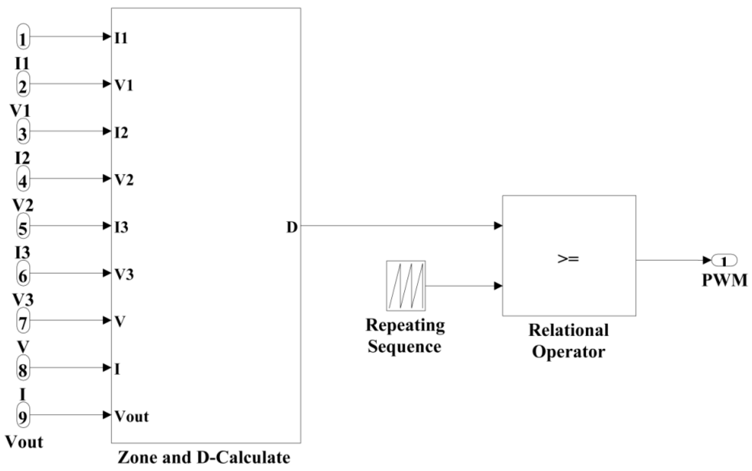
3. Proposed GMPPT Control Strategy

From the engineering cybernetics perspective, the ultimate goal of GMPPT is to control the output current of the solar panels to reach I p m a x accurately and rapidly. The traditional method based on INC and P&O have their greatest use in engineering because of the stronger robustness and adaptability. However, the aforementioned traditional MPPTs are not able to identify the GMPP from the LMPPs when the PV characteristic curve consists of more than one peak. From an engineering cybernetic perspective, the fundamental cause of these traditional MPPT methods tend to converge to the first peak is the algorithms’ operation initial value always is settled to the near of it. In order to achieve the GMPP, the OIV of the algorithms should be settled within the GMPP range or near the I p m a x   when PSC with multiple-peak occurs. Due to I p m a x and I m m a x locating in the same zone, the expression is simpler than I p m a x . In this work, the proposed control strategy adopts I m m a x directly as the OIV of INC to make the INC method achieve GMPP control. It should be pointed out that the proposed method will have better performance when I p m a x is chosen as the OIV of INC in a medium number of PV arrays in series. In large numbers of PV arrays in series, the proposed method adopting I m m a x has more advantages than I p m a x .
The control procedures cited above are summarized in the flowchart shown in Figure 5. According to the proposed algorithm, as shown in blocks 1 and 2 (B-1 and B-2), the voltage current of the solar cell and PV system, and the temperature of air are measured. The irradiances and temperatures of every solar cell obtained are calculated using the functions shown in Equations (30) and (31) (B-3). The vector S , which removes the elements unsatisfied the Equation (22), can be structured and the numbers of LMPPs are calculated (B-4). Based on the Equation (28), the zone of GMPP can be identified, the “max” at B-5 represents the S m a x and S m a x 1 in S , which will be taken to calculate the I m m a x , I s c m a x and I s c m a x 1 (B-5). The values of I m m a x are stored (B-6). Therefore, the current at the GMPP is within the zone between I s c m a x 1 and I s c m a x . If I is greater than a critical value I s c m a x 1 and less than an upper limit value I s c m a x (B-7), by using the INC with small step, the operating point is adjusted to the GMPP (B-8). Otherwise, output I to make the I change towards the GMPP zone rapidly (B-9), until it is within the GMPP zone.
The INC method is used extensively because of its rapidly, high-tracking accuracy at a steady state, its flexibility to adapt to rapidly changing environmental conditions, and simplicity in application. Meanwhile, the INC method can be used instead of other traditional methods in the proposed method to improve performance.
The whole proposed method includes only three subsets: Calculate, Select and Compare. Consequently, we can draw the following three conclusions:
(1)
When I is outside of the zone of I s c m a x 1 - I s c m a x , the error between I m m a x and I is large (i.e., the operating point is far from the GMPP), the change in the duty cycle is large, and it reaches the GMPP zone rapidly.
(2)
When I is within the zone of I s c m a x 1 - I s c m a x which is narrowly bound (i.e., the operating point is near GMPP), the INC method with small step is adopted to make the operating point approach the GMPP rapidly and accurately. Then, the change in the duty cycle is small to avoid the oscillation at GMPP.
(3)
When the environmental conditions change and the zone of I s c m a x 1 - I s c m a x goes with it, if   I is still within the new zone of GMPP (B-7), the INC method will find the GMPP actively, rapidly and accurately (B-8). If I is outside of the new zone of the GMPP, the change in the duty cycle is large, and reaches the GMPP zone rapidly (B-9). Namely, the proposed GMPPT control method has stronger robustness and adaptability.
Thus, this GMPPT control method can be called the “GMPPT method based on optimal initial value incremental conductance control (OIV-INC)”.

4. Results and Discussion

4.1. Experiment for Calculating S

One of the key points of the GMPPT method proposed in this paper is to obtain environmental parameters S without the irradiance sensor. To investigate the effectiveness and accuracy of the calculating method in Section 2.4, several experiments were designed using real environmental parameters measurement system of PV panels, as illustrated in Figure 6. The whole experimental system consists of 10 KVA PV systems, irradiance and temperature measuring instrument (FZD-R4-2000), power analyzer (Fluke NORMA 4000) and a personal computer.
The data from measurement and calculations are shown in Table 3. Actual measurement data are collected at Tianjin, China for a sunny from 11 a.m. to 3 p.m., and some experimental data in [43] are also introduced to support the discussion.
Tair represents the environmental temperature; V and I represent the voltage and current at any operating point of PV array; S and S* are the solar irradiance by measurement and calculation, respectively; Ipmax and Vm are the current and voltage at GMPP of PV array, respectively. For ease of analysis, the data of V and I are taken from near the maximum power point. It can be seen from I and Ipmax columns that the current value Ipmax is approximately equal to the corresponding value I and the average error between Ipmax and I is −0.0193 which less than 4% of I. Since the Ipmax is calculated by using S, the average error value represents the error between the S and S*. Focusing on the S and S* columns, we can find that the average error between S and S* is less 3.7% of S which is in concordance with the aforementioned average error, and it satisfies the request of the engineers. For the diversity of experimental data sources, some data from [43] are taken in this paper. The data from [43] do not give the environmental temperature, assuming it to be 4 °C because the data were collected in December 2013 in Nanjing, China. By comparing Ipmax with I, we can see that the data by using the [43] have the same average error level. Meanwhile, the result also shows that Tair has a negligible effect on the calculation of S, which is beneficial for the engineering application.

4.2. Analysis and Discussion of the Simulation Results

In order to evaluate the performance of the proposed method under different weather conditions, a PV system includes three solar panels, a DC-DC boost converter which is selected according to load requirements [44], a load and a control system that are considered and simulated on a MATLAB®/Simulink® platform.
The Simulink model of the PV system with the proposed method is shown in Figure 7. Figure 8 shows a Simulink/SimPower subsystem model of one PV panel module; I1 and V1 represent the operation current and voltage of the PV model 1 in Figure 7, respectively. Figure 9 describes the subsystem model of the proposed GMPPT controller, which includes the calculation block for GMPP zone and duty cycle D, which is based on the flowchart shown in Figure 6, and the control logic block which produces the PWM signal. In the MATLAB® model of the solar cell, I s c , V o c , I m and V m are the same as in Section 2.2 at standard conditions. The inductance and the capacitor of the boost DC/DC converter are the ideal components; the snubber resistance, internal resistance and forward voltage of the diode are 500   Ω , 0.001   Ω and 0.8   V , respectively; insulated gate bipolar transistor (IGBT) with the 0.001 Ω internal resistance and a 105 Ω snubber resistance is chosen as the switch; the load resistance is 500 Ω . Other parameters such as R 1 , L , C and C 1 are 1   Ω , 0.01   H , 2 mF and 2 mF , respectively.
To evaluate the performance of the proposed GMPPT method different parameters are considered, such as the response time, the static error and the tracking efficiency. As discussed in [45,46], the tracking efficiency is an important parameter for the assessment of an MPPT algorithm. The MPPT behavior can be analyzed both in static and dynamic conditions [47]. The static MPPT efficiency describes the ability of an MPPT to find and track the desired MPP under constant environmental conditions. A stabilization period is necessary for the evaluation of the static MPPT efficiency [48]. In the steady state, the static MPPT efficiency can be defined as:
η p v ( t ) = P M P P T ( t ) P m a x ( t )
where P M P P T ( t ) is the output power of the PV system under the control of the MPPT, whereas P m a x ( t ) represents the true maximum output power.
In the case of variable partially shaded conditions, the static efficiency cannot provide a sufficient degree of precision about the MPP tracking. Therefore, the dynamic MPPT efficiency has to be considered. It describes the ability in tracking the desired MPP in the case of variable environmental conditions and it can be determined as the average ratio between P M P P T ( t ) and P m a x ( t ) over a desired time interval. The dynamic MPPT efficiency can be defined as:
η p v = 0 t P M P P T ( t ) d t 0 t P m a x ( t ) d t = E M P P T E m a x
where the E M P P T is the output energy of the PV system using the MPPT method; E m a x represents the true maximum output energy.
The scanning method can find the global MPP under any conditions, so it can be used as the standard for comparison. To show the effectiveness of the developed MPPT method, a performance comparison between the proposed method and the scanning MPPT algorithm recently published by [27] is presented in the following.

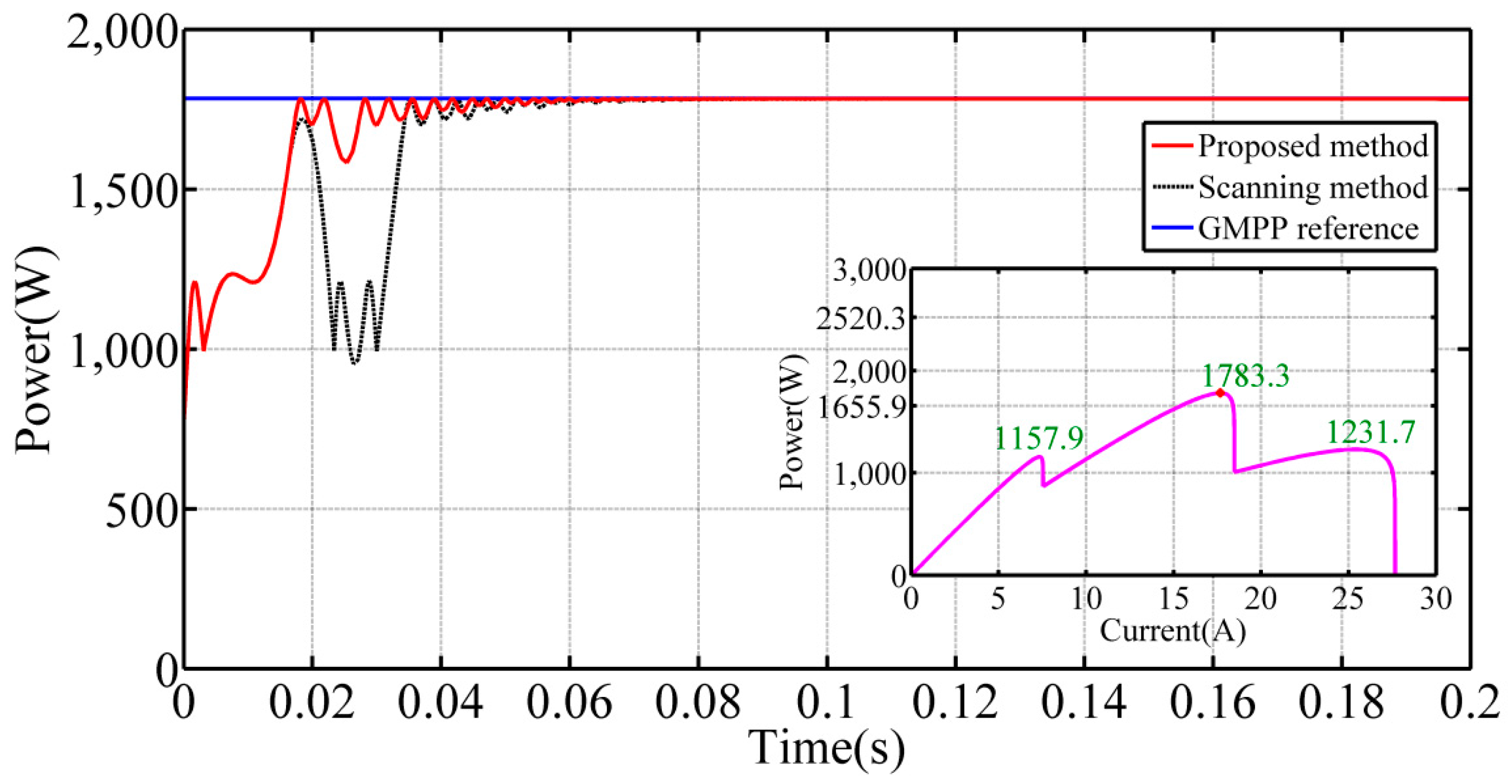
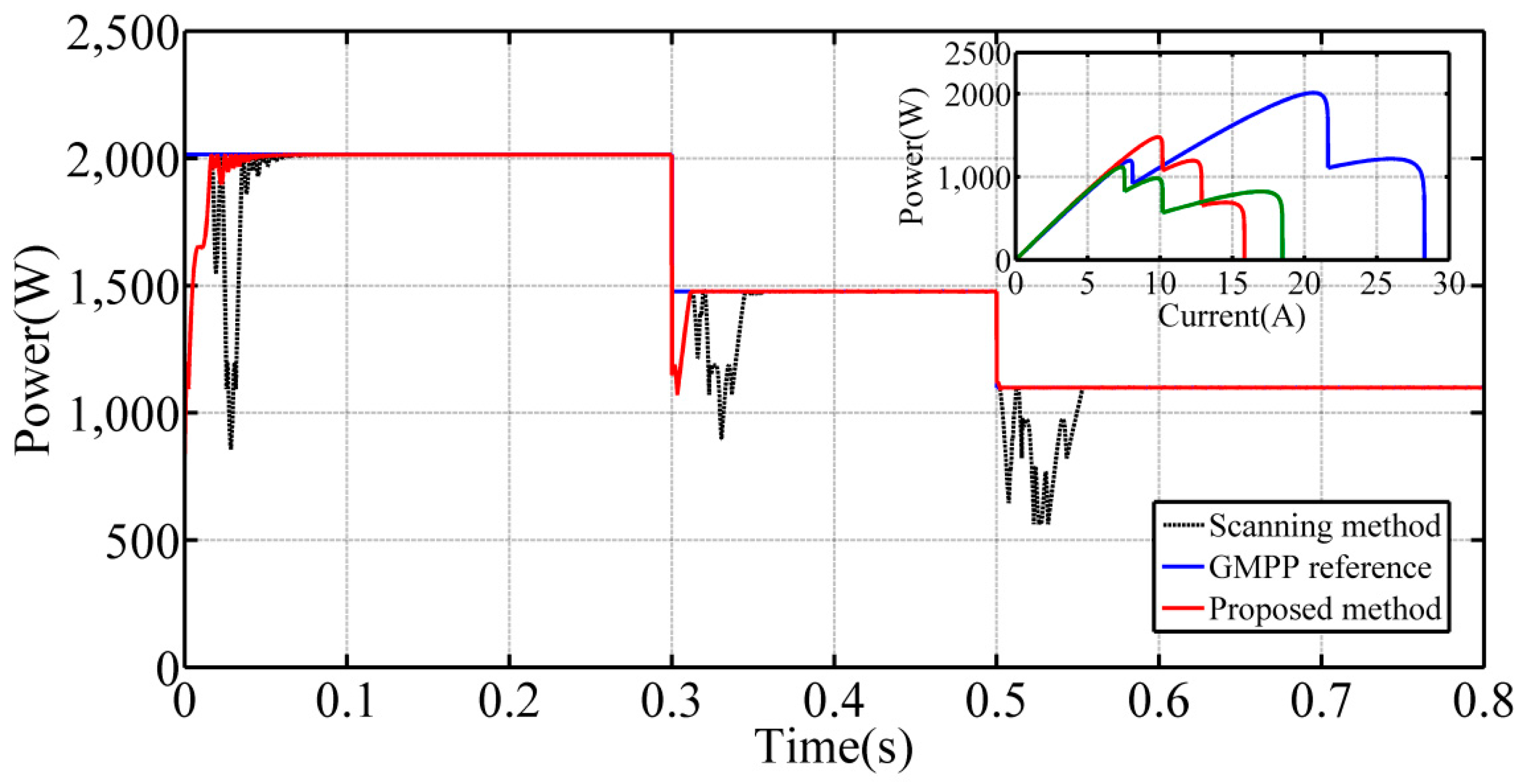
4.2.1. Partial Shading Condition

This investigation is implemented to assess and compare the performance of the scanning method under partial shading conditions. The solar irradiance and the solar array temperature are considered 1000 W/m2 and 25 °C, respectively. One shaded cell receives an insolation of 400 W/m2 and a temperature of 15 °C. The MPPT trajectories for OIV-INC and the scanning algorithms are shown in Figure 10. In the range of 0 to 0.02 s, the proposed method finds the GMPP zone rapidly and controls the output current of the PV system towards the GMPP. After 0.02 s, the PV system is operating into steady state. From the output P-I characteristic curve of the PV generator depicted in Figure 10, two power peaks are observed corresponding, respectively, to the GMPP (2520.3 W) and the LMPP (1655.9 W). Figure 10 shows that both of the two methods find the local MPP at about 0.01 s; the output power keeps increasing after 0.01 s up to the maximum power at about 0.018 s. After 0.018 s, the output power remains near the GMPP by using the proposed method. The scanning method finishes the scanning process at 0.02 s, and then controls the PV system operating towards the GMPP. As this figure shows, it is obvious that both of the two methods can find the global MPP in this condition. OIV-INC, in comparison with the scanning method, has the same accuracy, but a better time response.
For an extensive verification, initially, three different insolation and temperature levels are applied to the PV system, which are set to 1000 W/m2 and 60 °C, 700 W/m2 and 40 °C, 300 W/m2 and 20 °C, and simulation results are repeated. From the output P-I characteristic curve of the PV generator depicted in Figure 11, three power peaks are observed corresponding, respectively, to GMPP (1783.3 W), the LMPP1 (1157.9 W) and LMPP2 (1231.7 W). The MPPT trajectories for OIV-INC and the scanning algorithms are shown in Figure 11. As this figure shows, it is obvious that both of the two methods can find the global MPP in this condition. Figure 11 shows the similar dynamic characteristics with Figure 10 by using the proposed method. It should be noted that the dynamic characteristic is becoming poor by using the scanning method with the increase of the number of GMPPs in the PV system. In addition, the OIV-INC algorithm has the same accuracy and better response time in comparison with the scanning algorithm. Furthermore, it can be noticed that the proposed GMPPT method is able to reach and track the GMPP with a static efficiency of 99.98% when time in the range of 0.04–0.2 s. By using Equation (39), a dynamic MPPT efficiency of 96.86% has been achieved based on the OIV-INC method, and the efficiency is much higher than that of the scanning method, by 2.01%.

4.2.2. Fast Variations of the Solar Array Temperature and Solar Irradiance as Well as Partial Shading Conditions

To investigate and verify the performance and accuracy of the proposed OIV-INC method under rapidly changing solar cell temperatures and the solar irradiances, two step changes, globally, are applied to the solar cell temperature and the solar irradiance, as represented in Figure 12, which is used for the first solar array. The same step change is applied to the temperature and irradiance of the other two shaded cells, as represented in Figure 13. The output power trajectories of solar arrays for OIV-INC and scanning methods are plotted in Figure 14. From the output P-I characteristic curves of the PV generator depicted in Figure 14, two power peaks are always observed corresponding, respectively, to different operating times. Globally, the P-I characteristic curve has six power peaks. The step change occurs at 0.3 s and 0.5 s in Figure 14, then the control system detects that the environmental conditions have been changed based on the proposed method; the operating current I is outside of the GMPP zone and the control system outputs the error between I and I m m a x directly to make the I move to the GMPP zone rapidly. Therefore, as Figure 14 shows, the power characteristic curves present a better dynamic feature when step change occurs. The proposed GMPPT method has the ability to identify the true peak (GMPP) among the multiple local peaks (LMPPs).
For an extensive verification, initially, three different insolation and temperature levels are applied to the PV system, which are shown in Figure 12, Figure 13 and Figure 15, and simulation results are repeated. Figure 16 shows the output power trajectories of solar arrays for OIV-INC and the scanning method. From the output P-I characteristic curves of the PV generator depicted in Figure 16, there are always three power peaks observed corresponding, respectively, to different operating times. Globally, the P-I characteristic curve has nine power peaks. Focusing the range of 0–0.3 s in Figure 16, the power trajectories based on the proposed method pass the first LMPP at about 0.01 s and run into the GMPP zone, find and remain at the GMPP at about 0.02 s. The step change occurs at 0.3 s, and then the whole PV system operates in the short-circuit condition; the operating current I is outside of the GMPP zone; the control system outputs the error between I and I m m a x directly to make the I pass two LMPPs and moving to the GMPP zone rapidly. Therefore, as Figure 14 shows, the power trajectories in Figure 16 present a better dynamic feature when step change occurs. Still, the proposed GMPPT method can find the true peak (GMPP) rapidly and accurately among the multiple local peaks (LMPPs).
To evaluate the performance of the proposed OIV-INC MPPT algorithm, the dynamic MPPT efficiency can be calculated which are shown in Table 4 by using Equation (39).
Focusing on the η O I V I N C row of Table 4, η O I V I N C are 99.15% and 99.01%, corresponding to Figure 14 and Figure 16 globally, respectively. When time in the range of 0.5–0.8 s, η O I V I N C are 99.58% and 99.609%, corresponding to Figure 14 and Figure 16, respectively. From Table 4, the dynamic efficiency of the solar arrays can reach 99% in the whole stage and in different operating periods. The calculated results show that approximately 2.8% of the solar energy is output when using the proposed method more than the scanning algorithm in global. The scanning method frequently starts to find the GMPP when the environment condition changes continuously, which will cause a loss in power. Then, the advantage of the proposed method is especially obvious.
From the Figure 10, Figure 11, Figure 14 and Figure 16, the simulation results show that the proposed OIV-INC GMPP method can find the true peak (GMPP) rapidly among the multiple local peaks (LMPPs). Moreover, the OIV-INC GMPP method has adequate accuracy under partial shading conditions. In addition, the setting time of the output power is less than 0.04 s. At steady-state, the output curves are non-vibrating and the efficiency is maintained at a high level under all conditions.

5. Conclusions

A detailed analysis of the series PV arrays’ dynamic performance and the design of a GMPPT solution have been introduced in this paper. The sufficient and necessary condition of multiple-peak is present under PSC; the principles of judgment for the number of the peak points and the zone of the GMPP are established. Based on the principles, the search zone is identified, and simultaneously, the boundary of the zone is expressed by mathematical formula. For getting the environmental parameters without the irradiance sensor, a definable nonlinear relation has been built in this paper between irradiance and the output current & voltage of solar arrays in any operation status. Meanwhile, this paper builds the unified nonlinear relation between variable parameters and the output current at LMPPs, one of which can be settled as the initial value of the INC to achieve the GMPP. The proposed method can track the GMPP under all changing climate conditions rapidly and accurately. In this work, the INC method is used also can increase the steady-state performance and the robustness when the PSC continuous slow change. Meanwhile, the simplicity of implementation, high GMPPT accuracy, and high efficiency level are the additional advantages. A numerical analysis has been performed by using the scanning method as a benchmark reference MPPT technique. The numerical results confirm the validity of the proposed method because the performances of OIV-INC are always better with respect to the corresponding performances obtainable by adopting the scanning algorithm.

Acknowledgments

This work was supported by National Natural Science foundation of China (NO. 50877053) and Natural Science Foundation of Tianjin of China (NO. 09JCYBJC07100).

Author Contributions

The authors participated at the paper through a wide and balanced cooperation. They all worked at the mathematical model, the simulation set-up, the experiments and writing the manuscript. They have given equal contribution regarding all aspects of the paper.

Conflicts of Interest

The authors declare no conflict of interest.

Nomenclature

PVPhotovoltaic
GMPPTGlobal Maximum Power Point Tracking
LMPPLocal Maximum Power Point
MPPMaximum Power Point
PSCPartial Shading Condition
INCIncremental Conductance
OIVOperation Initial Value
OIV-INCOptimal Initial Value Incremental Conductance

References

  1. De Brito, M.A.G.; Galotto, L.; Sampaio, L.P.; de Azevedo e Melo, G.; Canesin, C.A. Evaluation of the main MPPT techniques for photovoltaic applications. IEEE Trans. Ind. Electron. 2013, 60, 1156–1167. [Google Scholar] [CrossRef]
  2. Seyedmahmoudian, M.; Horan, B.; Rahmani, R.; Oo, A.M.T.; Stojcevski, A. Efficient photovoltaic system maximum power point tracking using a new technique. Energies 2016, 9, 147. [Google Scholar] [CrossRef]
  3. Sullivan, C.R.; Awerbuch, J.J.; Latham, A.M. Decrease in photovoltaic power output from ripple: Simple general calculation and the effect of partial shading. IEEE Trans. Power Electron. 2013, 28, 740–747. [Google Scholar] [CrossRef]
  4. Piegari, L.; Rizzo, R.; Spina, I.; Tricoli, P. Optimized adaptive perturb and observe maximum power point tracking control for photovoltaic generation. Energies 2015, 8, 3418–3436. [Google Scholar] [CrossRef]
  5. Lee, J.-S.; Lee, K.B. Variable DC-link voltage algorithm with a wide range of maximum power point tracking for a two-string PV system. Energies 2013, 6, 58–78. [Google Scholar] [CrossRef]
  6. Yau, H.T.; Wu, C.H. Comparison of extremum-seeking control techniques for maximum power point tracking in photovoltaic systems. Energies 2011, 4, 2180–2195. [Google Scholar] [CrossRef]
  7. Wasynczuk, O. Dynamic behavior of a class of photovoltaic power systems. IEEE Trans. Power Appar. Syst. 1983, 9, 3031–3037. [Google Scholar] [CrossRef]
  8. Teulings, W.J.A.; Marpinard, J.C.; Capel, A.; O’Sullivan, D. A new maximum power point tracking system. In Proceedings of the 24th Annual IEEE Power Electronics Specialists Conference, Seattle, WA, USA, 20–24 June 1993; pp. 833–838.
  9. Femia, N.; Petrone, G.; Spagnuolo, G.; Vitelli, M. Optimization of perturb and observe maximum power point tracking method. IEEE Trans. Power Electron. 2005, 20, 963–973. [Google Scholar] [CrossRef]
  10. Yang, B.; Li, W.; Zhao, Y.; He, X. Design and analysis of a grid connected photovoltaic power system. IEEE Trans. Power Electron. 2010, 25, 992–1000. [Google Scholar] [CrossRef]
  11. Zegaoui, A.; Aillerie, M.; Petit, P.; Sawicki, J.P.; Charles, J.P.; Belarbi, A.W. Dynamic behavior of PV generator trackers under irradiation and temperature changes. Sol. Energy 2011, 85, 2953–2964. [Google Scholar] [CrossRef]
  12. Petrone, G.; Spagnuolo, G.; Vitelli, M. A multivariable perturb-and-observe maximum power point tracking technique applied to a single-stage photovoltaic inverter. IEEE Trans. Ind. Electron. 2011, 58, 76–84. [Google Scholar] [CrossRef]
  13. Xiao, W.; Dunford, W.G. A Modified Adaptive hill climbing MPPT Method for photovoltaic power systems. In Proceedings of the Power Electronics specialists Conference, Aachen, Germany, 20–25 June 2004; pp. 1957–1963.
  14. Salas, V.; Barrado, A. Review of the maximum power point tracking algorithms for stand-alone photovoltaic systems. Sol. Energy Mater. Sol. Cells 2006, 90, 1555–1578. [Google Scholar] [CrossRef]
  15. Liu, F.; Duan, S.; Liu, F.; Liu, B.; Kang, Y. A variable step size INC MPPT method for PV systems. IEEE Trans. Ind. Electron. 2008, 55, 2622–2628. [Google Scholar]
  16. Zhou, X.; Song, D.; Ma, Y.; Chen, D. The simulation and design for MPPT of PV system based on incremental conductance method. In Proceedings of the 2010 WASE International Conference on Information Engineering (ICIE), Beidaihe, China, 14–15 August 2010; pp. 314–317.
  17. Kish, G.J.; Lee, J.J.; Lehn, P.W. Modeling and control of photovoltaic panels utilizing the incremental conductance method for maximum power point tracking. IET Renew. Power Gener. 2012, 6, 259–266. [Google Scholar] [CrossRef]
  18. Chaouachi, A.; Kamel, R.M.; Nagasaka, K. A novel multi-model neuro-fuzzy-based MPPT for three-phase grid-connected photovoltaic system. Sol. Energy 2010, 84, 2219–2229. [Google Scholar] [CrossRef]
  19. Messai, A.; Mellit, A.; Guessoum, A.; Kalogirou, S.A. Maximum power point tracking using a GA optimized fuzzy logic controller and its FPGA implementation. Sol. Energy 2011, 85, 265–277. [Google Scholar] [CrossRef]
  20. Rajesh, R.; Mabel, M.C. Efficiency analysis of a multi-fuzzy logic controller for the determination of operating points in a PV system. Sol. Energy 2014, 99, 77–87. [Google Scholar] [CrossRef]
  21. Mutoh, N.; Ohno, M.; Inoue, T. A method for MPPT control while searching for parameters corresponding to weather conditions for PV generation systems. IEEE Trans. Ind. Electron. 2006, 53, 1055–1065. [Google Scholar] [CrossRef]
  22. Zhao, J.; Zhou, X.; Ma, Y.; Liu, W. A novel maximum power point tracking strategy based on optimal voltage control for photovoltaic systems under variable environmental conditions. Sol. Energy 2015, 122, 640–649. [Google Scholar] [CrossRef]
  23. Salam, Z.; Ahmed, J.; Merugu, B.S. The application of soft computing methods for MPPT of PV system: A technological and status review. Appl. Energy 2013, 107, 135–148. [Google Scholar] [CrossRef]
  24. Patel, H.; Agarwal, V. Maximum power point tracking scheme for PV systems operating under partially shaded conditions. IEEE Trans. Ind. Electron. 2008, 55, 1689–1698. [Google Scholar] [CrossRef]
  25. Anula, K.; Saroj, R. A review of particle swarm optimization and its applications in solar photovoltaic system. Appl. Soft Comput. 2013, 13, 2997–3006. [Google Scholar]
  26. Liu, Y.; Liu, C.; Huang, J.; Chen, J. Neural-network based maximum power point tracking methods for photovoltaic systems operating under fast changing environments. Sol. Energy 2013, 89, 42–53. [Google Scholar] [CrossRef]
  27. Kotti, R.; Shireen, W. Efficient MPPT control for PV systems adaptive to fast changing irradiation and partial shading conditions. Sol. Energy 2015, 114, 397–407. [Google Scholar] [CrossRef]
  28. Seyedmahmoudian, M.; Mekhilef, S.; Rahmani, R.; Yusof, R.; Shojaei, A.A. Maximum power point tracking of partial shaded photovoltaic array using an evolutionary algorithm: A particle swarm optimization technique. J. Renew. Sustain. Energy 2014, 6. [Google Scholar] [CrossRef]
  29. Seyedmahmoudian, M.; Rahmani, R.; Mekhilef, S.; Than Oo, A.M.; Stojcevski, A.; Tey Kok, S. Simulation and hardware implementation of new maximum power point tracking technique for partially shaded PV system using hybrid DEPSO method. IEEE Trans. Sustain. Energy 2015, 6, 850–862. [Google Scholar] [CrossRef]
  30. Seyedmahmoudian, M.; Horan, B.; Soon, T.K.; Rahmani, R.; Than Oo, A.M.; Mekhilef, S. State of the art artificial intelligence-based MPPT techniques for mitigating partial shading effects on PV systems—A review. Renew. Sustain. Energy Rev. 2016, 64, 435–455. [Google Scholar] [CrossRef]
  31. Raja, B.; Kumar, M.R.S.; Vikash, S.; Hariharan, K. Maximum power point tracking in solar panels under partial shading condition using equilibration algorithm. In Proceedings of the International Conference on Communication and Signal Processing, Melmaruvathur, India, 6–8 April 2016; pp. 2073–2077.
  32. Alajmi, B.N.; Ahmed, K.H.; Finney, S.J.; William, B.W. A maximum power point tracking technique for partially shaded photovoltaic systems in Microgrids. IEEE Trans. Ind. Electron. 2013, 60, 1596–1606. [Google Scholar] [CrossRef]
  33. Manganiello, P.; Balato, M.; Vitelli, M. A survey on mismatching and aging of pv modules: The closed loop. IEEE Trans. Ind. Electron. 2015, 62, 7276–7286. [Google Scholar] [CrossRef]
  34. Balato, M.; Costanzo, L.; Vitelli, M. Reconfiguration of PV modules: A tool to get the best compromise between maximization of the extracted power and minimization of localized heating phenomena. Sol. Energy 2016, 138, 105–118. [Google Scholar] [CrossRef]
  35. Balato, M.; Costanzo, L.; Vitelli, M. Series-parallel PV array re-configuration: Maximization of the extraction of energy and much more. Appl. Energy 2015, 159, 145–160. [Google Scholar] [CrossRef]
  36. Bratcu, A.I.; Munteanu, I.; Bacha, S.; Picault, D.; Raison, B. Cascaded DC-DC converter photovoltaic systems: Power optimization issues. IEEE Trans. Ind. Electron. 2011, 58, 403–411. [Google Scholar] [CrossRef]
  37. Gao, X.; Li, S.; Gong, R. Maximum power point tracking control strategies with variable weather parameters for photovoltaic generation systems. Sol. Energy 2013, 93, 357–367. [Google Scholar] [CrossRef]
  38. Li, S.; Gao, X.; Wang, L.; Liu, S. A novel maximum power point tracking control method with variable weather parameters for photovoltaic systems. Sol. Energy 2013, 97, 529–536. [Google Scholar] [CrossRef]
  39. Li, S. A MPPT control strategy with variable weather parameter and no DC/DC converter for photovoltaic systems. Sol. Energy 2014, 108, 117–125. [Google Scholar] [CrossRef]
  40. Su, J.; Yu, S.; Zhao, W. Investigation on engineering analytical model of silicon solar cells. Acta Energiae Sol. Sin. 2001, 22, 409–412. [Google Scholar]
  41. Hajighorbani, S.; Radzi, M.A.M.; Kadir, M.Z.A.A.; Shafie, S.; Zainuri, M.A.A.M. Implementing a novel hybrid maximum power point tracking technique in DSP via Simulink/MATLAB under partially shaded conditions. Energies 2016, 9. [Google Scholar] [CrossRef]
  42. Salameh, Z.M.; Borowy, B.S.; Amin Atia, R.A. Photovoltaic module-site matching based on the capacity factors. IEEE Trans. Energy Convers. 1995, 10, 326–332. [Google Scholar] [CrossRef]
  43. Wang, Y.; Wang, X.; Li, Y. A rapid tracking method of maximum power point for solar units in series under uneven solar irradiance. Proc. CSEE 2015, 35, 4870–4878. [Google Scholar]
  44. Mohammad, A.M.S.; Masoum, H.D.; Ewald, F.F. Theoretical and experimental analyses of photovoltaic systems with voltage and current-based maximum power point tracking. IEEE Trans. Energy Convers. 2002, 17, 514–522. [Google Scholar]
  45. Bletterie, B.; Bruendlinger, R.; Spielauer, S. Quantifying dynamic MPPT performance under realistic conditions first test results—The way forward. In Proceedings of the 21st European Photovoltaic Solar Energy Conference, Dresden, Germany, 4–8 September 2006.
  46. Valentini, M.; Raducu, A.; Sera, D.; Teodorescu, R. PV inverter test setup for european efficiency, static and dynamic MPPT efficiency evaluation. In Proceedings of the 11th International Conference Optimization of Electrical and Electronic Equipment, Brasov, Romania, 22–24 May 2008; pp. 433–438.
  47. Haeberlin, H.; Schaerf, P. New procedure for measuring dynamic MPP-Tracking efficiency at grid-connected PV inverters. In Proceedings of the 24th EUPV Solar Energy Conference, Hamburg, Germany, 21–25 September 2009.
  48. Boukenoui, R.; Salhi, H.; Bradai, R.; Mellit, A. A new intelligent MPPT method for stand-alone photovoltaic systems operating under fast transient variations of shading patterns. Sol. Energy 2016, 124, 124–142. [Google Scholar] [CrossRef]
Figure 1. Equivalent circuit of the photovoltaic (PV) module.
Energies 10 00120 g001
Figure 2. Array of 2 PV array connected in series; (a) I > I s c 1 and (b) I < I s c 1 .
Energies 10 00120 g002
Figure 3. Dynamic characteristic curves of 2 PV arrays series connected in different condition; (a) I m 2 > I s c 1 and (b)   I m 2 < I s c 1 .
Energies 10 00120 g003
Figure 4. dp sys dI -I characteristic curves in different irradiance conditions in series-connected solar array PV systems; (a,b) in a two-array series-connected PV system; and (c) in a three-array series-connected PV system.
Energies 10 00120 g004aEnergies 10 00120 g004b
Figure 5. Flowchart for the proposed GMPPT control method.
Energies 10 00120 g005
Figure 6. PV system and environmental parameters measurement system.
Energies 10 00120 g006
Figure 7. Simulink models of PV systems with proposed GMPPT control.
Energies 10 00120 g007
Figure 8. Simulink/SimPower model of one PV module.
Energies 10 00120 g008
Figure 9. Subsystem model of GMPPT control.
Energies 10 00120 g009
Figure 10. The GMPPT trajectories with two peaks for scanning method and optimal initial value incremental conductance (OIV-INC) algorithm under stationary shade condition, with the corresponding P-I characteristic curve.
Energies 10 00120 g010
Figure 11. The GMPPT trajectories with three peaks for scanning method and OIV-INC algorithm under stationary shade condition, with the corresponding P-I characteristic curve.
Energies 10 00120 g011
Figure 12. Fast variations: (a) solar irradiance and (b) solar cell temperature for PV array 1.
Energies 10 00120 g012
Figure 13. Fast variations of (a) solar irradiance and (b) solar cell temperature for PV arrays 2 and 3.
Energies 10 00120 g013
Figure 14. The PV output power for scanning method and OIV-INC algorithm under fast transient variations of shading patterns, with the corresponding P-I characteristic curve.
Energies 10 00120 g014
Figure 15. Fast variations of (a) solar irradiance and (b) solar cell temperature.
Energies 10 00120 g015
Figure 16. The PV output power for scanning method and OIV-INC algorithm under fast transient variations of shading patterns, with the corresponding P-I characteristic curve.
Energies 10 00120 g016
Table 1. Quantity of local maximum power point (LMPP)s under different irradiance conditions.
S/1000 W/m20.92–10.9–10.8–10.7–10.6–10.5–10.4–10.3–10.2–10.1–1
Qty of LMPPs12357911152028
Table 2. Typical values of L i , j q .
Typical Values of L i , j q
2 LMPPs L 1 , 2 2 = 0.444
3 LMPPs L 1 , 2 3 = 0.643 L 1 , 3 3 = 0.286 L 2 , 3 3 = 0.444
4 LMPPs L 1 , 2 4 = 0.737 L 1 , 3 4 = 0.474 L 1 , 4 4 = 0.211 L 2 , 3 4 = 0.643 L 2 , 4 4 = 0.286 L 3 , 4 4 = 0.444
q LMPPs L i , j q = q j + 0.8 q i + 0.8
Table 3. Date of experimental measurement and calculation.
Data SourceTair/°C MeasureV/(V) MeasureI/(A) MeasureS/(W/m2) MeasureS*/(W/m2) CalculationIpmax/A CalculationVm/(V) Calculation
Our Experiments23.126.99676.1059736714.56.158226.7303
20.527.41395.7897722689.75.892726.8796
17.426.99806.1058740714.75.892726.8796
Wang et al. Experiments (Table 1) [43]433.52.58-636.92.463734.5610
432.32.55-609.72.355234.3800
430.70.95-239.30.909431.6823
431.52.19-522.52.009533.7844
Table 4. Calculated results of efficiency in partial shading condition.
Figure 14 0 ≤ t ≤ 0.8Figure 16 0 ≤ t ≤ 0.8Figure 14 0.3 ≤ t ≤ 0.5Figure 16 0.3 ≤ t ≤ 0.5Figure 14 0.5 ≤ t ≤ 0.8Figure 16 0.5 ≤ t ≤ 0.8
E O I V I N C (W s)1482.551217.962291.56293.002311.99328.76
E s c a n (W s)1430.4151188.288280.93284.431297.446317.765
E r e f (W s)1495.3061230.1292.9044295.59313.306330.05
η O I V I N C 99.15%99.01%99.54%99.124%99.58%99.609%
η s c a n 95.66%96.6%95.91%96.224%94.938%96.2%

