Article

Operation Optimization of Steam Accumulators as Thermal Energy Storage and Buffer Units

1
Department of Thermal Engineering, School of Metallurgy, Northeastern University, Shenyang 110819, China
2
State Environmental Protection Key Laboratory of Eco-Industry, Northeastern University, Shenyang 110819, China
3
Department of Technology, Hangzhou Boiler Group Co., Ltd., Hangzhou 310021, China
*
Author to whom correspondence should be addressed.
Energies 2017, 10(1), 17; https://doi.org/10.3390/en10010017
Submission received: 7 November 2016 / Revised: 4 December 2016 / Accepted: 16 December 2016 / Published: 23 December 2016

Abstract

:
Although steam is widely used in industrial production, there is often an imbalance between steam supply and demand, which ultimately results in steam waste. To solve this problem, steam accumulators (SAs) can be used as thermal energy storage and buffer units. However, it is difficult to promote the application of SAs due to high investment costs, which directly depend on the usage volume. Thus, the operation of SAs should be optimized to reduce initial investment through volume minimization. In this work, steam sources (SSs) are classified into two types: controllable steam sources (CSSs) and uncontrollable steam sources (UCSSs). A basic oxygen furnace (BOF) was selected as an example of a UCSS to study the optimal operation of an SA with a single BOF and sets of parallel-operating BOFs. In another case, a new method whereby CSSs cooperate with SAs is reported, and the mathematical model of the minimum necessary thermal energy storage capacity (NTESC) is established. A solving program for this mathematical model is also designed. The results show that for UCSSs, applying an SA in two parallel-operating SSs requires less capacity than that required between a single SS and its consumer. For CSSs, the proposed minimum NTESC method can effectively find the optimal operation and the minimum volume of an SA. The optimized volume of an SA is smaller than that used in practice, which results in a better steam storage effect.

1. Introduction

Steam has been used as a heating or power source in various industries, including chemical, dyeing, pharmaceutical, and electrical industries [1,2,3,4]. However, some steam is discharged directly into the atmosphere due to underdeveloped equipment and recovery techniques. The Chinese steel industry can be used as an example. The waste heat recovery rate of large- and medium-scale steel plants in China is approximately 25.8%. This leaves room for further recycling and recovery [5].
The boiler is a major device in a steam system used in industrial production and residential heating. In countries like China, the actual operating thermal efficiency of a boiler is only approximately 57%, which is much lower than its designed thermal efficiency [6]. For steam supply systems with boilers as a steam source (SS), there generally exists an imbalance between steam generation and steam demand. Because of the intermittently operated steam users, the amount of steam consumed shifts frequently, and thus, the steam demand often fluctuates. Therefore, the boiler combustion or feedwater capacity is usually adjusted to keep the boiler pressure stable. It has been shown by Tanton et al. [7] that the thermal efficiency of a boiler decreases with increasing load fluctuation frequency. In addition, Elman [8] concluded that the thermal efficiency of a boiler reduces with the increase in load disturbance amplitude.
To balance the steam load between SSs and consumers, steam accumulators (SAs) are used as thermal energy storage and buffer units [9,10], which improves the operating condition and supplied steam quality of boilers, thus saving large amounts of energy. With the development of energy-saving technologies and devices, SAs are employed in various fields outside of boiler systems. This widespread use can be attributed to the main advantages of higher energy storage performance, rapid steam discharge rate, and elimination of steam load fluctuation. In a basic oxygen furnace (BOF) waste heat recovery system, SAs store the intermittently generated steam and then transform the intermittent steam supply into a continuous and stable SS for a turbine. Additionally, as an important part of the steam catapult of a warship, marine SAs have the additional characteristics of short charging and discharging time, large instantaneous steam consuming, etc. In a solar thermal power system, SAs can generate a continuous flow of saturated steam when solar radiation fluctuates in order to make the thermal power system run smoothly without interruptions [11,12,13].
Previous studies focused on the thermodynamic performance of SAs. Some models [10,11,14] are based on the thermal equilibrium between the liquid and steam phase, although a substantial deviation from thermal equilibrium could exist in SAs during rapid steam storage or release. To overcome the drawbacks of the equilibrium SA model, the non-equilibrium model of SA operation was developed by Studovic and Stevanovic [15]. Additionly, Stevanovic et al. [16,17] developed a non-equilibrium method to evaluate the SA, and compared the results with equilibrium situations.
In SA modelling, Maklakov et al. [18] studied the factors influencing the stable operation of an SA. Walter and Linzer [19] analyzed the stable mass flow and energy flow in an SA. Liu [20] established a theoretical model to discuss the change in the wall temperature of SAs, concluding that the imbalance of the temperature field inside the SA leads to the resultant irreversible energy loss. To improve the thermal efficiency of SAs, Yang and Manning [21], Steinmann and Eck [22], and Su et al. [23] investigated SAs in industrial plants, and the results of these industrial experiments provided theoretical bases for SA design and optimization.
Engelhardt et al. [24] developed an approximate, yet accurate method for calculating average volume concentrations of impurities and corrosion products in an SA. Cao [25] analyzed the necessary thermal energy storage capacity (NETSC) and established a calculation model from an economic perspective. Valenzuela et al. [26] discussed the control scheme of the direct steam generation in solar boilers. All of these previous studies contributed greatly to the design and application of SAs.
However, as an effective and efficient energy storage and buffer unit, their true application has not yet been fully satisfied. Currently, even in situations that SAs can meet steam demands, boilers are more common than SAs because the initial investment and land occupied are similar but SAs do not generate steam directly. It is expected that a minimum, yet reasonable volume may promote the application of SAs, as the investment required for an SA depends largely on its volume. In addition, the characteristics of SS affect its function in the supply system, and a wide variety of SSs could supply steam for SAs. Thus, in this work, SSs are divided into two types: controllable and uncontrollable, while the optimal operation and minimum volume of an SA are studied.

2. Principle of SA and Classification of SSs

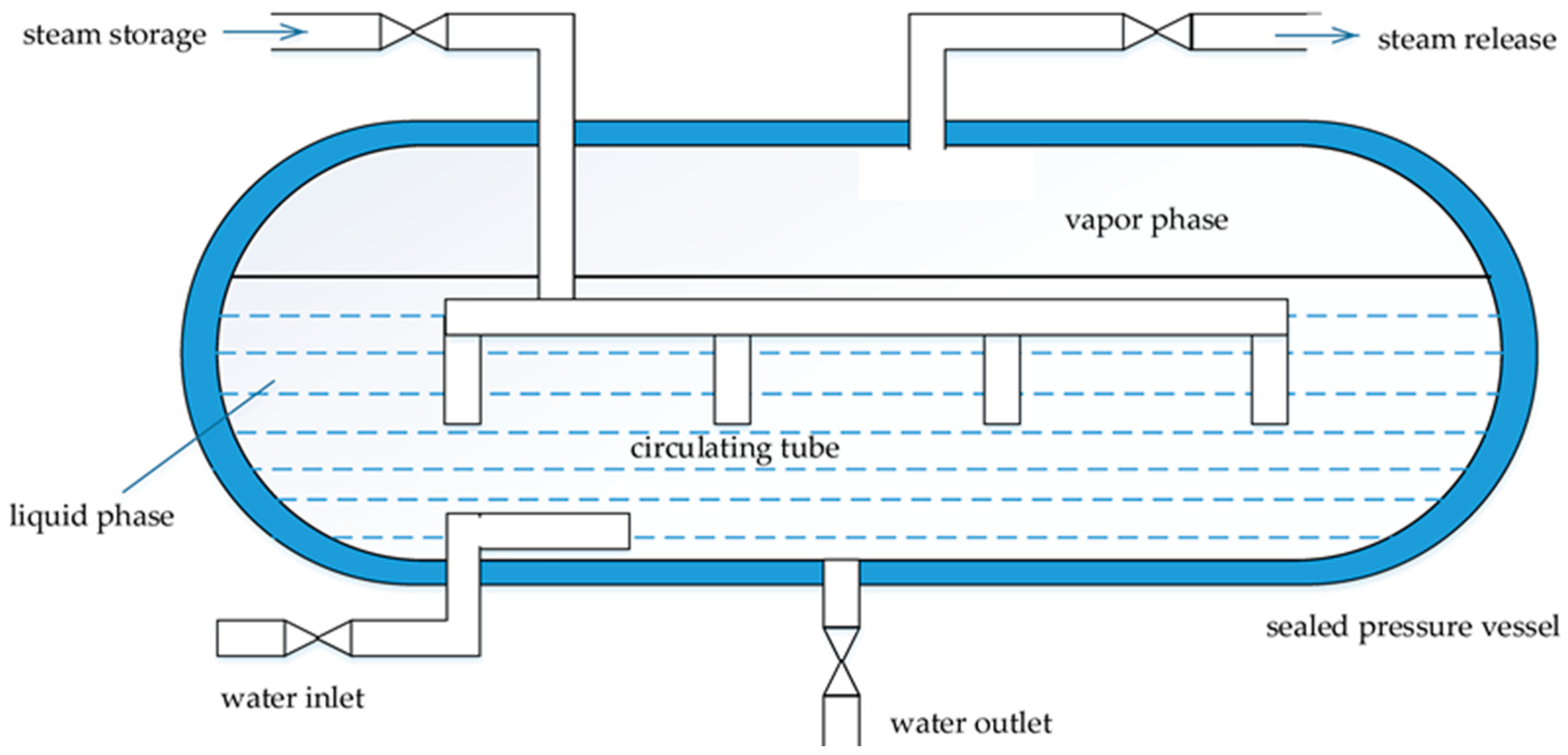
2.1. SA Operation Principle

The operating status of an SA consists of a steam storage process and a steam release process, as shown in Figure 1. The two processes and their operation principles are as follows:
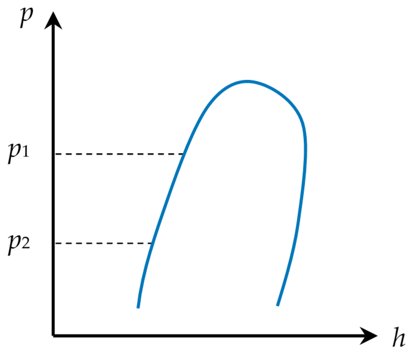
  • Steam storage process: The pressure of steam from a high-temperature SS is higher than that inside the SA. When the steam inlet valve is open, steam flows into the SA automatically. The saturated water and saturated steam with relatively low temperature and pressure is stored in the SA, to which high-temperature steam is added. Through rapid heat exchange, the high-temperature steam is cooled, and the previously mentioned saturated water and steam are heated to a higher temperature to form a new equilibrium state. As the steam storage process continues, it sees a steady rise in the temperature of the water and steam inside the SA, followed by an increasing pressure and water level. Once the internal pressure reaches the specified maximum value, the steam inlet valve closes, and the steam storage process ends. As shown in Figure 2, during the steam storage process, the pressure rises from the specified minimum value p2 to the maximum p1, and the steam is condensed, leading to an increase in the water enthalpy along the saturated liquid line at the left side of Figure 2.
  • Steam release process: This is an inverse process of the steam storage process detailed above. When the SA provides steam for users, the valve at the steam outlet is open. Since the pressure in the steam pipe is lower than that in the SA, the saturated steam in the SA releases automatically under the pressure difference, resulting in a lower pressure inside the SA. When the internal pressure is lower than the saturation pressure corresponding to the temperature of water stored, the saturated water becomes superheated, and the water boils immediately to evaporate as saturated steam. At this point the water temperature and water level in the SA drop until they have decreased to the specified minimum value, at which point the steam outlet valve closes, and the steam release process ends. During this process, the pressure decreases from p1 to p2, as shown in Figure 2, meaning that the superheated water converts to saturated water, and thus, the water enthalpy reduces along the saturated liquid line.

2.2. SS Classification

Usually, SSs are divided into high-, medium-, and low-pressure according to their pressure. In this study, another classification system is used according to the controllability of SS:
  • Controllable steam source (CSS): The steam generation process is of considerable controllability, and therefore, the steam’s flow rate, pressure, and temperature are steady, change periodically, or can be controlled easily, e.g., coal-fired boiler and other station boilers.
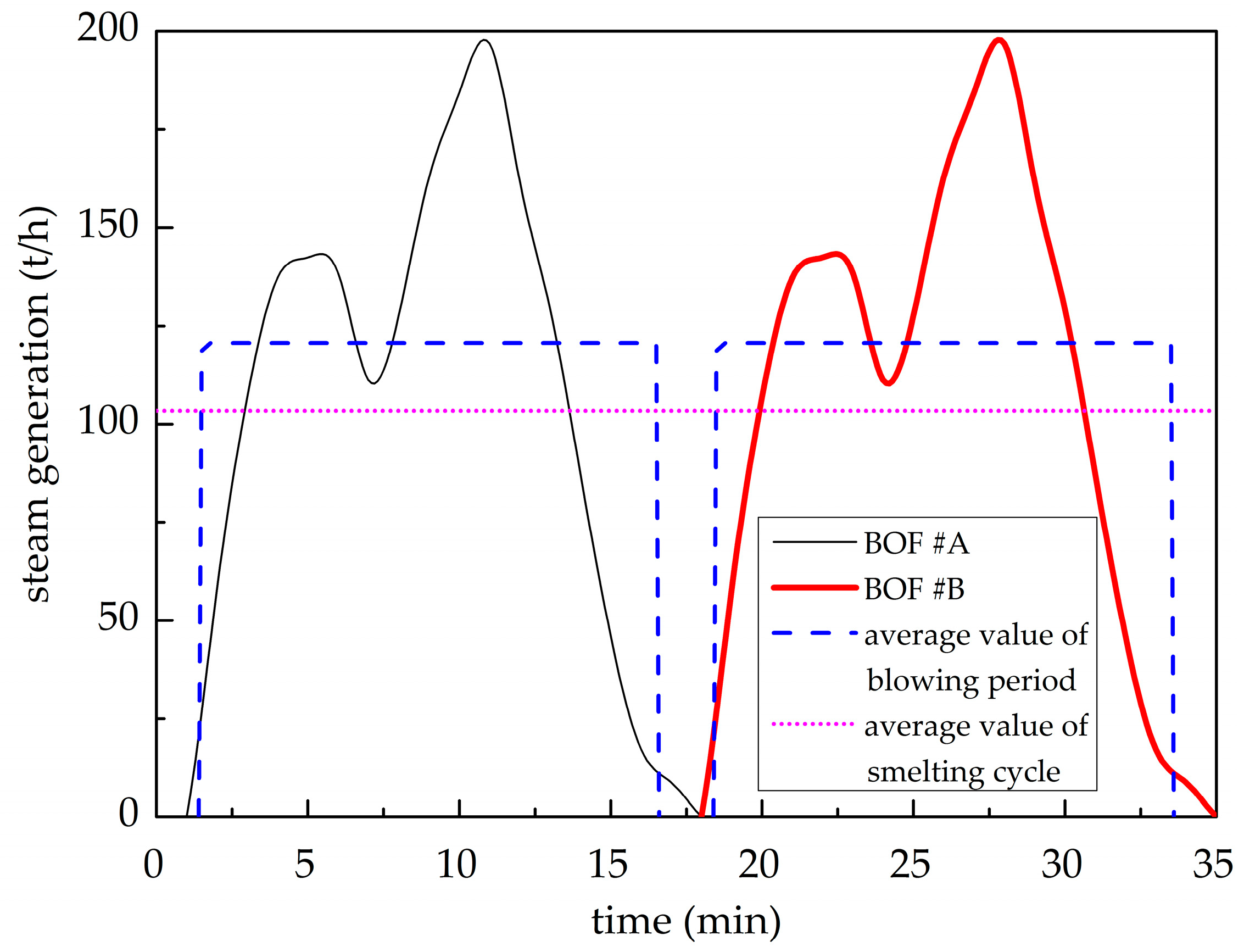
  • Uncontrollable steam source (UCSS): This type generally has the following characteristics: (a) The generation of the steam is influenced by other factors, even randomly intermittent factors; (b) the flow rate of the steam supplied fluctuates frequently; and (c) the temperature and pressure of the steam supplied vary significantly over a large range. It is hard to control the flow rate, pressure, and temperature of steam from UCSSs. Examples include solar thermal plants, incinerators fueled by municipal solid wastes, and basic oxygen furnace (BOF) waste heat power generation.
In both CSSs and UCSSs, SAs are installed between SSs and steam consumers. They can not only exponentially increase the instant steam supply capacity but also stabilize the flow rate, pressure, and temperature of steam supplied at an expected range. Thus, they work both as a thermal energy storage unit and as a buffer unit in the steam supply system, especially for intermittent and fluctuating SSs or steam consumers.

3. Mathematical Model of Steam Accumulator (SA) Operation Optimization

3.1. SA Operation Optimization for UCSS

As mentioned above, the steam generation of UCSSs is easily affected by other random factors, is usually intermittent and frequently fluctuates. Thus, it is of great importance to optimize the operation of SA for UCSSs.
The operating pressure of SAs change within the specified range. The specified maximum value, called charging pressure (p1 in Figure 2), is the highest pressure at the end of the steam storage process. The specified minimum value, called discharging pressure (p2 in Figure 2), is the lowest pressure at the end of steam release process.
The thermal energy storage capacity (TESC) of an SA is the amount of steam mass, or steam thermal energy, generated from the SA from p1 down to p2. For a fixed SA and SS with certain parameters, TESC is determined by the difference between the charging pressure and the discharging pressure. TESC can be increased by increasing the difference between the charging and discharging pressures. For a specified pressure difference, TESC decreases with the increase in discharging pressure. However, the charging pressure cannot be raised freely due to limited pressure of SS and steam pipe resistance. Additionally, discharging pressure is limited by the minimum steam pressure demanded by steam consumers as well as the pipe resistance.
Charging pressure is set as p1, and discharging pressure is set as p2. According to the definition mentioned above,
p 1 = p SS Δ p 1 ,
p 2 = p SC + Δ p 2 ,
where pSS and pSC are the pressures of SS and steam consumers respectively, measured in MPa; ∆p1 is the pressure drop from SS to SA, due to the pipe resistance, measured in MPa; and ∆p2 is the pressure drop from SA to steam consumers, measured in MPa.
The TESCs of the metal part of the SA and vapor phase are neglected because they are much lower than in the water phase in SA. When calculating, only the TESC of the water phase is considered; thus, the volume of an SA can be calculated by:
V = G g × η × φ  
where V is the volume of SA, measured in m3; G is the necessary thermal energy storage capacity (NTESC) of SA, measured in kJ (in caloric) or kg (in mass); η is the SA efficiency and is between 0.98 and 0.99; ϕ is water filling coefficient, which is defined as the ratio of water filling volume to the total SA volume and is approximately 0.9; and g is specific thermal energy storage capacity (STESC), which is defined as the TESC of 1 m3 water from the full storage state to the completely released state, measured in kJ/m3 (in caloric) or kg/m3 (in mass).
The STESC can be determined by two methods: one based on the principle of energy balance, and the other by integrating the steam release equation. In regards to the energy balance method, it is assumed that x kg steam will be generated when 1 kg saturated water changes from p1 to p2, and thus the energy balance equation of steam release process is:
Enthalpy of saturated water (before pressure drop) = Enthalpy of released steam (after pressure drop) + Enthalpy of remaining saturated water (after pressure drop).
In this study, enthalpies are measured by average values. Then,
h 1 = x ( h 1 + h 2 2 ) + ( 1 x ) h 2  
where x is the amount of steam generated per unit water at p2, measured in kg-steam/kg-water; h 1 and h 2 are the enthalpy of saturated water at p1 and p2, respectively, measured in kJ/kg; h 1 and h 2 are the enthalpy of saturated steam at p1 and p2, respectively, measured in kJ/kg.
According to Equation (4), STESC can be expressed as:
g = x × ρ 1 = ρ 1 × h 1 h 2 ( h 1 + h 2 2 ) h 2 ,
where ρ 1 is the density of saturated water at p1, measured in kg/m3.
As for the integral method, it is assumed that X kg water is contained in the SA. The thermal energy of dq (in kJ/kg) will be released when the pressure inside the SA decreases from p to ( p Δ p ) . In addition, the released thermal energy makes dX kg water flash to vapor. The evaporation latent heat of water is r, then
X d q = r d X
thereby
d X X = d q r = d q / T r / T = d s r / T
where d s = d q / T is the entropy change of water, kJ/(kg·K), and T is the absolute temperature of water, K.
Integrating Equation (7) from p1 to p2 yields
ln X 2 X 1 = p 1 p 2 d s r / T
where X1 and X2 are the amount of water at pressure p1 and p2, respectively.
Thus, the STESC can be calculated as
g = X 1 X 2 X 1 × ρ 1 = ρ 1 × ( 1 e p 1 p 2 d s r / T )
According to Equation (9), the STESCs under various charging and discharging pressures are listed in Table 1.
NTESC should be analyzed and calculated based on the real SS condition, the fluctuation regulation of steam consumption load, and the structure of the steam supply system. Initially, it is recommended to work out the average load line according to the real-time steam consumption load curve. Figure 3 is a steam consumption load curve during a cycle. The function of the curve is:
Q = f ( t )
where Q is the real-time steam consumption load, t/h; t is time, in h; f is the function that presents the relationship between Q and t.
The average steam load can be expressed as:
Q ¯ = 1 t 2 t 1 t 1 t 2 f ( t ) d t
where Q ¯ is the average steam consumption load, measured in t/h; t1 and t2 are beginning time and end time, respectively, measured in h.
Then, the difference between real-time load curve and average load line is calculated, and the difference integrated to obtain the integral curve, as shown in Figure 4. The difference between the maximum and minimum points in Figure 4 is the NTESC:
G = Δ Q max Δ Q min  

3.2. SA Operation Optimization for CSS

The steam generation process of a CSS has considerable controllability, and thus, the flow rate, pressure, and temperature of the generated steam can be controlled. It is of great significance to optimize the cooperation of a CSS and an SA. However, SA designers routinely determine the volume of an SA according to steam users without considering its cooperation with a CSS. If it is considered, the operation of an SA and a CSS such as a boiler will be regulated to interact with each other, leading to a minimum SA volume and investment cost.
In a cycle, the steam consumption load is Q(t), and the boiler’s operating load is M(t); thus, the amount of steam that should be stored or released is C ( t ) = M ( t ) Q ( t ) . If C(t) > 0, the SA works in steam storage case, whereas if C(t) < 0, the SA works in steam release case. By integrating C(t), the NTESC can be obtained.
Given that a boiler is generally described by its daily load curve, one day is chosen as a cycle with a time length of 24 h. The number of load records in one hour is R, so the number of total load records is 24R, labelled S = 1, 2, …, 24R. Q(t) can be determined by fitting the 24R load records. The allowed maximum number of changing boiler loads in a cycle is assumed as N, i.e., the allowed maximum segments is N. According to practical experience for a boiler, a load change per 2–3 h has very little influence on its thermal efficiency. The time span between two adjacent load changes is set as L, which is no less than 2 or 3 h.
There are several feasible segmentation schemes satisfying the requirements of N, L, R, and S mentioned above. The optimal segmentation scheme is the one with the lowest NTESC among the feasible schemes. Assume the load record labelled s is the starting time of a cycle. For the k-th segmentation scheme, the beginning time of segment i is bi = ti−1, and the end time is ei = ti. In segment i, the operating load of the boiler at time t is:
M ( t ) = t t i 1 t i t i 1 t i 1 t i Q ( t ) d t .
A set of bi and ei (i = 1, 2, …, N) specifies a segmentation scheme k. If the value of S changes from 1 to 24R, the total number of segments is K:
K = { 1 , ( N = 1 ) 24 R N × R × L + 1 , ( N = 2 ) 1 2 P N 2 = 1 24 R N R L + 1 P N 3 = 1 P N 2 P 2 = 1 P 3 P 1 = 1 P 2 P 1 ( P 1 + 1 ) , ( N 3 )
where P denotes the permissible value of a cut-point in a segment.
For specified L and N, the minimization of NTESC can be expressed as:
{ min G = C max C min ; s . t .   b i = 1 ,   e N = 24 R , L R ( i 1 ) + 1 b i 24 R L R ( N i + 1 ) ,   f o r   i = 2 ,   3 ,   , N , b i + 1 b i L R ,   f o r   i = 1 , 2 , , N 1 , e i = b i + 1 1 ,   f o r   i = 1 , 2 , , N 1 , S = 1 ,   2 , , 24 R , k = 1 , 2 , , K .
To solve the minimization problem (15) to obtain the minimum NTESC and optimal segmentation scheme from all feasible schemes, an optimization algorithm should be developed. The basic process for solving this problem is shown in Figure 5, where a cycle is divided into two segments to be integrated. For each segment, M(t) and C(t) can be calculated by Equation (13) from beginning time bi to end time ei. Starting from scheme A, e1 and b2 is changed gradually and recalculated until scheme B. Then, the starting time of a cycle should change in turn within sets of S, i.e., b1 changes from 1 to 2 to 3, all the way until to 24R; while e2 changes from 24R to 1, to 2, until (24R − 1). The above process is repeated to calculate all feasible two-segment schemes.
When the number of segments reaches N, the exhaustive segmentation schemes can be determined via multiple recursive calls of a basic process. Finally, the optimal scheme, i.e., the minimum NTESC, can be screened out. Note that the beginning time and end time of segment i (see Figure 6) are within the ranges:
{ e i 1 + L R + 1 b i 24 R L R ( N i + 1 ) , b i + L R e i 24 R L R ( N i ) .
The whole process for solving this problem is illustrated in Figure 7.

4. Case Results and Discussion

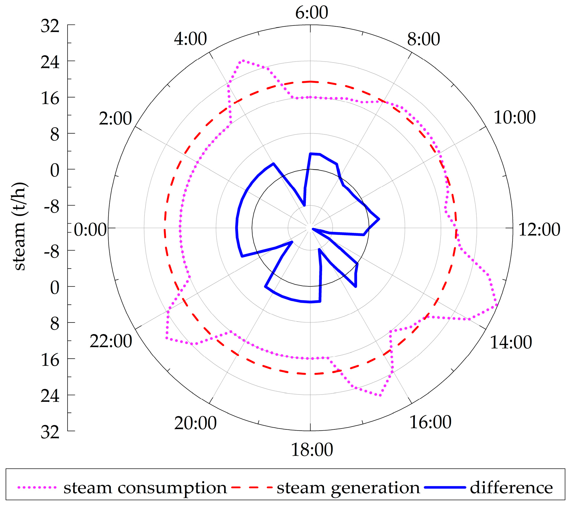
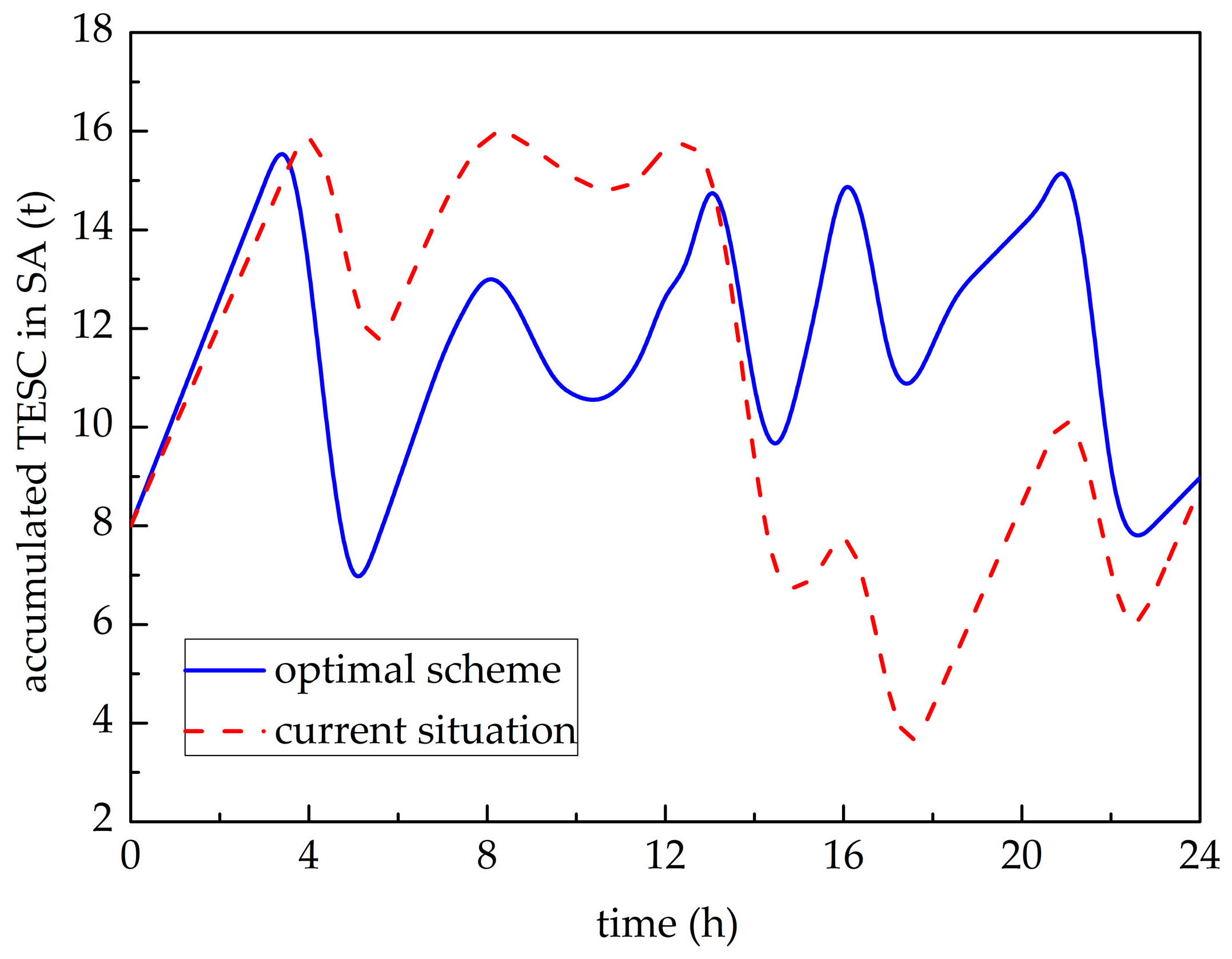
4.1. SA Cooperating with a UCSS

There is a marked steam fluctuation in a BOF waste heat recovery system. The smelting cycle is approximately 30–40 min, of which the oxygen blowing period is approximately 10–16 min. Steam is recovered only during the blowing period. SAs gather the fluctuating and intermittently generated steam and supply that steam to users in a continuous and steady manner.
In a steel-making branch plant of Ansteel, China, there are two BOFs with a nominal capacity of 260 t. Table 2 lists the parameters and Figure 8 shows the steam generation curve of a 260 t BOF. It can be seen from Figure 8 that the oxygen blowing period starts from 9′30″ and ends at 24′30″. From Equation (11), the average steam generation during the oxygen blowing period and the whole smelting cycle can be obtained as follows: the average value of blowing period is 120.64 t/h, and the average value of smelting cycle is 51.70 t/h. The amount of generated steam in one smelting cycle is 30.16 t. Note that there are two peaks. This is because a second oxygen blowing period is usually conducted after the first one, according to the liquid steel detection result of the first blowing period, with the purpose of controlling the carbon content in the liquid steel.
According to the real-time steam generation curve and average steam generation line shown in Figure 8, the NTESC is 17.24 t from Equation (12), as found via integral calculation.
The charging pressure of the SA is the difference between the pressure of steam from the BOF and pipe resistance and has a value of 2.40 MPa. In addition, the discharging pressure is the sum of the pressure of the steam entering the turbines and the pipe resistance and has a value of 1.05 MPa.
The enthalpy of steam can be obtained once the charging pressure and discharging pressure are calculated. From Equation (5) and Table 1, the STESC is 74.6 kg/m3. The water filling coefficient is 0.9, and the thermal efficiency of the SA is 0.99. The volume of the SA for each BOF can be calculated from Equation (3) as 259.30 m3.
With the development of BOF smelting and energy recovery technologies, BOF upgrades towards the large-scale direction, and the amount of steam generated increases. Therefore, it is almost a certainty that the amount of steam needing to be stored or released will rise in the near future. However, the cost of SAs is currently too high to be employed in these cases. An SA cooperating with sets of parallel-operating BOFs may be a more optimized solution that can be economically employed in future steam systems.
To minimize the steam generation peak value, two BOFs blow oxygen in turn, as shown in Figure 9. A smelting cycle is schematically depicted in a rectangle around a dashed line. The starting time is set at 2′30″ later than when BOF #B ends its oxygen blowing. The oxygen blowing period of BOF #A starts from 1′30″ to 16′30″, while BOF #B blows from 18′30″ to 33′30″. Therefore, the case where two BOFs generate steam at the same time can be effectively avoided. The steam generation is shown in Figure 10. The average steam generation during the oxygen blowing period and the whole smelting cycle can be obtained by Equation (11).
It can be seen from Figure 10 that for two parallel-operating BOFs, the average steam generation during oxygen blowing period is 120.64 t/h, and the average value during the whole smelting cycle is 103.40 t/h. According to the real-time steam generation curve and average steam generation line of two parallel-operating BOFs shown in Figure 10, the NTESC is 8.62 t from Equation (12) via integral calculation. The charging pressure and discharging pressure of the SA cooperating with two parallel-operating BOFs are also 2.40 MPa and 1.05 MPa respectively, based on which the enthalpy of steam can be obtained. The STESC is 74.6 kg/m3 from Equation (5). Additionally, the water filling coefficient is 0.9, and the thermal efficiency of the SA is 0.99. Thus, the volume of the SA for the two parallel-operating BOFs is 129.69 m3 according to Equation (3). Compared with the SA cooperating with a single BOF, the volume of SA cooperating with two parallel-operating BOFs is reduced remarkably by 49.98%, with the advantages of less initial investment and less area of land occupied. Note that the optimization results show that two steam sources cooperating with one SA performed even better. It should be noted that use of more than two accumulators in a single system is not discussed in this study.

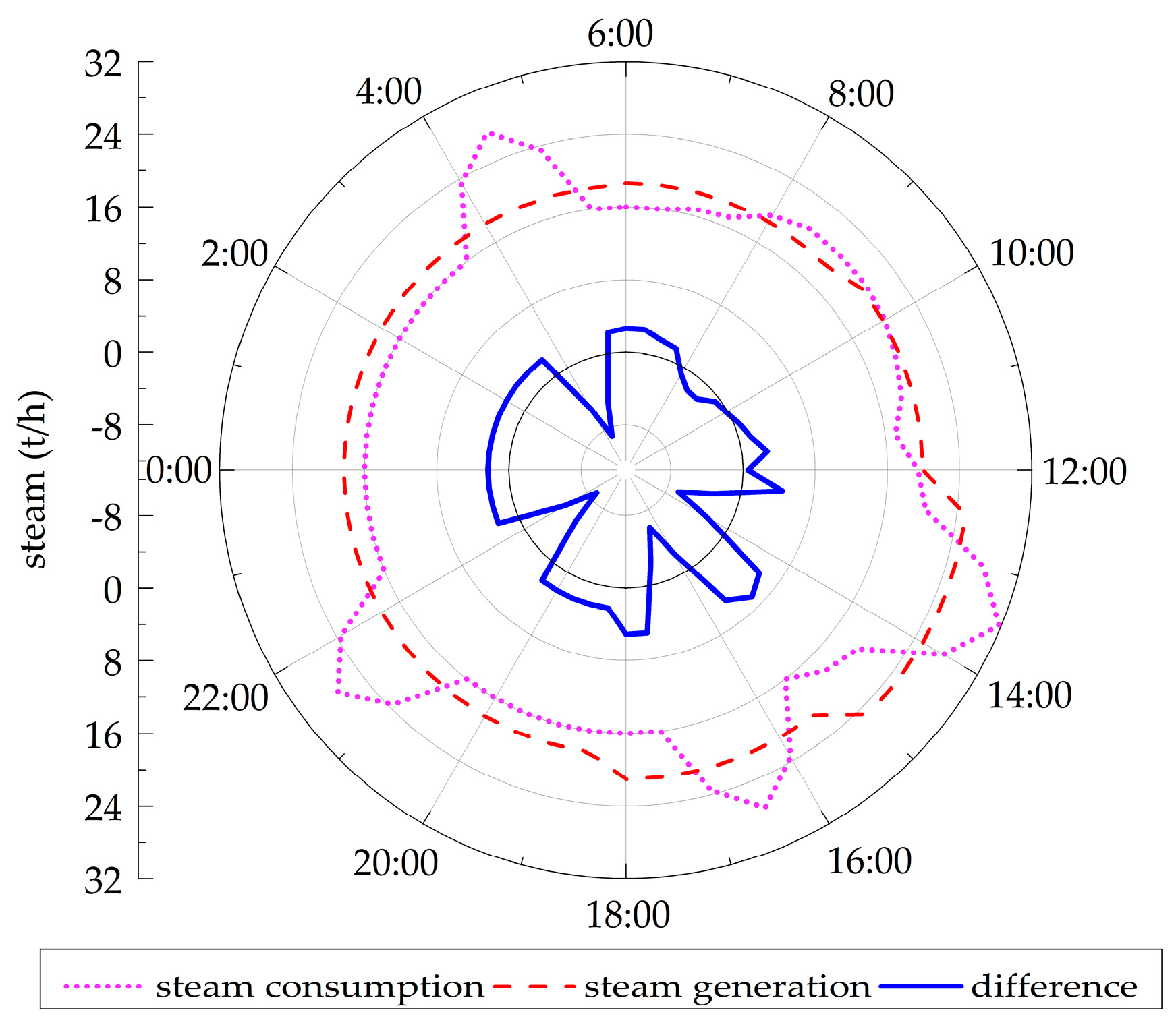
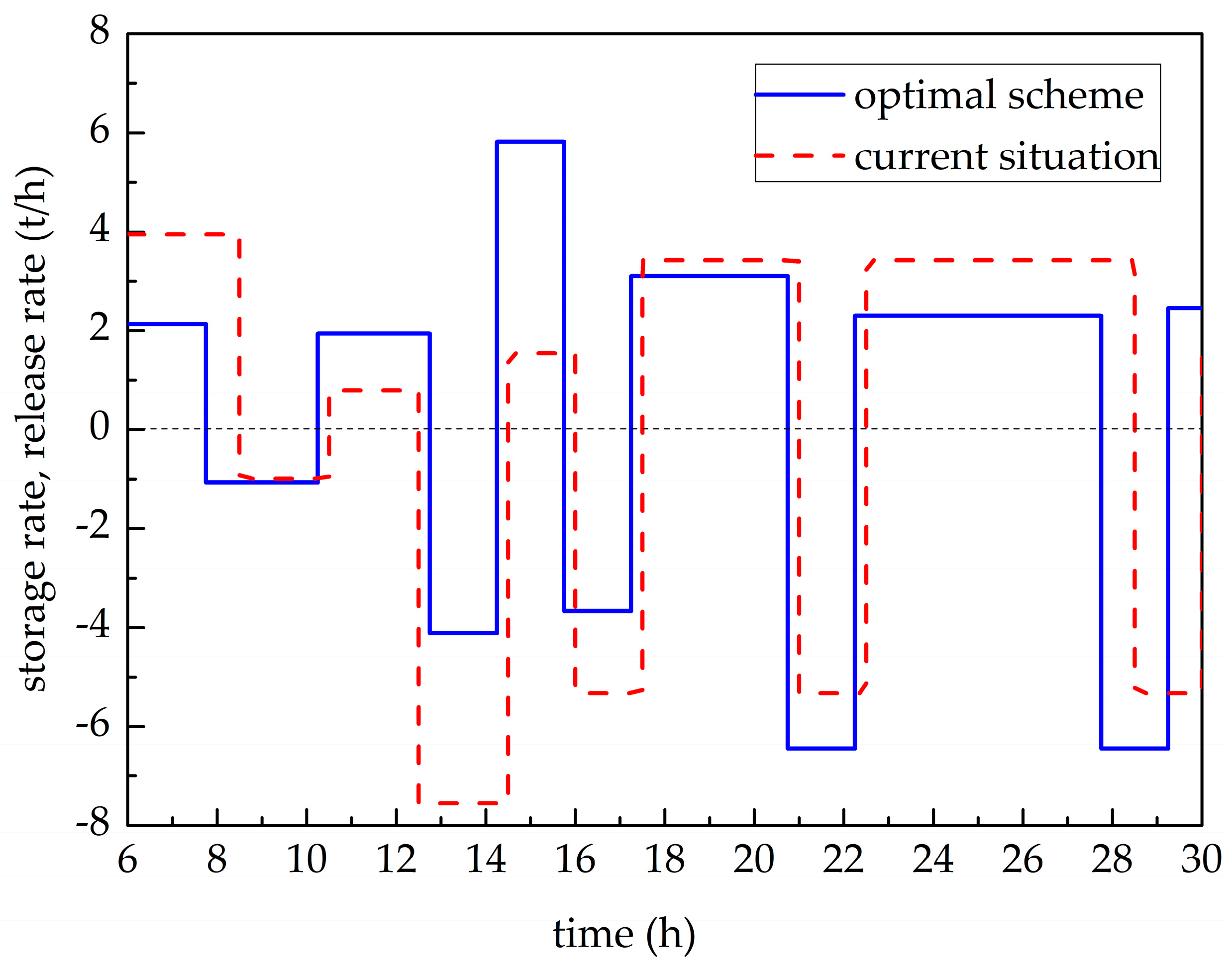
4.2. SA Cooperating with a CSS

Shanghai Heavy Machinery Factory was selected as an example of an SA cooperating with a CSS. In this factory, an SA with the volume of 155 m3 is used in the steam supply system. The relevant parameters are listed in Table 3, and the steam consumption load is shown in Figure 11. It can be seen from Figure 11 that the steam is generated at a constant rate. However, the steam demand of steam consumers varies with time.
The record of steam load in this factory is R = 1. To ensure a relatively high thermal efficiency of the boiler, the time span between two adjacent load changes is set as L ≥ 3. Thus, the number of segments is between 1 and 8. The optimal operation scheme and minimum NTESC can be achieved based on Figure 7. The optimized scheme has five segments: 6:00–9:00, 9:00–12:00, 12:00–15:00, 15:00–18:00, and 18:00–6:00. The steam load curve is presented in Figure 12. Compared with the current operation scheme shown in Figure 11, the steam generation is no longer a constant value throughout the day.
The NTESC of the optimal scheme is 9.064 t from Equation (12). The charging pressure and discharging pressure of the SA are 1.5 MPa and 0.4 MPa, respectively, from which the STESC can be calculated to be 86 kg/m3 via either Equation (5) or Table 1. The water filling coefficient is 0.9, and the thermal efficiency of the SA is 0.99. Thus, according to Equation (3), the volume of the SA is 116 m3. Compared with the current 155 m3 SA, the volume of the optimized operational setup is only 116 m3, which also satisfies the steam consumption load of steam users. The volume reduction rate is 25.16%.
In addition, by comparing Figure 11 and Figure 12, it can be seen that the load difference between steam generation and steam consumption of the optimal setup is between −8.94 t/h and 6.76 t/h, while the current operation is between −12.33 t/h and 3.42 t/h. The maximum load difference of the optimal operation is reduced 27.49% compared to that of the current setup.
The steam is stored in the SA for a cycle time of 8 t. The hourly changes accumulated in the TESC of the optimal operation setup and the current setup are compared in Figure 13. It can be found that the accumulated TESC of the optimized operation setup is smoother than that of the current setup. In the optimal setup, the steam storage and release processes appear in turn, and the levels of transient steam stored and released are equally matched, resulting in a smoother accumulated TESC change. The difference between the maximum and minimum accumulated TESCs in the optimal setup is 9.66 t, rather than 12.91 t in the current setup, with a reduction in fluctuating margin of 25.17%.
Figure 14 compares the steam storage rate and release of the optimal operation setup and the current setup. The variance of the current setup is 797.35, and the variance of the optimal operational setup is 614.24, with an increase of 22.96% in stability. According to [18], there is a tendency towards a non-equilibrium with the increase of steam storage and release rates. Therefore, the optimal operational setup has a more uniform temperature field inside the SA, lower thermal loss and exergy loss, and thus, a better steam storage effect.

5. Conclusions

Steam accumulators (SAs) are used in different applications. Based on the operation principle of an SA and the controllability of steam sources (SSs), SSs are classified in a new way into controllable steam source (CSS) and uncontrollable steam sources (UCSS). When used as a thermal storage unit, thermal energy storage capacity (TESC) is the most important factor that should be considered, while when used as a steam buffer unit, the most important issue is the balance of steam generation and consumption.
For UCSS, the main functions of the SAs are to store emergency steam, to stabilize the fluctuant steam generation, and to make the intermittently supplied steam continuous. The operation of an SA cooperating with a basic oxygen furnace (BOF) as a UCSS has been studied and optimized. It is shown that the optimal operational setup, an SA cooperating with two parallel-operating BOFs, saves 49.98% of the SA volume in the investigated application.
For a CSS, the main function of an SA is to buffer and balance the steam generation and consumption. The mathematical model of the minimum necessary thermal energy storage capacity (NTESC) has been established and solved. Additionally, the optimal operation of an SA in a heavy machinery factory is studied by optimizing the minimum NTESC. The optimized volume of the SA is 116 m3, with a volume reduction rate of 25.16%, a maximum transient load difference reduction of 27.49%, a fluctuating margin reduction of 25.17%, and an increase in steam storage and release stability of 22.96, respectively.

Acknowledgments

This work was supported by the Fundamental Research Funds for the Central Universities, China (N140203002), and the National Natural Science Foundation of China (21561122001).

Author Contributions

Wenqiang Sun designed the overall research; Yuhao Hong developed the mathematical models and retrofitted the configuration; Yanhui Wang analyzed the data; Wenqiang Sun wrote the paper.

Conflicts of Interest

The authors declare no conflict of interest.

Abbreviations

The following abbreviations are used in this manuscript:
BOFbasic oxygen furnace
CSScontrollable steam source
NTESCnecessary thermal energy storage capacity
SAsteam accumulator
SSsteam source
STESCspecific thermal energy storage capacity
TESCthermal energy storage capacity
UCSSuncontrollable steam source

References

  1. Castro-Dominguez, B.; Mardilovich, I.P.; Ma, L.C.; Ma, R.; Dixon, A.G.; Kazantzis, N.K.; Ma, Y.H. Integration of methane steam reforming and water gas shift reaction in a Pd/Au/Pd-based catalytic membrane reactor for process intensification. Membranes 2016, 6, 44. [Google Scholar] [CrossRef] [PubMed]
  2. Kessy, H.N.E.; Hu, Z.; Zhao, L.; Zhou, M. Effect of steam blanching and drying on phenolic compounds of litchi pericarp. Molecules 2016, 21, 729. [Google Scholar] [CrossRef] [PubMed]
  3. Shamsi, S.; Omidkhah, M.R. Optimization of steam pressure levels in a total site using a thermoeconomic method. Energies 2012, 5, 702–717. [Google Scholar] [CrossRef]
  4. Sun, W.; Zhao, Y.; Wang, Y. Electro- or turbo-driven?—Analysis of different blast processes of blast furnace. Processes 2016, 4, 28. [Google Scholar] [CrossRef]
  5. Ma, G.; Cai, J.; Zhang, L.; Sun, W. Influence of steam recovery and consumption on energy consumption per ton of steel. Energy Procedia 2012, 14, 566–571. [Google Scholar] [CrossRef]
  6. Yu, J. Status and transformation measures of industrial coal-fired boiler in China. Clean Coal Technol. 2012, 18, 89–91. (In Chinese) [Google Scholar]
  7. Tanton, D.M.; Cohen, R.R.; Probert, S.D. Improving the effectiveness of a domestic central-heating boiler by the use of heat storage. Appl. Energy 1987, 27, 53–82. [Google Scholar] [CrossRef]
  8. Elman, J.L. Finding structure in time. Cogn. Sci. 1990, 14, 179–211. [Google Scholar] [CrossRef]
  9. Sabihuddin, S.; Kiprakis, A.E.; Mueller, M. A numerical and graphical review of energy storage technologies. Energies 2015, 8, 172–216. [Google Scholar] [CrossRef]
  10. Shnaider, D.A.; Divnich, P.N.; Vakhromeev, I.E. Modeling the dynamic mode of steam accumulator. Auto Remote Control 2010, 71, 1994–1998. [Google Scholar] [CrossRef]
  11. Bai, F.; Xu, C. Performance analysis of a two-stage thermal energy storage system using concrete and steam accumulator. Appl. Therm. Eng. 2011, 31, 2764–2771. [Google Scholar] [CrossRef]
  12. Xu, E.; Yu, Q.; Wang, Z.; Yang, C. Modeling and simulation of 1 MW DAHAN solar thermal power tower plant. Renew. Energy 2011, 36, 848–857. [Google Scholar] [CrossRef]
  13. Chen, G.Q.; Yang, Q.; Zhao, Y.H.; Wang, Z.F. Nonrenewable energy cost and greenhouse emissions of a 1.5 MW solar power tower plant in China. Renew. Sustain. Energy Rev. 2011, 15, 1961–1967. [Google Scholar] [CrossRef]
  14. Price, N. Steam accumulators provide uniform loads on boilers. Chem. Eng. 1982, 89, 131–135. [Google Scholar]
  15. Studovic, M.; Stevanovic, V. Non-equilibrium approach to the analysis of steam accumulator operation. Thermophys. Aeromech. 1994, 1, 53–60. [Google Scholar]
  16. Stevanovic, V.D.; Maslovaric, B.; Prica, S. Dynamics of steam accumulation. Appl. Therm. Eng. 2012, 37, 73–79. [Google Scholar] [CrossRef]
  17. Stevanovic, V.D.; Petrovic, M.M.; Milivojevic, S.; Maslovaric, B. Prediction and control of steam accumulation. Heat Transf. Eng. 2015, 36, 498–510. [Google Scholar] [CrossRef]
  18. Maklakov, N.N.; Khramov, S.M. Application of a heat hydraulic accumulator to thermal stabilization of the evaporation zone of a heat pipe. J. Eng. Phys. Thermophys. 2003, 76, 1–5. [Google Scholar] [CrossRef]
  19. Walter, H.; Linzer, W. Flow stability of heat recovery steam generators. J. Eng. Gas Turbines Power 2006, 128, 840–848. [Google Scholar] [CrossRef]
  20. Liu, X.; Gong, C.; Liu, S.; Nie, Q. Analytical calculation and experimental study on temperature rising process of steam accumulator. Acta Energiae Solaris Sin. 1998, 19, 102–104. [Google Scholar]
  21. Yang, S.; Manning, B.W. Fitness for service evaluation of cracked divider plate bolt locking tabs for nuclear steam generators. Nucl. Eng. Des. 2009, 239, 2242–2264. [Google Scholar] [CrossRef]
  22. Steinmann, W.D.; Eck, M. Buffer storage for direct steam generation. Sol. Energy 2006, 80, 1277–1282. [Google Scholar] [CrossRef]
  23. Su, S.; Huang, S.Y.; Wang, X.M. Experiments and homogeneous turbulence model of boiling flow in narrow channels. Heat Mass Transf. 2005, 41, 773–779. [Google Scholar]
  24. Engelhardt, G.R.; Macdonald, D.D.; Millett, P.J. Transport processes in steam generator crevices. II. A simplified method for estimating impurity accumulation rates. Corros. Sci. 1999, 41, 2191–2211. [Google Scholar] [CrossRef]
  25. Cao, J. Optimization of thermal storage based on load graph of thermal energy system. Int. J. Thermodyn. 2000, 3, 91–97. [Google Scholar]
  26. Valenzuela, L.; Zarza, E.; Berenguel, M.; Camacho, E.F. Direct steam generation in solar boilers. IEEE Control Syst. Mag. 2004, 24, 15–29. [Google Scholar] [CrossRef]
Figure 1. Schematic layout of a steam accumulator (SA).
Energies 10 00017 g001
Figure 2. Pressure-enthalpy diagram of steam storage and release processes. Pressure varies within p1 to p2 in the whole SA operating process.
Energies 10 00017 g002
Figure 3. Steam consumption load curve during a cycle. The curve denotes the real-time load; the straight line denotes the average load; the shadow in horizontal line denotes the steam storage; and the shadow in vertical line denotes the steam release.
Energies 10 00017 g003
Figure 4. Integral curve of load difference. It is the integral of the difference between real-time load and average load. G is the difference between the maximum and minimum values on the integral curve.
Energies 10 00017 g004
Figure 5. Basic process of model solving.
Energies 10 00017 g005
Figure 6. Recursive call of basic process for segment number at N.
Energies 10 00017 g006
Figure 7. Problem solving flow chart. NTESC: necessary thermal energy storage capacity.
Energies 10 00017 g007
Figure 8. Steam generation of a 260 t BOF. The solid line denotes the real-time load value; the dashed line denotes the average value of the blowing period; and the short dot denotes the average value of smelting cycle.
Energies 10 00017 g008
Figure 9. Schematic diagram of alternated operation of BOFs. The shadowed zones denote the oxygen blowing periods. The dashed rectangle denotes a melting cycle.
Energies 10 00017 g009
Figure 10. Steam generation of two 260 t parallel-operating BOFs. The fine line denotes the real-time load of BOF #A; the heavy line denotes the real-time load of BOF #B; the dashed line denotes the average value of the two BOFs of blowing period; and the short dot denotes the average value of the two BOFs of smelting cycle.
Energies 10 00017 g010
Figure 11. Daily steam consumption load curve. The dashed line denotes the steam generation; the short dot denotes the steam consumption; and the solid line denotes the difference between steam generation and steam consumption.
Energies 10 00017 g011
Figure 12. Load diagram of the optimal operation scheme. The dashed line denotes the steam generation; the short dot denotes the steam consumption; and the solid line denotes the difference between steam generation and steam consumption.
Energies 10 00017 g012
Figure 13. Comparison of accumulated thermal energy storage capacity (TESC) of the optimal and current operational setups. The dashed line denotes the current setup; and the solid line denotes the optimal setup.
Energies 10 00017 g013
Figure 14. Comparison of steam storage rate and release rate of the two setups. The dashed line denotes the current setup; and the solid line denotes the optimal setup.
Energies 10 00017 g014
Table 1. Specific thermal energy storage capacities (STESCs) under different charging and discharging pressures (in kg/m3).
Disharing Pressure (MPa)Charging Pressure (MPa)
0.70.80.91.01.21.41.51.61.82.02.22.4
0.26674818799110115119127136143149
0.348576571849599104113121127134
0.43342505769818691100108116122
0.522313946597076809097106112
0.6--283447596569788795102
0.7----3850566170788692
0.8------475363717884
0.9-------4455637076
1.0--------47566470
1.1---------495763
1.2---------435056
Table 2. Parameters of basic oxygen furnaces (BOFs), steam accumulators (SAs), and generated steam.
ItemValueUnit
nominal capacity of BOF260t
smelting cycle of BOF35min
oxygen blowing period of BOF15min
pressure of generated steam2.45MPa
temperature of generated steam223°C
charging pressure of SA2.40MPa
discharging pressure of SA1.05MPa
water filling coefficient of SA0.90-
thermal efficiency of SA0.99-
Table 3. Parameters of SA.
ItemValueUnit
charging pressure of SA1.50MPa
discharging pressure of SA0.40MPa
water filling coefficient of SA0.90-
thermal efficiency of SA0.99-

