Performance Analysis of Data-Driven and Model-Based Control Strategies Applied to a Thermal Unit Model

Abstract

The paper presents the design and the implementation of different advanced control strategies that are applied to a nonlinear model of a thermal unit. A data-driven grey-box identification approach provided the physically–meaningful nonlinear continuous-time model, which represents the benchmark exploited in this work. The control problem of this thermal unit is important, since it constitutes the key element of passive air conditioning systems. The advanced control schemes analysed in this paper are used to regulate the outflow air temperature of the thermal unit by exploiting the inflow air speed, whilst the inflow air temperature is considered as an external disturbance. The reliability and robustness issues of the suggested control methodologies are verified with a Monte Carlo (MC) analysis for simulating modelling uncertainty, disturbance and measurement errors. The achieved results serve to demonstrate the effectiveness and the viable application of the suggested control solutions to air conditioning systems. The benchmark model represents one of the key issues of this study, which is exploited for benchmarking different model-based and data-driven advanced control methodologies through extensive simulations. Moreover, this work highlights the main features of the proposed control schemes, while providing practitioners and heating, ventilating and air conditioning engineers with tools to design robust control strategies for air conditioning systems.

1. Introduction

The energy cost used in buildings for the developed countries in Europe was very high, up to 50% of which was due to air conditioning systems. On the other hand, water heating represented 13%, whilst lighting and electric appliances contributed to a further 12% in 2015 [1,2]. Air conditioning modules in buildings yield to heating/cooling tools, which can require also the regulation of advanced thermal comfort parameters represented by the air relative humidity and its temperature. The thermal unit (TU) module is fundamental in these systems, as it supplies the properly-treated air to the buildings. Therefore, the dynamic behaviour of TU modules represents the key point for decreasing the energy consumption and achieving the thermal comfort in buildings [3].

The TU module can be described as a nonlinear time-invariant multivariable dynamic process, which is affected by disturbance and uncertainty terms when analysed for control applications [4,5]. Different control schemes exploited classic regulation approaches, such as on-off control laws and proportional, integral and differential (PID) standard compensators [6,7,8]. These control schemes are simple with low-cost implementations, but sometimes unable to achieve accurate solutions. Moreover, the TU module can include nonlinear functions [9], such as products between air temperature and mass flow rate, which can require advanced control strategies to achieve more complex thermal comfort indices and lower energy consumption. To overcome these problems, control strategies relying on artificial intelligence (AI) tools, namely artificial neural networks (ANN), fuzzy logic (FL), adaptive neuro-fuzzy inference systems (ANFIS) and model predictive controllers (MPC) have been proposed to obtain more advanced comfort issues in building applications [10,11,12,13]. As an example, an FL control scheme was proposed in [14], where the heat, the humidity and the oxygen particle concentration represented the control variables, while the fresh air inflow and the fan circulation rate were the monitored outputs. It was shown that FL allowed for more accurate and straightforward results when compared to linear control schemes. A different FL controller to regulate the air conditioning system temperature was proposed in [15], which was able to easily manage the system nonlinearity.

Other contributions considered different ANN tools that are able to enhance the design of suitable controllers used in air conditioning applications [3,12]. As an example, ANN controllers were proposed in [12] for an air conditioning system and compared with a standard PID regulator. It was shown how these ANN controllers allowed one to achieve a controlled output with a shorter settling time and almost zero overshoot. The main advantage of ANN controllers is represented by their interesting features of automatic learning, easy adaptation and straightforward generalisation. However, more efficient solutions were proposed and based on the ANFIS tool [15,16,17,18]. In particular, in [15], ANFIS was successfully exploited as an alternative control strategy with heating, ventilation and air conditioning (HVAC) systems to achieve accurate tracking errors.

Other works proposed MPC schemes for the temperature control of buildings [2,19,20,21]. As an example, in [2], it was shown that the MPC scheme was able to achieve both thermal comfort and energy saving features. Similarly, [19] suggested a more efficient control method when compared with traditional weather-compensated control schemes. Moreover, [22] addressed an interesting overview of MPC methodologies for HVAC systems.

Note that recent studies considered the achievement of thermal comfort and energy efficiency issues using AI tools. However, the performances obtained by these AI-based methods were not analysed in detail and compared via extensive simulations as proposed in this paper using the Monte Carlo (MC) tool. Moreover, this work illustrates the design and the implementation of different control schemes with application to a nonlinear TU dynamic module proposed by the same authors in [9]. Note also that the same authors presented some preliminary results in [23,24,25], but the analysis of the achievable properties and the robustness features of the proposed solutions with their reliability characteristics have been described in detail in this paper.

Another key issue of the present study consists of illustrating the viable application of the suggested control schemes to real air conditioning systems. This point is fundamental for enhancing practitioners and HVAC young engineers to acquire the fundamentals and the basic design tools for effective HVAC controller development and application. To this aim, the suggested simulations have been synthesised in the MATLAB^® and Simulink^® environments and exploiting their standard toolboxes or free software tools. Note that some control strategies proposed in this work were already successfully applied to nonlinear models of energy conversion systems as shown, e.g., in [26,27,28].

Finally, it is worth observing that several research papers have already dealt with this issue in the past (see, e.g., [22,29]), even if they are limited to MPC solutions. However, this work recalls, analyses and implement different control solutions when applied to the thermal unit model already developed by the authors in [9]. Therefore, the key contribution of the work consists of investigating the viability and the reliability features of the proposed solutions with respect to the considered application example. The control performances achieved in simulation are verified and validated by means of the Monte Carlo tool. The proposed control strategies and the validation tools serve to highlight the potential application of the suggested methodologies to real dynamic processes, such as passive and active air conditioning systems.

The remainder of the paper is organised as follows. Section 2 provides an overview of the TU module and its mathematical description. Section 3 illustrates the suggested control schemes exploited in this study, whilst the obtained results are reported in Section 4. The reliability and robustness characteristics of the proposed tools in simulation are discussed in Section 4.1. Finally, Section 5 ends the work by summarising the main achievements of the paper. Open problems and future issues that require further investigations are also suggested.

2. Thermal Unit Mathematical Description

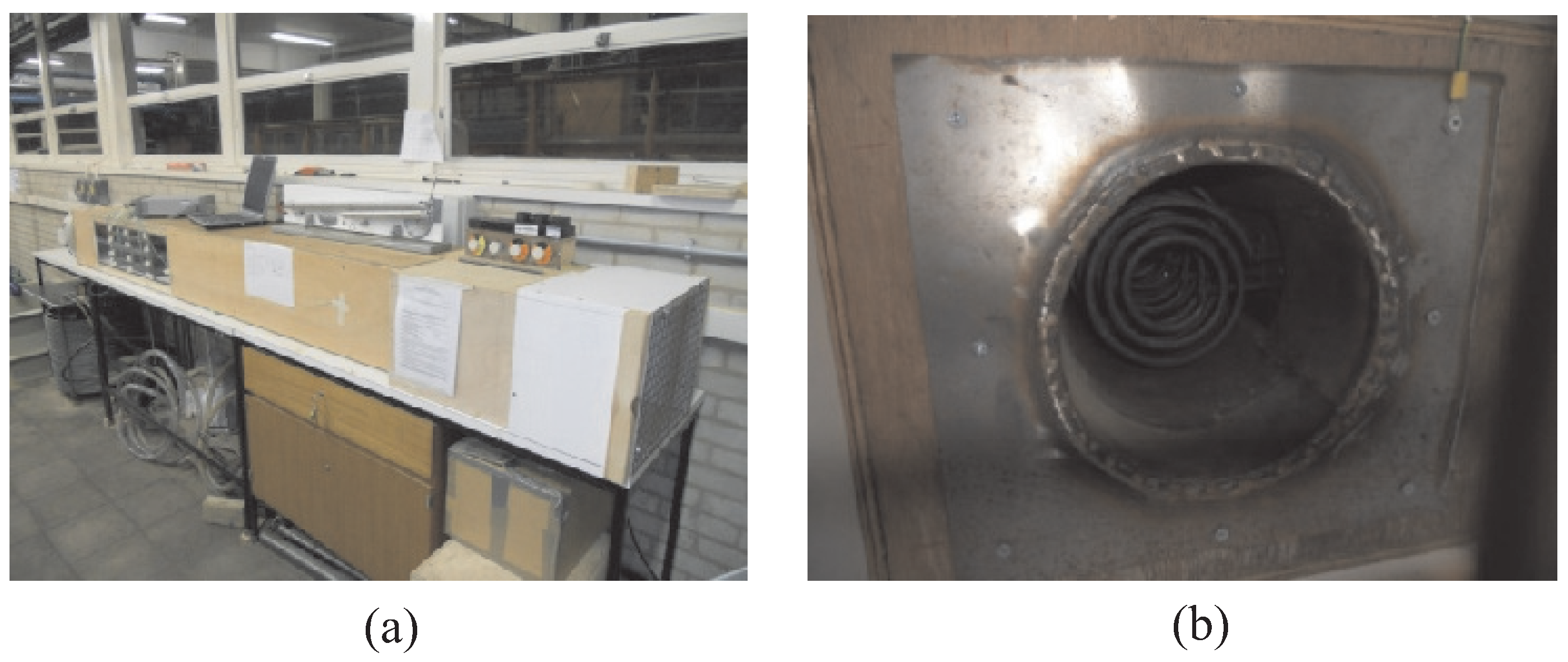
The TU module considered in this study consists of a fundamental block of the whole test-rig proposed for the description and the assessment of the dynamic behaviour of phase change material (PCM) systems used in passive air conditioning plants. Figure 1 represents the complete PCM system facility considered in [9], where the air flow speed and the temperature are the controlled variables that are exploited to perform the presented simulations and experiments. The heating element included into the PCM system is also sketched.

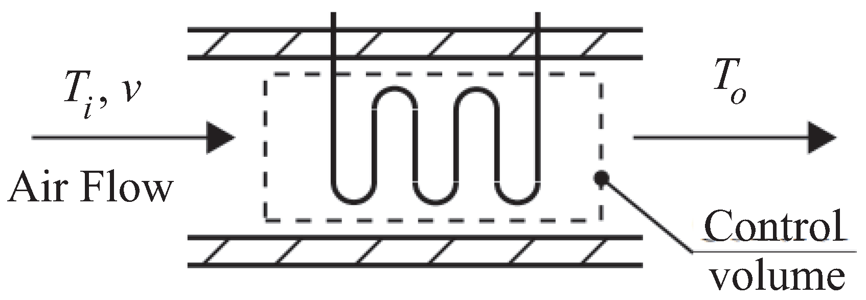
On the other hand, Figure 2 illustrates how the inflow air is treated by means of the heating element (HE) of the TU. Moreover, the TU module is in a downstream series connection with a cooling unit, which is not reported in Figure 2.

With reference to Figure 2, the measured inlet air temperature, $T_i$ (K), and the air velocity, v (m/s), represent the system inputs considered in this study for describing the dynamic behaviour of the TU module. On the other hand, the system output is the outlet air temperature, $T_o$ (K). The experimental data are acquired from the test-rig of Figure 1, such that the HE sketched in Figure 2 supplies a constant power q (W), with an average value of $q=830$ (W). As highlighted in Figure 2, the signal measurements of v, $T_i$ and $T_o$ are acquired from the cross-sectional area centre of the supply duct. Note that the input $T_i\left(t\right)$ is considered as a disturbance acting on the controlled system.

The mathematical expressions describing the energy balance of the TU module, its air control volume and the energy balance with respect to the adjacent duct walls have the following form:

$$\begin{array}{}\mathrm{(1)}& \hfill C_h\frac{d{T}_h\left(t\right)}{dt}& =& q\left(t\right)-{\left(UA\right)}_h\left(T_h\left(t\right)-T_o\left(t\right)\right)\hfill \mathrm{(2)}& \hfill 0& =& {\left(UA\right)}_h\left(T_h\left(t\right)-T_o\left(t\right)\right)-v\left(t\right){\rho }_a{A}_a{c}_a\left(T_o\left(t\right)-T_i\left(t\right)\right)-{\left(UA\right)}_{\mathrm{int}}\left(T_o\left(t\right)-T_w\left(t\right)\right)\hfill \mathrm{(3)}& \hfill C_w\frac{d{T}_w\left(t\right)}{dt}& =& {\left(UA\right)}_{\mathrm{int}}\left(T_o\left(t\right)-T_w\left(t\right)\right)-{\left(UA\right)}_{\mathrm{ext}}\left(T_w\left(t\right)-T_a\left(t\right)\right)\hfill \end{array}$$

where the variable $C_h$ (J/K) indicates the heating element thermal capacity, $C_w$ (J/K) is the thermal wall capacity (insulated plywood), $c_a$ (J/kg·K) represents the air specific heat capacity, $A_a$ (m²) is the cross-sectional area of the duct, ${\rho }_a$ (kg/m³) denotes the air density, $q\left(t\right)$ represents the supplied constant heat gain, whilst U (J/m²·K) indicates the heat transfer coefficient. Note that in Equations (1)–(3), the term ${\left(UA\right)}_h$ (J/K) indicates the product of the heat transfer coefficient U (J/m²·K) with the efficient surface area, A (m²), through which the heat is transmitted and regarding the TU module. On the other hand, ${\left(UA\right)}_{\mathrm{int}}$ (J/K) indicates the coefficient with reference to the inner duct wall, whilst ${\left(UA\right)}_{\mathrm{ext}}$ (J/K) denotes the same term regarding the outer duct wall.

The variables $T_h\left(t\right)$ (K), $T_w\left(t\right)$ (K) and $T_a\left(t\right)$ (K) denote the average heating element temperature, the wall temperature and outside air temperature, respectively. Note that the air surrounding the heating element is assumed to be perfectly mixed. Therefore, the outlet air temperature $T_o\left(t\right)$ is equal to the mean temperature of the whole control volume under the lumped parameter modelling approach (see Equation (1)). Moreover, the thermal capacity of the air passing thought the TU element of Figure 2 is assumed to be very small, so that the heat transfer between the heating element and the air is instantaneous. Under this assumption, the left side of Equation (2) is zero. Finally, in Equation (3), it is assumed that the heat loss occurs only through the walls of the duct.

A standard thermocouple type K has been used to measure the air temperatures. The accuracy is around 1 ^∘C for the whole measurement range. The airflow has been measured using a Hot Wire Thermo-Anemometer with a declared accuracy of $5\%$. For more details regarding the TU module, which is beyond the scope of this paper, the interested reader is referred to [9].

The authors in [9] showed that the complete dynamic behaviour of the TU module is described by a continuous-time time-invariant nonlinear model consisting of a product of two second-order continuous-time time-invariant transfer functions in the form of Equation (4):

$$T_o\left(t\right)=\frac{{\widehat{\beta }}_{1}s+{\widehat{\beta }}_2}{s^2+{\widehat{\alpha }}_{1}s+{\widehat{\alpha }}_2}\left(T_i\left(t\right)v\left(t\right)\right)+\frac{{\widehat{\eta }}_{1}s+{\widehat{\eta }}_2}{s^2+{\widehat{\alpha }}_{1}s+{\widehat{\alpha }}_2}\left(T_o\left(t\right)v\left(t\right)\right)+\widehat{\epsilon }$$

(4)

where s denotes a differential operator. The parameters ${\widehat{\alpha }}_i$, ${\widehat{\beta }}_i$, ${\widehat{\eta }}_i$ and $\widehat{\epsilon }$ of the model in the form of Equation (4) were obtained by using a refined instrumental variable method described in [9]. These values are reported in

Table 1. Estimated model parameters with their accuracy [9].

Parameter	${\widehat{\mathit{\alpha }}}_1$	${\widehat{\mathit{\alpha }}}_2$	${\widehat{\mathit{\beta }}}_1$	${\widehat{\mathit{\beta }}}_2$
Value	55.026 ± 2.011	−92.835 ± 3.398	9.9837 ± 0.2512	7.7661 ± 0.2835
Parameter	${\widehat{\mathit{\eta }}}_{\mathbf{1}}$	${\widehat{\mathit{\eta }}}_{\mathbf{2}}$	$\widehat{\mathit{\epsilon }}$
Value	−8.5689 ± 0.2070	−8.3067 ± 0.2984	−122.95 ± 4.426

.

The model is considered to be of low complexity yet achieves high simulation performance. The physical meaningfulness of the model provides enhanced insight into the performance and functionality of the system. In return, this information can be used during the system simulation and improved model-based and data-driven control designs for temperature regulation, as shown in the following sections.

3. Control Designs for the TU Module

With reference to the systems sketched in Figure 2 and modelled by the expressions of Equations (1)–(3), the general plant can be described as a Multiple-Input Single-Output (MISO) time-invariant nonlinear model, where the input-output air temperatures and its air flow represent the main input-output variables. Its input-output dynamic behaviour can be described as a nonlinear dynamic function $\mathcal{F}$ in the general form of Equation (5):

$$y\left(t\right)=\mathcal{F}\left(u\left(t\right),t\right)$$

(5)

where $y\left(t\right)$ is the output variable, i.e., $T_o\left(t\right)$, $u\left(t\right)$ is the input vector, i.e., ${\left[T_i\left(t\right),v\left(t\right)\right]}^T$ and t is the time. The control law designed to be applied to the TU module in general determines the control input injected into the controlled plant of Equation (5) in order to track a given reference, or set-point, denoted as $r\left(t\right)$.

It is worth observing that the design and the performance of control systems for generic TU processes are strongly determined by the bilinear terms represented in Equation (4), where the nonlinear behaviour is described by the product between the air temperature and its mass flow rate. Under this consideration, in order to enhance the control law designs and their implementation, the inlet air temperature $T_i\left(t\right)$ is considered as a measurable disturbance $d\left(t\right)$. The input-output data acquired from the test-rig and the TU module in Figure 1 and Figure 2 are represented by the inlet air temperature $T_i\left(t\right)$, the air flow $v\left(t\right)$ and the outlet air temperature $T_o\left(t\right)$.

In the remainder of this section, different control laws and their implementations are summarised. The methods include the standard PID regulator and nonlinear control methodologies relying on AI techniques, such as FL and adaptive schemes, as well as the model predictive control. These control strategies, which are exploited for the the regulation of the outlet air temperature $T_o\left(t\right)$, will be applied to the TU system of Figure 2 described by the model of Equation (4).

3.1. Standard PID Controller Design

Several works [5,6,7,12,30] highlighted that standard PID controllers can be commonly used in general HVAC applications. In fact, it is shown that simple PID controllers are able to achieved interesting results based on the direct and straightforward computation of the tracking error $e\left(t\right)$ computed as the difference between the reference and the measured values of the output, respectively, i.e., $e\left(t\right)=r\left(t\right)-y\left(t\right)$. The continuous-time standard PID controller can be represented in the following parallel form [31,32]:

$$u\left(t\right)=K_p+K_i{\int }_0^{t}e\left(\tau \right)d\tau +K_d\frac{de\left(t\right)}{dt}$$

(6)

where $Kp$, $K_i$ and $K_d$ are the PID proportional, integral and derivative gains, respectively. Note that the derivative term of the PID controller is usually implemented as the first-order filter whose pole location is defined by the time–constant $T_f$. The derivation of the PID gains when this standard controller is applied to the TU module of Section 2 will be achieved by means of the auto-tuning approach proposed, e.g., in [32] and implemented in the MATLAB^® environment.

3.2. Fuzzy Controller Design

A controller relying on the FL strategy can be described as statements $IF$–$THEN$–$ELSE$, as addressed, e.g., in [33,34]. Successful application of FL to HVAC systems was presented, e.g., in [35,36]. This work will show that the derivation of the controller mathematical description can exploit the direct identification of rules in the form of Takagi–Sugeno (TS) prototypes [37]. These models can be derived by exploiting the ANFIS tool already available from the Simulink^® toolbox [38].

According to this description, the TS fuzzy prototype relies on a suitable number of rules denoted as $R_i$, where the consequent terms are deterministic functions in the form of $f_i(.)$. The subscript i indicates the i-th rule, which is usually represented in the form of:

$$R_i:IFx\in A_{i}THEN{y}_i=f_i\left(x\right)$$

(7)

where $i=1,2,\dots ,K$ and K represents a suitable number of rules. In Equation (7), the variable x indicates the antecedent terms, whilst the scalar $y_i$ represents the consequent output. For the i-th rule, the fuzzy set $A_i$ is represented in general by a multivariable membership function ${\mu }_{A_i}(.)$ described by the relation of Equation (8) [39]:

$${\mu }_{A_i}\left(x\right):A_i\left(x\right)\mapsto [0,1]$$

(8)

The consequent functions $f_i(.)$ can be represented by parametric models, with fixed structure and varying parameters, as addressed by the same authors, e.g., in [40]. The function $f_i(.)$ can be described with a suitable parametrisation in affine form and usually represented in the form of Equation (9):

$$y_i=a_i^{T}x+b_i$$

(9)

where the model parameters are the column vector $a_i$ and the scalar $b_i$, for a number of rules i = $1,2,\dots ,K$. The variable x is a column vector consisting of an appropriate number n of delayed samples of the input and output signals $u\left(t\right)$ and $y\left(t\right)$ acquired from the controlled process. Under this description, the term $a_i^{T}x$ represents a linear regression [41].

It is important to note that the prototypes in the form of Equation (7) have interesting approximation properties [42]. In fact, if the consequent functions $f_i(.)$ are represented in the form of Equation (10) [41]:

$$R_i:IFx\in A_{i}THEN{y}_i\left(t_k\right)=\sum _{j=1}^n{\alpha }_j^{\left(i\right)}y(t_k-Tj)+\sum _{j=1}^n{\beta }_j^{\left(i\right)}u(t_k-Tj)+b_i$$

(10)

the collection of the systems of Equation (10) can approximate the dynamic behaviour of any process with an accuracy depending on the choice of the structure. $t_k$ is the time sample $Tk$ corresponding to the sampling time T. According to this description, n represents the order of the regression model; the antecedents depend on the column vector $x=x\left(t_k\right)={\left[y(t_k-T),\dots ,y(t_k-Tn),u(t_k-T),\dots ,u(t_k-Tn)\right]}^T$, whilst the consequents are affine with parameter vector $a_i={\left[{\alpha }_1^{\left(i\right)},\dots ,{\alpha }_n^{\left(i\right)},{\beta }_1^{\left(i\right)},\dots ,{\beta }_n^{\left(i\right)}\right]}^T$ and scalar $b_i$.

It is worth noting that the complete behaviour of the discrete-time TS fuzzy prototype of Equation (7), whose output is y, can be expressed in the form of Equation (11):

$$y=\frac{{\sum }_{i=1}^K{\mu }_{A_i}\left(x\right)y_i\left(x\right)}{{\sum }_{i=1}^K{\mu }_{A_i}\left(x\right)}$$

(11)

According to this representation, this work proposes to use the TS fuzzy model as the prototype for providing the mathematical description of the controller exploited for the compensation of the TU module of Section 2. The estimation of the structure of the model of Equation (11) can be obtained by means of the ANFIS tool relying on the following steps [38]:

• A TS prototype structure with order n, the membership functions ${\mu }_{A_i}(.)$ and an appropriate number of rules K are assumed;
• The input and output data sampled from the process under control are exploited by the ANFIS tool for providing the TS model parameters $a_i$ and $b_i$ according to a selected error criterion;
• By varying the design parameters n and K with a trial and error procedure, the optimal values of the parameters $a_i$ and $b_i$ are obtained in order to achieve the minimisation of the selected error criterion.

This study proposes also a different methodology based on the Fuzzy Modelling and Identification (FMID) toolbox developed in the MATLAB^® environment [43]. This tool allows one to obtain in an easy and straightforward way the parameters of the TS fuzzy structure of Equation (11). Moreover, the FMID strategy provides the controller model simply using a data-driven approach scheme addressed in [43]. This approach exploits again the estimation of the rule-based fuzzy model parameters and requires only the input-output data sampled from the controlled process. In particular, the FMID scheme uses the Gustafson–Kessel clustering methodology to partition the input-output data into suitable regions, denoted again as $R_i$, the so-called clusters [43]. For each i-th cluster, the parameters $a_i$ and $b_i$ of the affine models of Equation (9) with their membership function ${\mu }_{A_i}(.)$ are derived. The estimation of the TS fuzzy model in the form of Equation (11) is based on the choice of a suitable model structure n and a number of rules K (usually equal to the number of clusters). The selection of these parameters is performed in order to minimise a prescribed cost function usually related with the closed-loop system performance [43].

In this way, the FMID approach estimates the parameters $a_i$, $b_i$ and the membership functions ${\mu }_{A_i}(.)$. Moreover, this strategy is exploited again for identifying the mathematical description of the fuzzy controller that minimises a suitable cost function of the tracking error $e\left(t\right)$. Note finally that the FL controller in the form of Equation (11) is implemented as discrete-time model that will be connected to the TU process of Equation (4) via suitable Digital-to-Analogue (D/A) and Analogue-to-Digital (A/D) converter devices [31].

3.3. Adaptive Controller Design

This study proposes the derivation of the controller model for the regulation of the TU module of Section 2 by means of an adaptive strategy. This on-line approach relies on the recursive identification of second-order discrete-time in its difference form of Equation (12):

$$y\left(t_k\right)={\widehat{\beta }}_{1}u\left(t_{k-1}\right)+{\widehat{\beta }}_{2}u\left(t_{k-2}\right)-{\widehat{\alpha }}_{1}y\left(t_{k-1}\right)-{\widehat{\alpha }}_{2}y\left(t_{k-2}\right)$$

(12)

where its time-varying parameters ${\widehat{\alpha }}_i$ and ${\widehat{\beta }}_i$ are recursively identified at each sampling time $t_k=kT$, with k the sample index ($k=1,\dots ,N$, and N the total number of samples) and T the sampling time. This adaptive identification mechanism uses the Recursive Least Squares Method (RLSM) with adaptive directional forgetting as described in [44], since it is already implemented and ready to use in the Simulink^® environment [45].

Under this assumption, the adaptive controller design approach exploits a modified Ziegler–Nichols method that is used to achieve the control law in the form of Equation (13) [44]:

$$u\left(t_k\right)=q_{0}e\left(t_k\right)+q_{1}e(t_k-T)+q_{2}e(t_k-2T)+(1-\gamma )u(t_k-T)+\gamma u(t_k-2T)$$

(13)

where $e\left(t_k\right)$ is the tracking error at the instant $t_k=kT$ and $u\left(t_k\right)$ is the control signal at the sampling time $kT$. The variables $q_0$, $q_1$, $q_2$ and γ in Equation (13) represent the time-varying controller parameters, which are obtained by solving the Diophantine expressions represented in the form of Equation (14) [44]:

$$\left\{\begin{array}{ccc}{q}_0\hfill & =& \frac{1}{{\widehat{\beta }}_1}\left(d_1+1-{\widehat{\alpha }}_1-\gamma \right)\hfill \\ q_1\hfill & =& \frac{{\widehat{\alpha }}_2}{{\widehat{\beta }}_2}-q_2\left(\frac{{\widehat{\beta }}_1}{{\widehat{\beta }}_2}-\frac{{\widehat{\alpha }}_1}{{\widehat{\alpha }}_2}+1\right)\hfill \end{array}\right.$$

(14)

where the following relations hold:

$$\left\{\begin{array}{ccc}\gamma \hfill & =& q_2\frac{{\widehat{\beta }}_2}{{\widehat{\alpha }}_2}\hfill \\ q_2\hfill & =& \frac{{\widehat{\alpha }}_2\left(\left({\widehat{\beta }}_1+{\widehat{\beta }}_2\right)\left({\widehat{\alpha }}_1{\widehat{\beta }}_2-{\widehat{\alpha }}_2{\widehat{\beta }}_1\right)+{\widehat{\beta }}_2\left({\widehat{\beta }}_1{d}_2-{\widehat{\beta }}_2{d}_1-{\widehat{\beta }}_2\right)\right)}{\left({\widehat{\beta }}_1+{\widehat{\beta }}_2\right)\left({\widehat{\alpha }}_1{\widehat{\beta }}_1{\widehat{\beta }}_2-{\widehat{\alpha }}_2{\widehat{\beta }}_1^2-{\widehat{\beta }}_2^2\right)}\hfill \end{array}\right.$$

(15)

It is worth noting that the dominant poles of the controlled system can be represented via the characteristic polynomial $P\left(s\right)$ in the form of Equation (16):

$$P\left(s\right)=s^2+2\delta {\omega }_{n}s+{\omega }_n^2$$

(16)

where the variables δ and ${\omega }_n$ indicate the damping factor and the resonant natural frequency, respectively. Therefore, they can be used for computing adaptive controller parameters in Equation (13) since these relations are already available from the Digital Self-Tuning Controller (DSTC) toolbox implemented in the MATLAB^® and Simulink^® environments [45].

Note finally that the difference equation of Equation (13) represents a discrete-time control law that requires suitable D/A and A/D converters to be applied to the continuous-time TU model of Equation (4) in Section 2. Therefore, with reference to Equation (13), the tracking error $e\left(t_k\right)$ is computed as the difference between the sampled reference signal $r\left(t_k\right)$ and the sampled controlled output $y\left(t_k\right)$.

3.4. Model Predictive Controller Designs

The regulation strategy relying on the model predictive controller (MPC) method exploits the reconstruction of the system output $y\left(t_k\right)$ for a number of step-ahead predictions, i.e., the so-called prediction horizon, in order to generate a suitable control sequence $u\left(t_k\right)$ [46]. This methodology provides the control law at the current sampling time $t_k=kT$, once it has been derived and optimised over a suitable and finite time horizon. One of the most important features of the MPC scheme with respect to standard PID control relies on its ability to anticipate future behaviours, thus taking the required control actions accordingly. An example of the application of MPC to HVAC systems is shown, e.g., in [22] and compared with other control approaches. However, this work analyses viable control solutions with application to both the simulated and real system, in order to highlight the advantages and drawbacks of the suggested solutions.

In more detail, the MPC scheme generates a suitable control signal $u\left(t_k\right)$ by performing the minimisation of the cost function in the form of Equation (17) [46]:

$$J=\sum _{k=1}^{N_p}{w}_{y_k}\left(r\left(t_k\right)-y\left(t_k\right)\right)+\sum _{k=1}^{N_c}{w}_{u_k}\Delta u^2\left(t_k\right)$$

(17)

with $w_{y_k}$ representing suitable weighting parameters indicating the relative importance of the sampled controlled output $y\left(t_k\right)$ with respect to the sampled reference $r\left(t_k\right)$. In the same way, the coefficients $w_{u_k}$ represent weighting factors penalising possible variations of the actual control signal $u\left(t_k\right)$ at the instant $kT$ with respect to its previous value at the sampling time $t_{k-1}=(k-1)T$, i.e., $\Delta u\left(t_k\right)=u\left(t_k\right)-u\left(t_{k-1}\right)$. Moreover, the cost function depends on appropriate values of the prediction horizon $N_p$ and the control horizon $N_c$.

With this approach, by minimising the expression of Equation (17), the MPC strategy generates and applies only the first element $u\left(t_k\right)$ of the whole control sequence at the time sample $t_k$, whilst the future values of the sequence are dropped. On the other hand, at the next time instant $t_{k+1}$, the controlled output $y\left(t_{k+1}\right)$ is measured, and the new control law is computed, thus generating a new control vector $u\left(t_{k+1}\right)$ and its prediction sequence. This approach is recursively iterated in order to perform the complete simulation of the controlled system.

It is worth observing that the discrete-time MPC design is achieved in a straightforward way by exploiting the MPC toolbox in the Simulink^® environment, which can require the knowledge of a state-space LTI model of the controlled process of Equation (4). A continuous-time LTI description of this dynamic process can be obtained by means of the linearisation of Equation (4), which leads to the state-space model in the form of Equation (18):

$$\left\{\begin{array}{ccc}\dot{x}\left(t\right)\hfill & =& \mathrm{A}x\left(t\right)+\mathrm{B}u\left(t\right)\hfill \\ y\left(t\right)\hfill & =& \mathrm{C}x\left(t\right)\hfill \end{array}\right.$$

(18)

where $x\left(t\right)\in {\Re }^4$ represents the state vector, whilst the state-space model matrices A, B and C are defined by the linearisation at the operating point corresponding to the equilibrium state $x_e={\left[1.0093\times {10}^5,444.3758,-87436,-0.6288\right]}^T$ and inputs $u_e={\left[19.2351,0.9093\right]}^T$:

$$\mathbf{A}=\left[\begin{array}{cccc}-0.0550& 0.0001& 0& 0\\ 1.0000& 0& 0& 0\\ 0.0908& 0.0007& -0.1329& -0.0007\\ 0& 0& 1.0000& 0\end{array}\right],\mathbf{B}=\left[\begin{array}{cc}0.9093& 19.2351\\ 0& 0\\ 0& -122.9626\\ 0& 0\end{array}\right],\mathbf{C}={\left[\begin{array}{c}0.0998\\ 0.0008\\ -0.0857\\ -0.0008\end{array}\right]}^T$$

(19)

With reference to the system in Figure 2, the air flow velocity $v\left(t\right)$ represents the control input; $y\left(t\right)=T_o\left(t\right)$ is the controlled output of the model of Equation (18), whilst $T_i\left(t\right)$ is the measurable disturbance $d\left(t\right)$. Therefore, the input vector in Equation (18) is $u\left(t\right)={\left[T_i\left(t\right),v\left(t\right)\right]}^T$.

Note that the discrete-time MPC design is achieved by using the MPC toolbox in the Simulink^® environment, which uses a state-space LTI description of the controlled process of Equation (4). A continuous-time model of this plant can be obtained by means of an identification procedure, for example based on the System Identification Toolbox in the MATLAB^® environment. In this way, the subspace identification (N4SID) procedure has led to the state-space matrices in Equation (20) [41]:

$$\mathbf{A}=\left[\begin{array}{cccc}0.005791& -0.03346& 0.06669& 0.03293\\ -0.03849& -0.8226& 3.345& 1.513\\ 0.03747& 1.386& -6.579& -2.869\\ -0.1521& -1.89& 7.195& 2.452\end{array}\right],\mathbf{B}=\left[\begin{array}{cc}-0.2953& 0.01477\\ -13.28& 0.9604\\ 25.28& -1.923\\ -23.73& 1.783\end{array}\right],\mathbf{C}={\left[\begin{array}{c}84.4\\ -0.8255\\ 0.1243\\ 0.118\end{array}\right]}^T$$

(20)

for a state-space model that is able to fit the identification data with an accuracy higher than 76% [41]. Similar procedures were proposed, e.g., in [47,48].

Note also that the MPC design can be performed also directly exploiting nonlinear formulations. In fact, this control package accepts also nonlinear models; in particular, using large-scale nonlinear programming solvers, such as the Advanced Process OPTimizer (APOPT) and Interior Point OPTimizer (IPOPT), which are available in the Optimization Toolbox in the MATLAB^® and Simulink^® environments. Therefore, this simulation code is able to implement the moving horizon estimation, dynamic optimisation and simulation, thus solving the nonlinear MPC problems [29]. The nonlinear input-output dynamic model used in simulation has been obtained again by exploiting the System Identification Toolbox in the MATLAB^® environment. In particular, this estimation procedure performed via a prediction error method (PEM) has provided a nonlinear regression model with two inputs and one output, with standard regressors corresponding to the orders $n_a=n_b=2$ for both the inputs and the output, without dead-times ($n_k=1$) [41]. Moreover, the nonlinearity has been modelled via a sigmoidal network with 10 neurons. Therefore, this nonlinear regression model is able to fit the identification data with an accuracy higher than 90% [41]. Section 4 will show and compare the results achieved with the different models implementing both the linear and nonlinear MPC strategies.

Finally, also in this case, the discrete-time regulators obtained via the MPC approach are connected to the continuous-time TU system via D/A and A/D devices.

4. Simulation Results

The control strategies summarised in Section 3 were applied to the simulated TU process of Equation (4). The achieved results shown in this section have been obtained in the MATLAB^® and Simulink^® environments using the most appropriate development tools. These control solutions will be compared in terms of a performance index represented by the mean sum of squared error ($MSSE\%$) computed via Equation (21):

$$MSSE\%=100\sqrt{\frac{{\sum }_{k=0}^N{\left(r\left(t_k\right)-y\left(t_k\right)\right)}^2}{{\sum }_{k=0}^N{r}^2\left(t_k\right)}}$$

(21)

where N is the total number of samples.

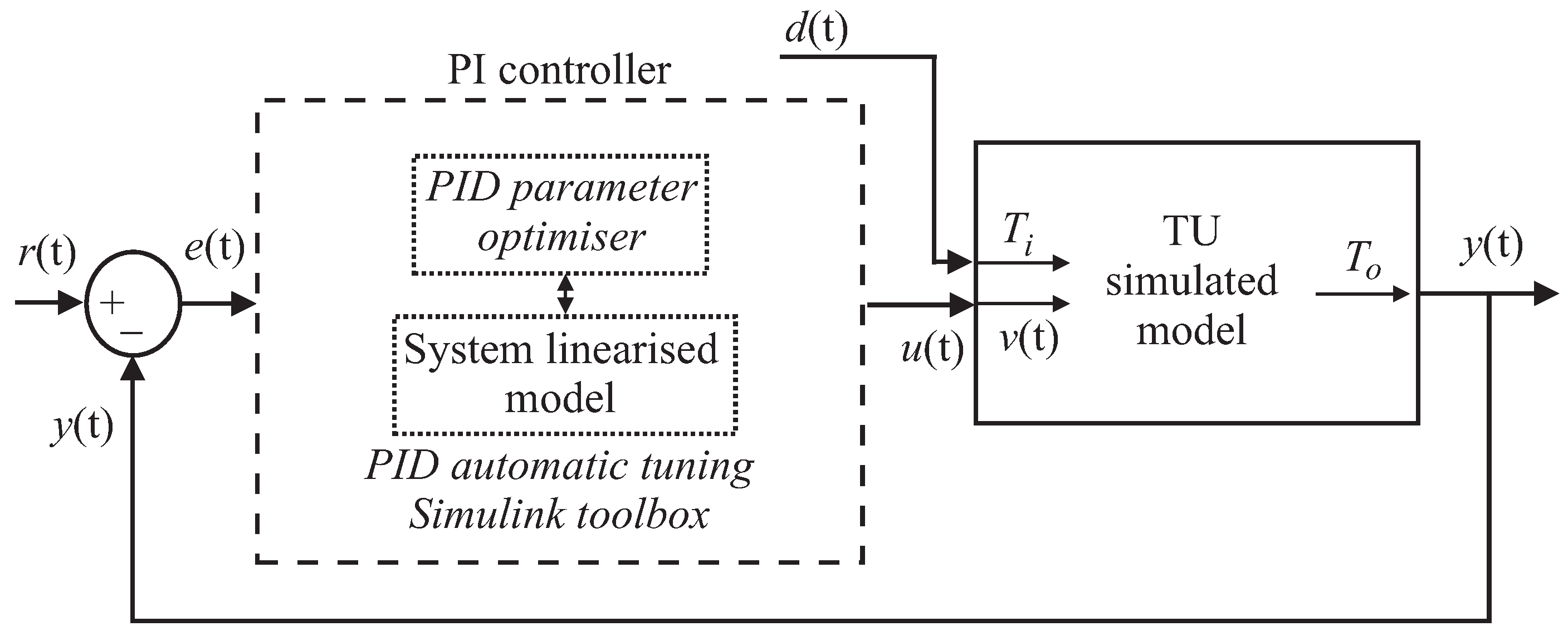
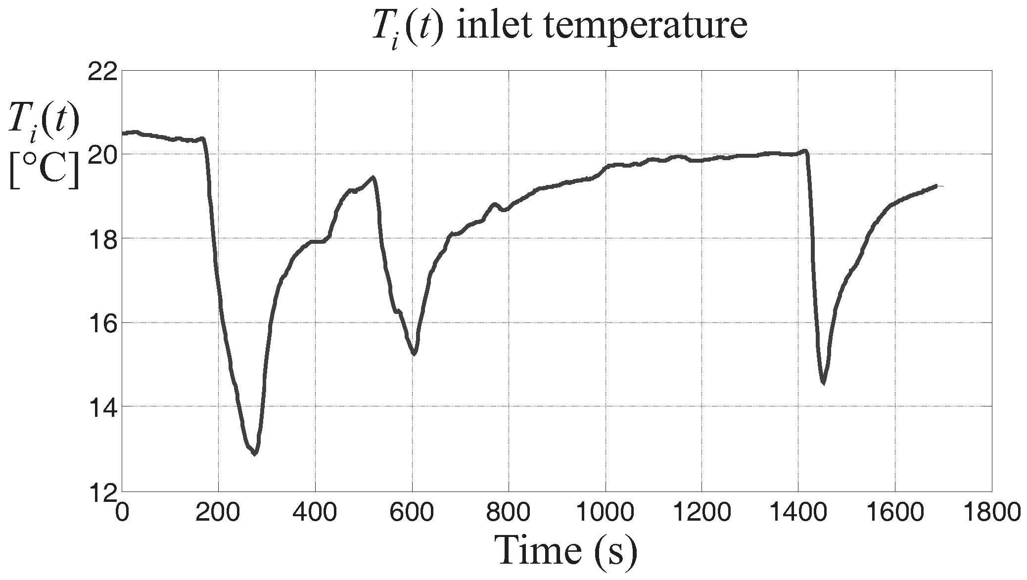
As already remarked, many HVAC systems are controlled via standard PID regulators. Therefore, the first results are achieved by exploiting a regulator in the form of Equation (6) applied to the TU simulated model as represented in Figure 3. Note that in the scheme of Figure 3, the control input $u\left(t\right)$ is the inlet air speed $v\left(t\right)$, whilst the inlet air temperature $T_i\left(t\right)$ is considered as measurable disturbance $d\left(t\right)$, which is shown in Figure 4.

With reference to this control strategy, the optimal controller gains are computed using the automatic PID tuning procedure from the PID Simulink^® block. The proportional, integral and derivative gains have been determined as $K_p=1.4465$, $K_i=0.0339$ and $K_d=0.4228$, respectively. The derivative filter time–constant has been estimated as $T_f=4.4034$.

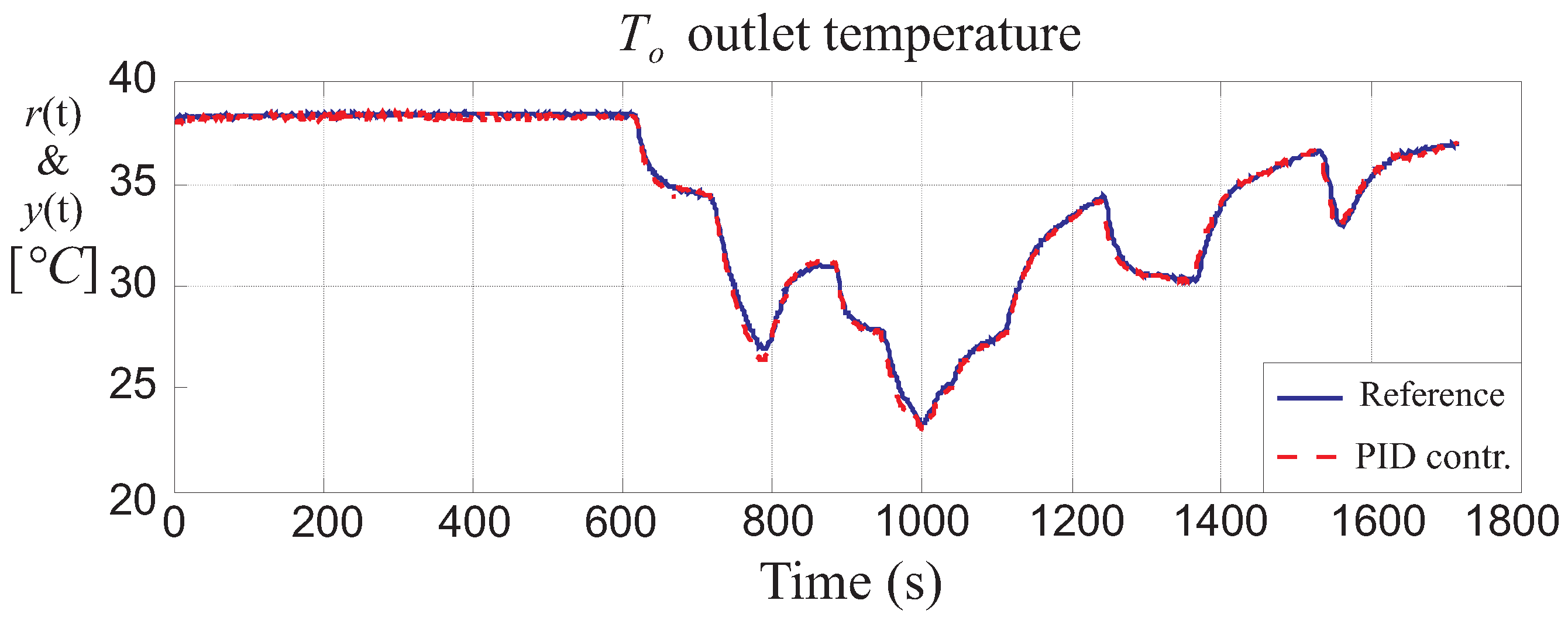
Figure 5 represents the set-point $r\left(t\right)$ (blue continuous line) and the TU measured output $y\left(t\right)=T_o$ (red dashed line) regulated via the PID standard controller. With this methodology, the PID regulator is able to guarantee a response with settling time $T_s=2.17$ s and maximum overshoot $S\%=36.14\%$. These values are derived by applying a step change in the reference signal $r\left(t\right)$ from 39 °C to 40 °C. The tracking error evaluated via Equation (21) is $MSSE\%=1.65\%$.

Note that the reference signal $r\left(t\right)$ considered for control purpose, i.e., the outlet air temperature $T_o\left(t\right)$ represented also one of the excitation signals exploited for the identification of the TU model described in [9]. Moreover, the authors have exploited this reference signal since it guarantees the correct working conditions and the validity of the identified model of Equation (4).

It is worth observing that PID standard controllers can provide sufficient robustness properties after a straightforward tuning phase, thus representing interesting and easy to use solutions with simple and viable implementation. However, despite these features, the achieved control laws might not be sufficiently efficient in terms, e.g., of energy consumption and maintenance costs, when applied to HVAC systems. Due to these possible limitations, the paper has investigated alternative control strategies for achieving improved performances. To this aim, the PID regulator obtained via the auto-tuning procedure is regarded as a reference controller for the computation of advanced and alternative control strategies.

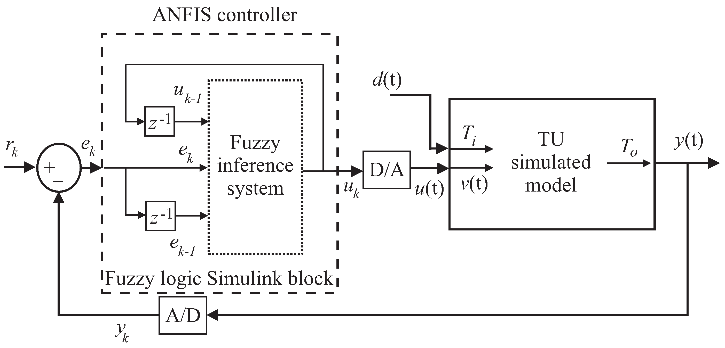
First, a TS fuzzy model of the controller has been derived using the fuzzy identification method recalled in Section 3.2. The procedure exploited the so-called model reference control (MRC) approach described, e.g., in [49]. In this way, the TS fuzzy controller is derived via the ANFIS tool, with a sampling interval $T=0.1$ s.

Figure 6 reports the diagram of this control solution, where this fuzzy regulator uses $K=3$ Gaussian membership functions and a number of delayed input and output samples $n=1$. Figure 6 highlights also that the antecedent vector of the ANFIS tool is $x\left(k\right)={\left[e\left(t_k\right),e\left(t_{k-1}\right),u\left(t_{k-1}\right)\right]}^T={\left[e_k,e_{k-1},u_{k-1}\right]}^T$.

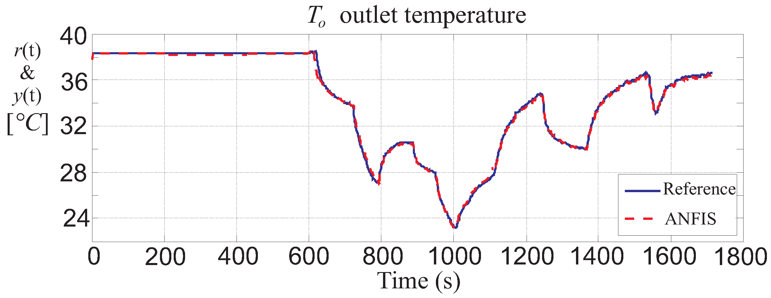
On the other hand, Figure 7 reports the achieved performance of the regulator obtained with the ANFIS tool by comparing the reference $r\left(t\right)$ (continuous blue line) and controlled output $y\left(t\right)$ (red dashed line). In this case, the settling time is $T_s=2.21s$, with a maximum overshoot $S\%=38.22\%$ and $MSSE\%=1.07\%$.

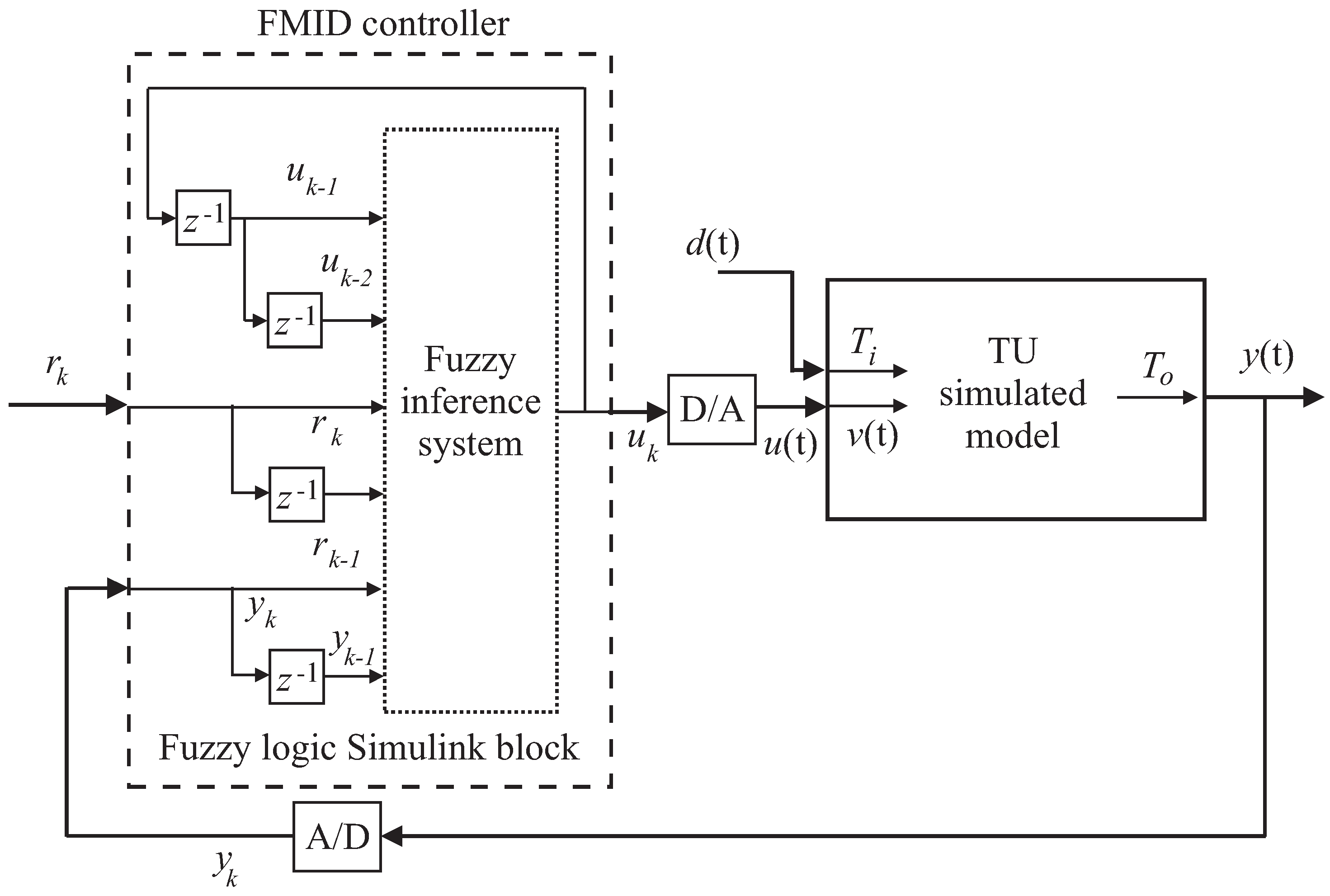
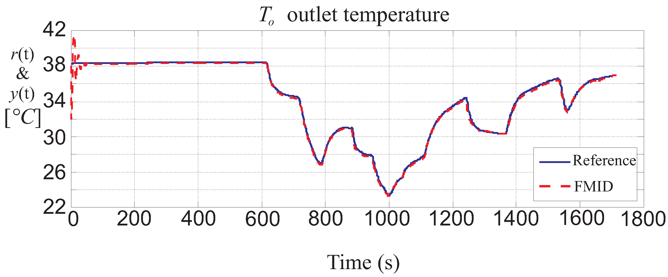
This work also proposes the derivation of a fuzzy controller in the form of Equation (11), whose structure and parameter estimation relies on the FMID tool. This tool is able also to provide the estimation of the fuzzy membership functions ${\mu }_{A_i}(.)$ in Equation (11).

Once the structure of this TS fuzzy regulator has been achieved, the obtained regulator is sketched in Figure 8, for an optimal number of clusters $K=3$ and delays $n=2$. For this fuzzy system, the antecedent vector is defined as $x\left(t_k\right)={\left[u\left(t_{k-1}\right),u\left(t_{k-2}\right),r\left(t_k\right),r\left(t_{k-1}\right),y\left(t_k\right),y\left(t_{k-1}\right)\right]}^T=$ ${\left[u_{k-1},u_{k-2},r_k,r_{k-1},y_k,y_{k-1}\right]}^T$.

The results achieved by this TS fuzzy regulator obtained via the FMID library of the MATLAB^® environment are summarised in Figure 9. In this situation, the set-point $r\left(t\right)$ (blue continuous line) is tracked with an $MSSE\%=1.14\%$. On the other hand, the step transient response presents a settling time $T_s=3.98$ s and a maximum overshoot $S\%=41.65\%$. Finally, it is worth nothing that the high overshoot at the beginning of the simulation in Figure 9 is due to the initial conditions of the delay blocks of the fuzzy controller represented in Figure 9 that are zero.

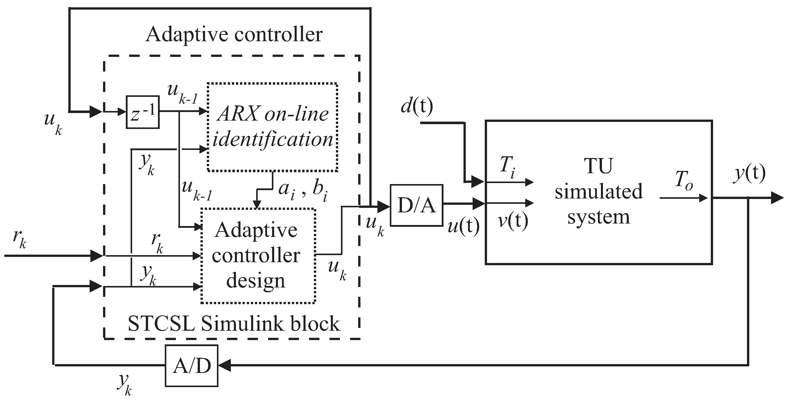
A further class of regulators has been considered in this work, and an adaptive controller has been developed according to the strategy recalled in Section 3.3.

The diagram of the adaptive compensator in the form of Equation (13) is shown in Figure 10, which is applied to the TU simulated model. The time-varying parameters of the difference model of Equation (12) have been recursively estimated by considering appropriate values of δ and ${\omega }_n$ in the polynomial $P\left(s\right)$ of Equation (16), which represent the damping factor and the natural resonance frequency of the closed-loop controlled system.

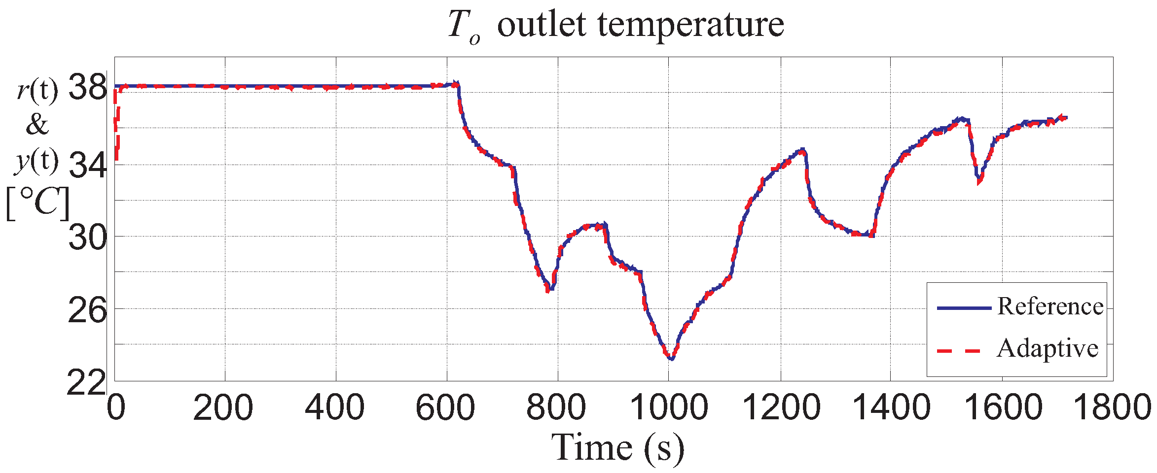
The tracking performances of the designed adaptive controller are summarised Figure 11. In particular, the settling time of the step transient response is $T_s=3.65$ s with a maximum overshoot $S\%=40.18\%$, whilst the achieved tracking error corresponds to an $MSSE\%=1.18\%$.

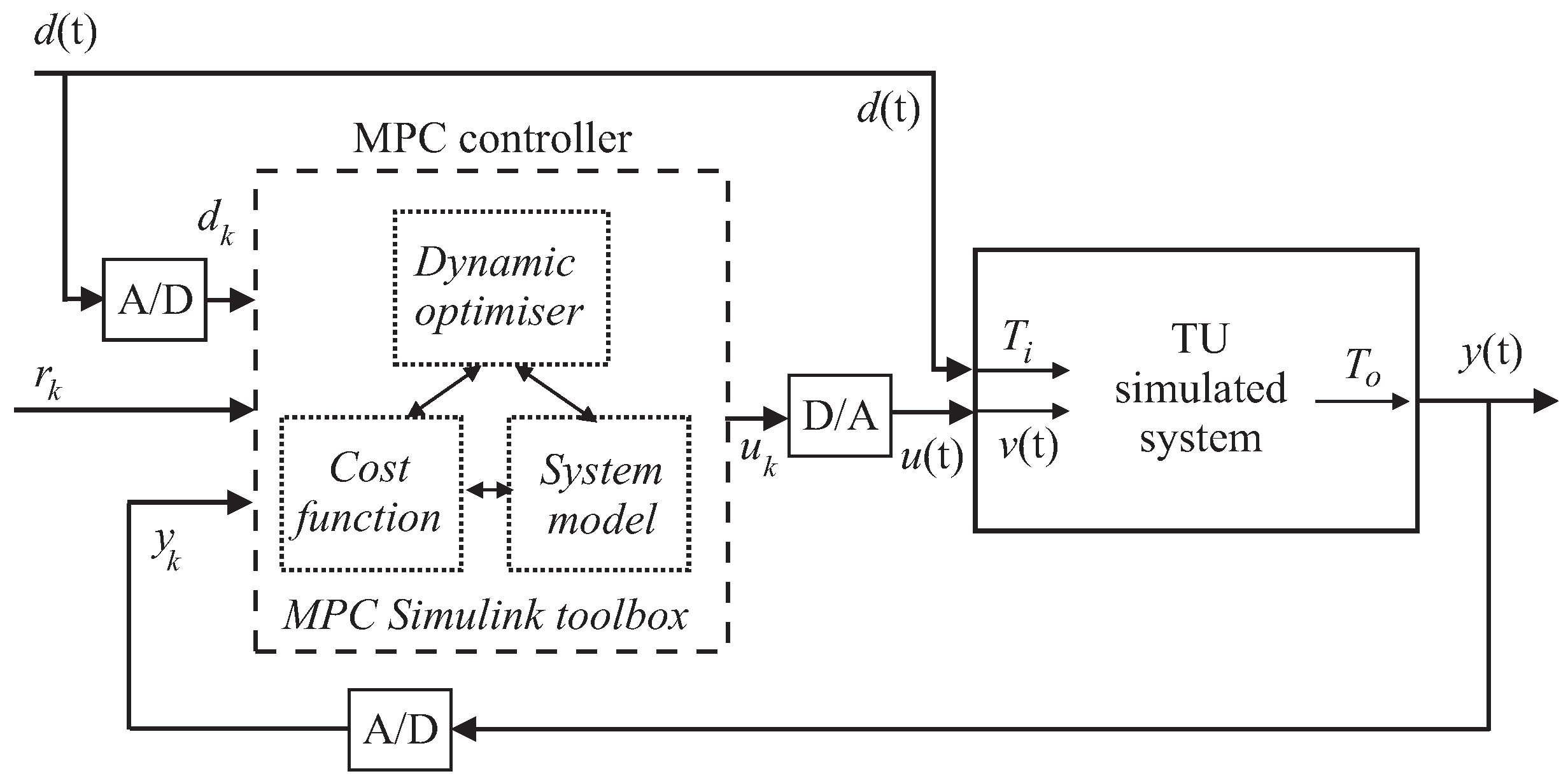
Finally, with reference to the MPC strategy summarised in Section 3.4, Figure 12 reports the block diagram of the MPC applied to the TU module via the D/A and A/D devices. The scheme of Figure 12 assumes that the disturbance signal $d\left(t\right)=T_i\left(t\right)$ can be measured and exploited by the MPC block.

It is worth noting that in this case, the MPC design exploits a prediction horizon of $N_p=10$ and a control horizon of $N_c=2$ for the minimisation of the cost function J of Equation (17). Moreover, the weighting coefficients of this cost function J are settled to $w_{y_k}=0.1$ and $w_{u_k}=1$ in order to minimise possible abrupt changes of the control input $u\left(t_k\right)$ that would increase the energy consumption and the controlled system efficiency.

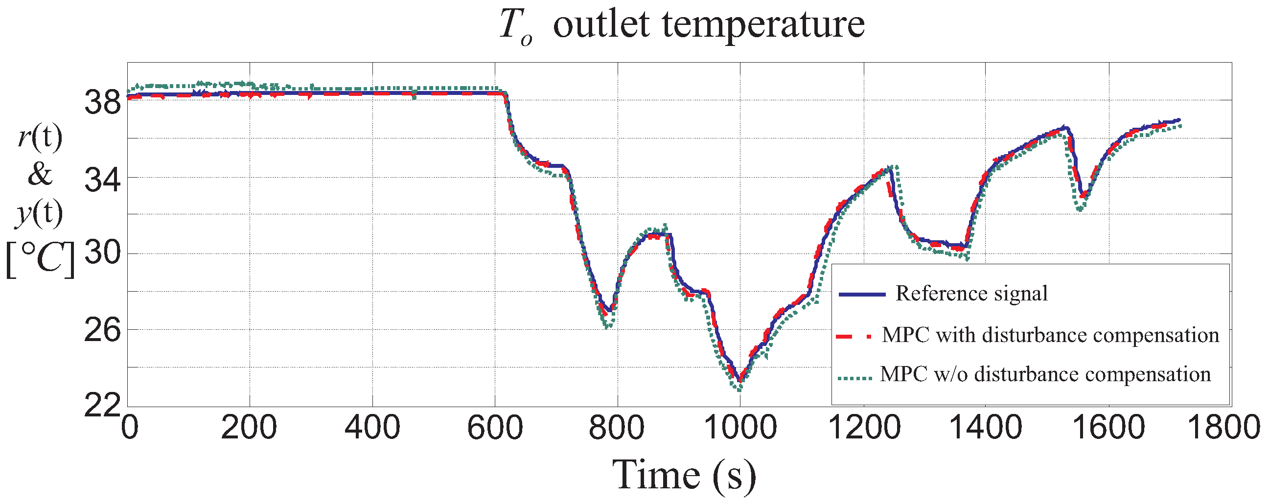
In this situation, as shown in Figure 13, the step transient response of the controlled TU module presents a settling time $T_s=1.85$ s and a maximum overshoot $S\%=35.51\%$, with a tracking error $MSSE\%=0.41\%$. Figure 13 shows also the results obtained with the MPC control using the linearised state-space model of Equation (19), when the disturbance $d\left(t\right)$ does not feed the MPC block of Figure 12.

Figure 13 highlights that the knowledge of the measured disturbance $d\left(t\right)$ that is exploited by the MPC block of Figure 12 improves the performance of the linear MPC strategy.

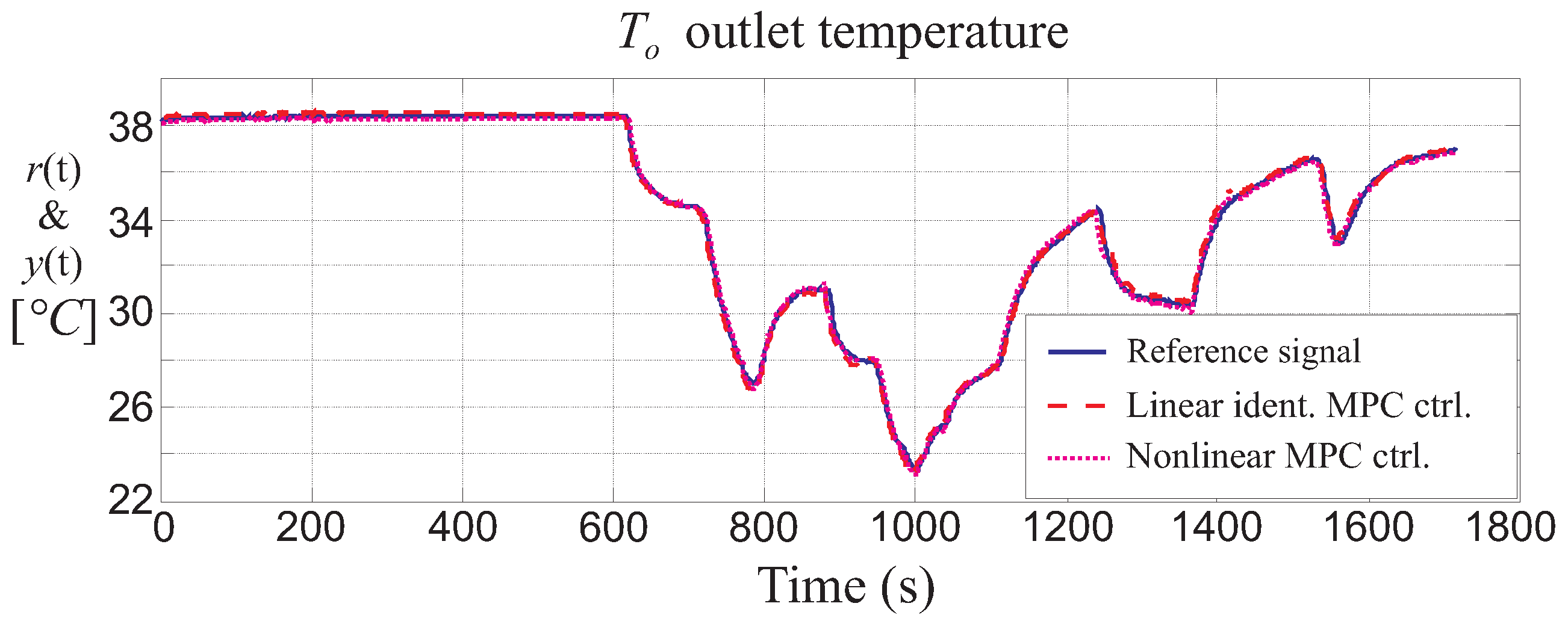
On the other hand, Figure 14 shows the comparison between the MPC design performed using the identified state-space model of Equation (20) and the nonlinear dynamic MPC scheme relying on a neural model of the controlled process sketched in Section 3.4.

Figure 14 highlights that the nonlinear MPC leads to slightly better results with respect to the linear MPC with the identified state-space model of Equation (20).

In order to analyse the obtained performance and compare the results achieved with the application of the control strategies proposed in this work,

Table 2. Performances with the proposed controllers.

Controller Type	Settling Time ${\mathit{T}}_{\mathit{s}}$	Overshoot $\mathit{S}\%$	Tracking Error $\mathit{MSSE}\%$
Auto-tuning PID	$2.17$ s	$36.14\%$	$1.65\%$
ANFIS Fuzzy	$2.21$ s	$38.22\%$	$1.07\%$
FMID Fuzzy	$3.98$ s	$41.65\%$	$1.14\%$
Adaptive	$3.65$ s	$40.18\%$	$1.18\%$
Linear MPC with disturbance compensation	$1.85$ s	$35.51\%$	$0.41\%$
Linear MPC w/o disturbance compensation	$1.97$ s	$37.64\%$	$1.27\%$
Linear MPC with identified model	$1.82$ s	$35.02\%$	$0.33\%$
Nonlinear MPC with identified neural model	$1.79$ s	$29.73\%$	$0.14\%$

summarises the features of these regulators in terms of step response settling time $T_s$, maximum overshoot $S\%$ and tracking error $MSSE\%$.

With reference to Table 2, the MPC schemes allow one to achieve the best performances with respect to the proposed indices. The superior results obtained by this control scheme seem to derive from the ability of the MPC methodology to anticipate future events, thus being able to take control actions accordingly. Moreover, the benefits of exploiting both an identified state-space model and a nonlinear prototype of the controlled process in connection with the knowledge of the measured disturbance $d\left(t\right)$ seem quite clear from the results reported in Table 2.

On the other hand, also the TS fuzzy controller derived via the ANFIS toolbox in connection with the MRC principle seems to present interesting features in terms of step response settling time, maximum overshoot and tracking error when compared to the other methodologies. This property can be due to the ANFIS strategy that relies on a fuzzy inference system. In fact, the ANFIS scheme includes the capabilities of both the neural network and the fuzzy logic tools, with the advantage of integrating their benefits in one whole structure. Moreover, as already observed, the proposed fuzzy approach that integrates learning capability is able to approximate the process nonlinear behaviour with an error depending on the required accuracy level. The adaptation strategy implemented in ANFIS presents interesting computationally-efficient features since it relies on genetic algorithms used to estimate the best model structure and its parameters [49].

Note, however, that the standard PID regulator leads to achieving the second best step response settling time since it exploits the auto-tuning scheme implemented in the Simulink^® PID block in order to optimise its parameters. This feature can represent an important aspect when a good trade-off between control performance and implementation simplicity is required. In general, the standard PID control law is usually based on the process controlled variable and not on the knowledge of the underlying process behaviour. However, on the one hand, an automatic tuning of its parameters allows the PID controller to manage general control requirements, also in terms of step response rise time, closed-loop bandwidth, maximum overshoot and system oscillation amplitude. On the other hand, PID controllers cannot guarantee any control optimality and, in some situations, the overall system stability, but provides a viable and easy-to-use tool for providing a simple control law with acceptable performance.

4.1. Control Solution Sensitivity Evaluation

This study has considered further simulations that are useful for analysing the reliability and robustness characteristics of the considered control solutions with respect to possible parameter variations. This approach represents a way for analysing the well-known model-reality mismatch issue that can represent a limitation of the achievable performance of the proposed controller designs.

To this aim, the Monte Carlo (MC) tool is the key point since the controller behaviour and the design strategy depend on this model-reality mismatch, which can derive, e.g., from the model nonlinearity and its approximation, the uncertainty and disturbance terms, as well as input and output measurement errors. Therefore, the MC analysis simulates the behaviour of the controlled TU model when its parameters are described as Gaussian variables with mean values equal to the nominal ones and standard deviations of $\pm 20\%$ of the corresponding parameter values.

Under these assumptions, the analysis of the closed-loop control schemes has been performed by computing the best, average and the worst values of the $MSSE\%$ index of Equation (21) evaluated over 500 MC runs. These values are summarised in

Table 3. $MSSE\%$ values obtained via the MC analysis for controller performance evaluation.

Control Scheme	$\mathit{MSSE}\%$ Best Case	$\mathit{MSSE}\%$ Worst Case	$\mathit{MSSE}\%$ Average Value
Auto-tuning PID	$1.44\%$	$3.14\%$	$1.65\%$
ANFIS Fuzzy	$1.03\%$	$2.33\%$	$1.07\%$
FMID Fuzzy	$1.10\%$	$2.47\%$	$1.14\%$
Adaptive	$1.06\%$	$1.78\%$	$1.18\%$
Linear MPC with disturbance compensation	$0.38\%$	$0.81\%$	$0.41\%$
Linear MPC w/o disturbance compensation	$0.97\%$	$1.98\%$	$1.27\%$
Linear MPC with identified model	$0.28\%$	$0.67\%$	$0.33\%$
Nonlinear MPC with identified neural model	$0.09\%$	$0.31\%$	$0.14\%$

.

On the basis of the results of Table 3, it seems clear that the MPC designs lead to the best performance when the modelling of the controlled system and the measured disturbance $d\left(t\right)=T_i\left(t\right)$ is taken into account. On the one hand, the MPC design can rely on the knowledge of a state-space model in the form of Equation (18), derived from both a linearisation procedure or an identification experiment. On the other hand, the MPC design can use an identified nonlinear model of the process, as remarked at the end of Section 3.4. The overall methodology is based on the optimisation of the cost function of Equation (17). However, once the description of the controlled process has been available as a linear or nonlinear dynamic model, the MPC design is quite simple and straightforward.

The control schemes relying on the ANFIS and the FMID tools can lead to interesting control performance, but with a learning phase that can be computationally heavy and time consuming, especially when the numbers of rules K, the antecedents and the model delays n are high.

Similar considerations hold for the adaptive controllers, which can track possible variations of the controlled model parameters, but with possibly complex design procedures required for computing the controller coefficients.

Standard PID regulators require simple design and simple implementation, but in general, they lead to limited performance, which can imply lower efficiency when applied, e.g., to HVAC systems. The same remarks are valid for the fuzzy controllers relying on AI tools, whose parameters can be easily estimated from the input-output data acquired from the controlled process. However, a further optimisation stage can be required, which sometimes is time consuming, but these fuzzy solutions can enhance the achievement of advanced performance indices.

It is worth observing that the MC methodology proposed in this work seems to represent the key point for the validation and the verification of the proposed control solutions when applied to the TU module in the presence of modelling and measurement errors, uncertainty and disturbance terms.

Note finally that the control methodologies followed by the analysis procedures shown in Section 3 and Section 4 are developed using the MATLAB^® and Simulink^® software tools, in order to automate the overall design and simulation phases. These feasibility and reliability studies are of paramount importance for real application of control strategies once implemented for future air conditioning system installations.

5. Conclusions

In this work, several data-driven and model-based control strategies were recalled, designed and applied to a nonlinear thermal unit model, which can be considered as a fundamental module of phase change material larger systems exploited in passive air conditioning devices. The feasibility of the obtained solutions and the reliability features of the proposed methodologies were analysed in simulation using the measurements acquired from a realistic test-rig of a passive air conditioning system. The Monte Carlo tool represented the practical method for validating the features of these control schemes in the presence of modelling, disturbance and measurement errors. The achieved results highlighted that the controllers designed for example with artificial intelligence schemes were able to provide interesting behaviour in terms of settling time, maximum overshoot and tracking error, even if the adaptation phase can be time consuming. Optimal results were obtained using the model predictive control methodology, even if the derivation of appropriate descriptions of the controlled process and the minimisation of a cost function are required. Finally, future works will investigate the control design and its application for the regulation of different comfort and health parameters of real air conditioning systems, such as the relative humidity, since they directly affect the air conditioning system operating costs in terms of energy.