1. Introduction
Modern power systems contain huge amounts of cyber devices, which form the cyber network to monitor, control and protect the physical network. The interdependence of the cyber network and physical network makes modern power systems typical cyber-physical systems, i.e., cyber-physical power systems (CPPS). However, the cyber layer in a CPPS brings new uncertainties while improving the power supply quality. Unexpected malfunctions in the cyber layer may lead to the loss of visibility and control of the physical layer, placing the CPPS at great risk. Supervisory control and data acquisition (SCADA)/energy management system (ENS) failures were major factors leading to the 2003 Italy blackout and 2003 Northeast blackout [
1,
2]. In addition, the Ukraine power grid suffered a blackout in 2015 due to hacker attacks, which shows that malicious attacks on CPPS may lead to more serious consequences [
3]. Therefore, it is necessary to research the impact of the cyber layer during the cascading failure process, and analyze the vulnerability of CPPS, especially the vulnerability of the cyber layer.
Multiple methods were introduced in [
4,
5,
6,
7,
8,
9,
10,
11] to assess the vulnerability of conventional power systems. These studies ignore the cyber layer and focus on physical layer vulnerability assessment. In the CPPS environment, such a consideration is not appropriate since the influence of the cyber layer is too great to ignore. Interdependences between cyber layer and physical layer should be analyzed. In the aspects of CPPS modeling and interdependence assessment, reference [
12] established a cyber-based dynamic model which had network structure-preserving properties that could improve the efficiency of distributed electric power system decision making. A cyber-physical equivalent model for a hierarchical control system (HCS) had been proposed in [
13]. The HCS network was abstracted to a node-branch graph using this model, and information flow was expressed by a series of mathematical equations for the sake of cyber-contingency assessment. Falahati et al. [
14,
15] discussed direct and indirect interdependencies in modern power systems, introduced a state mapping method to map the cyber layer failures to physical layer failures, and two optimization models were presented to minimize the losses. The impact of direct cyber-power interdependencies (DCPIs) was also studied in [
16], and risk assessment methods under different distributed generation (DG) scenarios were proposed. Reference [
17] incorporated WAMS malfunction in power system reliability assessment. The authors indicated that wide-area measurement system (WAMS) malfunctions might lead to power systems being unobservable and uncontrollable, which would prevent the operators from taking remedial actions. Lei et al. designed a typical IEC-61850-based protection system incorporating physical and cyber components, and developed the cyber-physical interface matrix (CPIM) which defined the relationship between the cyber subsystems and physical subsystems in terms of failure modes and effects [
18]. Then, the concepts were extended from substation to integrated system, and the consequent event matrix (CEM) was established to provide detailed information about affected transmission lines [
19]. The applications of CPIM and CEM could decouple the cyber part analysis from the physical part analysis, and provide a more tractable method for CPPS reliability assessment.
Considering the impact of the cyber layer, several studies have focused on vulnerability assessments of power systems. Zonouz et al. [
20] presented a security-oriented cyber-physical contingency analysis (SOCCA) framework to evaluate the impacts of both accidental contingencies and malicious attacks. Security indices were calculated for the power grid’s corresponding Markov decision process (MDP) model, and various security incidents were ranked for proactive intrusion prevention solutions. Vulnerabilities of SCADA systems at three levels—system, scenarios, and access points—were evaluated in [
21], and the impacts of a potential electronic intrusion were expressed by its potential loss of load in power systems. The result showed that a lower password policy threshold would lead to a lower probability of success for the intrusion attempts. Reference [
22] indicated that failures in one network might result in failures in the other networks, and the allocation of interconnecting links between physical nodes and cyber nodes would greatly infect the robustness of the entire system. Then, an optimum inter-link allocation strategy was characterized under the condition of unknown subsystem topology. Chen et al. [
23] proposed two models of hidden failures in protection systems, and analyzed the contribution of hidden failures to cascading failure. Risk indices of power system cascading collapse were set up, including bus isolated risk, load isolated risk, grid break-up risk and integrated system risk. Reference [
24] presented CPINDEX, a security-oriented stochastic risk management technique to calculate the vulnerability rank of cyber-physical contingencies. Considering cyber network configurations, power system topology and the interdependencies among them, stochastic Bayesian network models of the entire cyber-physical infrastructure were established, and the security level of the current cyber-physical state was calculated using a graph-theoretic algorithm. Huang et al. [
25,
26] studied the cascading failure process in CPPS using percolation theory, and presented a detailed mathematical analysis of cascading failure propagation. For interdependences in CPPS, Huang et al. made the following assumptions: a node can operate only if it has at least one inter link (a link that connects cyber node and physical node) with a node that functions. Based on the assumption, the fraction of nodes that could still function after the cascading failure was estimated. The results showed that there exists a threshold for the proportion of faulty nodes, above which the system collapses.
In the CPPS environment, with wide application of communication, computer and control technologies, operators have a clear view on the real-time state of the physical layer and are able to control it from control centers. The cyber layer and physical layer have various impacts on the other layer, and failures in one layer may cause and affect the cascading failure. Reference [
17] studied the impacts of monitoring/control functions on power systems, but did not take the cyber layer topology and properties into account, and the model is not precise enough. Reference [
25] made an assumption about interdependence in CPPS and proposed a cascading failure model which could simulate the failure propagation between two layers. However, the model did not consider the characteristics of power flow in the physical layer, and the assumption about interdependence was not quite reasonable. For example, substation automation systems (SAS), which are abstracted into cyber nodes, are usually equipped with an uninterruptible power supply (UPS). During the cascading failure process, cyber nodes won’t fail due to the lack of power supply even if related physical nodes fail. Besides, when related cyber nodes fail, physical nodes will be unobservable and uncontrollable, but these physical nodes may still operate if there is no disturbance to the current system state. Physical nodes won’t fail due to the lack of monitoring and control either. To describe the cascading failure process and identify the vulnerable parts in CPPS more comprehensively, this paper proposes a practical CPPS model based on complex network theory, and introduces a vulnerability analysis method incorporating information processing analysis and power flow analysis. Vulnerabilities under different cyber-physical interface strategies and attack strategies are analyzed and compared to provide suggests to CPPS planners and operators. The main contributions of this paper are summarized below:
Considering cyber layer topology, physical layer topology and cyber-physical interface strategy, the CPPS model is proposed based on complex network theory.
Incorporating information processing analysis and power flow analysis into topological analysis, a vulnerability analysis method is introduced to simulate the interactions between cyber layer and physical layer during the cascading failure process.
Two vulnerability indices are proposed from the perspective of both topology structure and network property, vulnerabilities under different conditions are analyzed and compared.
The remainder of this paper is organized as follows: a detailed CPPS model is proposed in
Section 2. In
Section 3, the consequences of cyber node failures are analyzed, and a CPPS vulnerability analysis method is introduced. Case studies and result analysis are presented in
Section 4. Finally,
Section 5 concludes the paper.
2. CPPS Modeling
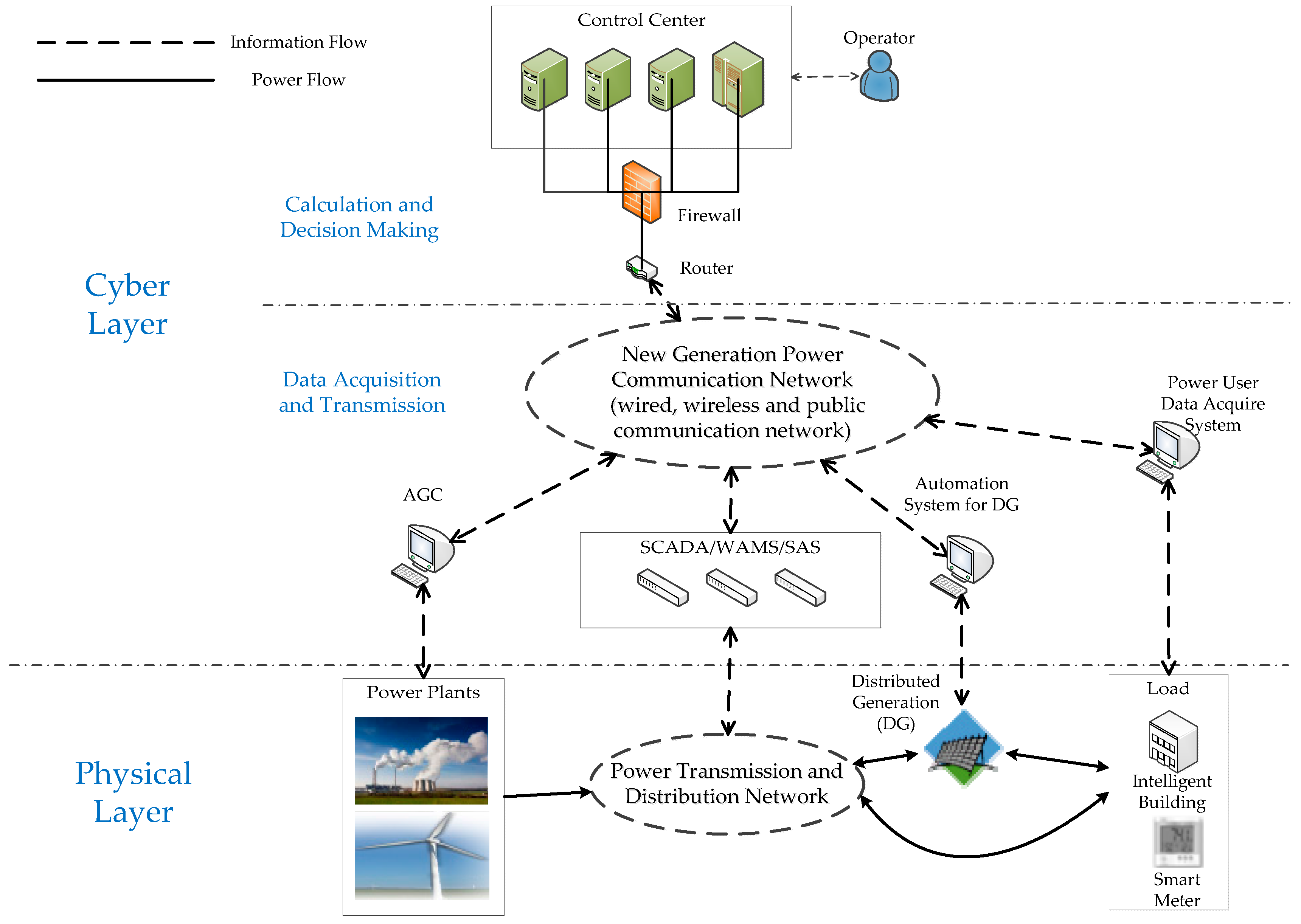
A CPPS consists of numerous cyber devices and physical devices, which form a cyber layer and a physical layer, respectively. The control center is in charge of calculation and decision making while the rest of the cyber layer is in charge of data acquisition and transmission. A typical CPPS structure is shown in
Figure 1. Based on the complex network theory, the whole CPPS can be abstracted into an undirected network which consists of cyber nodes, physical nodes and connections between them. The topological relationship of CPPS can be expressed by the CPPS adjacency matrix
. Assuming that the CPPS includes
cyber nodes
and
physical nodes
, the rank of
will be
, and the structure of
is as follows:
where
is the adjacency matrix of cyber layer which represents the connections inside cyber layer;
is the adjacency matrix of physical layer which represents the connections inside physical layer;
is the cyber-physical interface matrix which represents the interconnections between cyber layer and physical layer;
is the transposed matrix of
.
Obtaining of , and will be presented in the following subsections.
2.1. Cyber Layer Model
The cyber layer is an Ethernet-based communication network which monitors and controls the physical layer. Cyber nodes are the abstractions of cyber devices and related algorithms, such as SAS. Cyber edges are the abstractions of communications links. Scale-free network [
27] is a typical complex network which widely exists in the real world. A scale-free network is a network whose degree distribution follows a power law asymptotically. The main characteristic in a scale-free network is the distribution of the degree of node inhomogeneity. Massive amounts of data show that the Ethernet-based power system communication network is also a scale-free network. The Ethernet-based power system communication network can be divided into three layers: the core layer, the distribution layer and the access layer. The core layer and the distribution layer only include several nodes, but these nodes have much higher node degrees than nodes in the access layer. With the development of the network, more nodes would access the access layer and make degree distribution more inhomogeneous. For example, a double-star power system communication network is a scale-free network [
28]. Therefore, the cyber layer is considered to be a scale-free network, which can be modeled using the Barabási-Albert model. The modeling procedure is as follows:
After times, a scale-free network with nodes is established as the cyber layer of CPPS. is the adjacency matrix of the cyber layer network. The element in is 1 if there exists a cyber edge connecting cyber nodes and , otherwise is 0. Especially, .
A cyber node is the abstraction of a subsystem in the cyber layer instead of a specific cyber device, which are the set of all the related cyber devices and algorithms to monitor or control a physical node. Actually, cyber nodes can be seen as the automation systems of substations or power plants. It is noteworthy that one cyber node (or several) should represent the control center (power dispatch center). The high degree nodes in a scale-free network are often considered to serve specific purposes in their networks. Therefore, the node with the highest degree is considered to represent the control center.
Due to the properties of the cyber layer, the control center receives measurements, calculates and provides control commands but would cannot directly act on the physical layer. Therefore, the control center node should only be directly connected to other cyber nodes. Unless otherwise stated, the cyber nodes mentioned in the following of this paper mean other cyber nodes aside from the control center node.
2.2. Physical Layer Model
The physical layer is the current-carrying grid in CPPS, i.e., the conventional power system. Physical nodes are the abstractions of substations or power plants ignoring the internal structures inside them. Physical edges are the abstractions of transmission lines. For a given conventional power system structure, the physical layer model can be expressed by a complex network with physical nodes after these abstractions. is the adjacency matrix of physical layer network. The element in is 1 if there exists a physical edge connecting physical nodes and , otherwise is 0. Especially, .
2.3. Cyber-Physical Interface Strategy
There are various interdependences between the cyber layer and the physical layer. Cyber nodes require state data provided by the physical nodes, and physical nodes require control commands provided by the cyber nodes to operate safely. The corresponding relationship between cyber nodes and physical nodes could greatly affect the characteristics of the entire CPPS. Reference [
29] showed that different interface strategies of nodes in two networks have different influences on cascading failure processes between coupled networks, and proposed that the corresponding relationship of nodes in the two networks should have inter-similarity instead of randomness (i.e., nodes in two networks with similar topological properties tend to connect to each other).
In this paper, the cyber nodes and physical nodes are abstractions of subsystems instead of specific devices, and redundant devices inside a SAS would not affect the interconnection between cyber nodes and physical nodes. Therefore, we assume cyber nodes and physical nodes have a one-to-one correspondence (i.e., one cyber node only connects to one physical node and vice versa). To find out the optimal cyber-physical interface strategy to reduce the CPPS vulnerability, two cyber-physical interface strategies are analyzed and compared in this paper:
- (1)
Degree-betweenness interface strategy: This strategy states that cyber nodes with higher degrees and physical nodes with higher node betweennesses tend to connect to each other. The cyber nodes are sorted by node degree in descending order, and the physical nodes are sorted by node betweenness in descending order. Corresponding nodes in two sequences are connected by cyber-physical edges (i.e., the cyber node with highest degree is connected to the physical node with highest node betweenness, the cyber node with second highest degree is connected to the physical node with second highest node betweenness and so on). Cyber-physical edges are considered to be the abstractions of the interconnections between cyber layer and physical layer. For example, there are three cyber nodes
with degrees
and three physical nodes
with node betweennesses
, the cyber-physical edges should be
. Other degree and betweenness combination strategies are not considered, because reference [
30] already verified that the degree-betweenness interface strategy could reduce vulnerability more than others.
- (2)
Closeness centrality interface strategy: This strategy represents that cyber and physical nodes with higher closeness centrality tend to connect to each other. The cyber and physical nodes are all sorted by closeness centralities in descending order, and the corresponding nodes in two sequences are connected with cyber-physical edges (i.e., the cyber node with highest closeness centrality is connected to the physical node with highest closeness centrality, the cyber node with second highest closeness centrality is connected to the physical node with second highest closeness centrality, and so on). Closeness centrality [
31] is a node centrality index to measure the importance of a node, which can be expressed as follows:
where
represents the closeness centrality of node
;
is the set of nodes in network;
is the shortest distance from node
to node
.
is the cyber-physical interface matrix. The element in is 1 if there exists a cyber-physical edge connecting cyber node and physical node , otherwise is 0. Because control center node is not directly connect to physical nodes, all the elements of row in are 0.
3. CPPS Vulnerability Analysis Method
The cyber layer acquires the operation state of the physical layer as the input information. After evaluation and calculation, control commands are sent to the physical layer. The physical layer receives the control commands, and adjust its operation state to satisfy the economy and security. This closed-loop control could prevent a cascading failure. The failure control process in CPPS can be described by the following brief steps:
- Step 1:
A physical layer failure happens, the physical layer state changes from to .
- Step 2:
The physical layer state is acquired by cyber nodes through cyber-physical edges, and the acquired information is sent to the control center node through cyber layer network.
- Step 3:
In the control center node, the physical layer state is evaluated to judge whether the physical layer operates safely or not. If the evaluate result shows that there are limit violations in the physical layer, remedial actions should be calculated and generated.
- Step 4:
The remedial actions are sent to cyber nodes through the cyber layer network, then, sent to physical nodes through cyber-physical edges.
- Step 5:
The physical layer adjusts to a safely operation state according to the remedial actions. The initial physical layer failure is prevented from extending.
However, this process could face a critical problem when cyber nodes suffer from random failures or malicious attacks. In such situations, Step 2 and Step 4 will be influenced. If Step 2 is incorrect, part of the physical layer is unobservable to the control center node, and limit violations of the unobservable part cannot be known. Therefore, remedial actions may not be taken, and the violated component will eventually go off-line. If Step 4 is incorrect, part of the physical layer is uncontrollable, and parameters of the uncontrollable part cannot be dispatched. Therefore, the generated remedial action may not be the global optimal solution, and physical layer would suffer more losses.
3.1. Cyber Node Faliure Analysis
Due to the properties of the cyber layer, cyber nodes that cannot exchange information with the control center node and physical nodes are consider to be failed. Certainly, the cyber nodes that suffer from random failures or malicious attacks will directly fail. Besides, the cyber layer topology changes caused by the direct cyber node failure can cause more cyber nodes to lose communication with the control center node. Considering the cyber layer property and topology, the cyber nodes failure analysis is described as follows:
Choosing the direct failure cyber nodes. For each direct failure cyber node , remove all edges connecting to , i.e., set all the elements of row and column in the CPPS adjacency matrix to be 0.
Getting the cyber layer adjacency matrix from , calculate the shortest distance from cyber nodes to the control center node using Floyd-Warshall algorithm.
For each cyber node , if the shortest distance from to the control center node is infinity, is considered to be fail. Remove all edges connecting to , and modify the CPPS adjacency matrix .
3.2. Unobservable Consequence Analysis of Cyber Node Failure
The physical devices that can’t send their measurements to the control center are considered to be unobservable. The cyber-physical interface matrix
is obtained from the modified
in
Section 3.1. If all the elements of the
column in
are zeros, it means that physical node
has no cyber-physical edge, and the bus abstracted to
is unobservable. For a transmission line, if the two buses connected by this line are all unobservable, the line is also unobservable. All the limit violations in unobservable bus set
and unobservable line set
cannot be observed.
Making and represent the bus set and the line set respectively. Only if there are limit violations in or , remedial actions will be taken, otherwise, no remedial actions will be taken.
3.3. Uncontrollable Consequence Analysis of Cyber Node Failure
The physical devices that can’t receive control commands from the control center are considered to be uncontrollable. Due to the one-to-one correspondence of cyber nodes and physical nodes, the unobservable bus must be uncontrollable, and vice versa. Therefore,
can also represent the uncontrollable bus set, which is exactly the same as the unobservable bus set in
Section 3.2.
Remedial actions taken by operators are simulated by optimal power flow algorithm (OPF) [
32]. Assuming that the control center is aware of uncontrollable buses, the OPF is described as follows:
subject to:
where
is the load shedding of bus
;
,
are the injection active power and reactive power of bus
through lines;
,
are the active load and reactive load of bus
;
,
,
,
,
,
are the active power and reactive power output, lower limit, upper limit of generating unit in bus
, if bus
actually has no generating unit, these parameters are all 0;
,
are the power flow and power flow limit of line
;
,
,
are the voltage magnitude, voltage magnitude lower and upper limit of bus
;
,
are the increment of these parameters compared with the initial value before OPF;
and
are the bus set and the line set.
Equations (5)–(8) represent the bus active/reactive power balance constraint, transmission line power flow constraint and bus voltage constraint, which represent the properties of physical layer and will not change due to the cyber node failure. Equations (9)–(11) represent the generator active/reactive power constraint and load dispatch constraint, which will be affected by the cyber node failure. Equation (12) represents the uncontrollable consequence of cyber node failures. Several algorithm parameters become immutable, which may prevent the algorithm from converging to the global optimal solution and cause more loss in physical layer.
3.4. CPPS Vulnerability Index
The vulnerability of a system can be considered as the performance drop when a disruptive event emerges [
33]. The main mission of a CPPS is to continue to provide a power supply. Therefore, we need to analyze the vulnerability of CPPS from the perspective of network properties. Besides, the remaining topological structure after the cascading failure is also important for vulnerability analysis. The more complete the remaining topological structure is, the faster the system recovers from the failure status. Therefore, we also need to analysis the vulnerability of CPPS from the perspective of topological structure. For this purpose, two vulnerability indices are proposed: ratio of edge loss (ROEL) and ratio of load loss (ROLL), to represent the CPPS performance drop from the perspective of both topological structure and power supply:
where
and
represent the number of edges in the largest connected components of CPPS before and after the cascading failure caused by the disruptive event;
and
represent the sum of load on all buses before and after the cascading failure caused by the disruptive event.
3.5. Overall Procedure
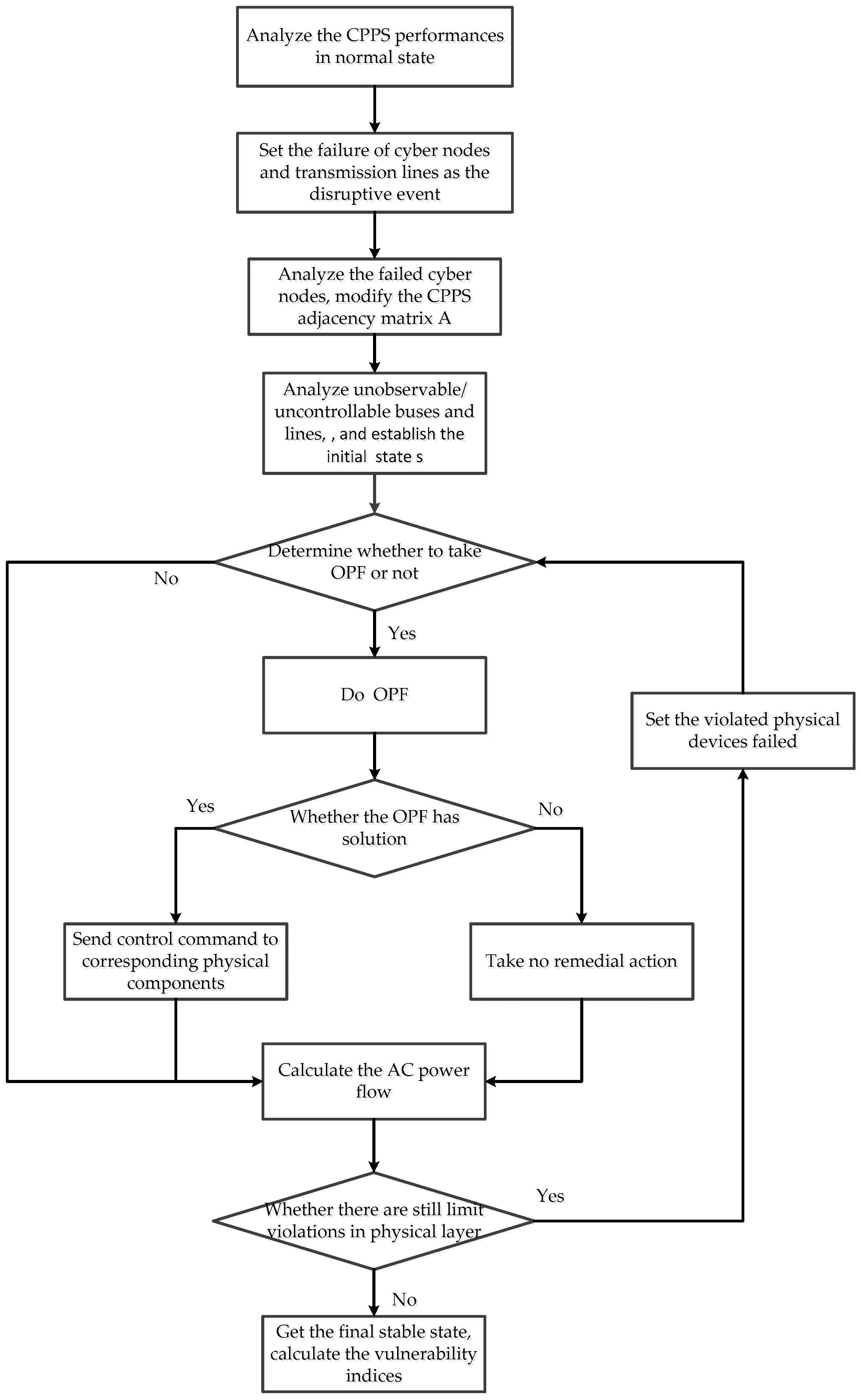
This paper proposed an analysis method to evaluate the vulnerability of CPPS. The flowchart of the proposed method is depicted in
Figure 2, and the overall procedure is summarized as follows:
- Step 1:
Analyze the CPPS performance in normal state, calculate and .
- Step 2:
Set the failure of cyber nodes and transmission lines as the disruptive event.
- Step 3:
Analyze the cyber node failures using the method mentioned in
Section 3.1.
- Step 4:
Establish the
and
using the method mentioned in
Section 3.2, and form the initial CPPS state
.
- Step 5:
Calculate the AC power flow, and check whether there are limit violations in and . If so, go to the next step; otherwise, go to Step 7.
- Step 6:
Do the OPF described in Equations (4)–(12). If the OPF has feasible solutions, set the optimal solution as the control commands which are sent to corresponding physical devices, and refresh the CPPS state; otherwise, take no remedial action.
- Step 7:
Calculate the AC power flow again, check whether there are still limit violations in and . If so, set the violated physical devices failed, refresh the CPPS state and return to Step 5; otherwise, go to the next step.
- Step 8:
Finish the cascading failure, calculate and and then, calculate the CPPS vulnerability indices ROEL and ROLL.
If the physical layer is split into several isolated islands during the procedure, Steps 5–7 should be applied to each island instead of the biggest island. Only if there are no limit violations in all islands, the cascading failure can be considered to be finished.
Step 3 represents the impact of cyber layer topological structure on cyber layer performance. Steps 5 and 6 represents the unobservable and uncontrollable consequences of cyber node failures. Step 7 actually simulates this violated physical devices failure process, if limit violations still exist in and , the violated physical devices will eventually fail. Violated lines will be tripped, violated buses will fail and all the generators and load on it will be lost.
4. Case Study
The test system is modified from the IEEE 57-bus system. The physical layer of the test system is abstracted from the IEEE 57-bus system. The power flow limit of a transmission line is set to two times the initial power flow, which is shown in
Table A1. Then, we take an economic dispatch for the physical layer and set the result as the normal state
. The cyber layer of the test system is a 58-node scale-free network which is generated using the method mentioned in
Section 2.1, and the sparse expression of
is shown in
Table A2.
The degrees and closeness centralities of cyber nodes, the betweennesses and closeness centralities of physical nodes are calculated and presented in
Table A3 and
Table A4, respectively. Cyber node
has the highest node degree 21. Therefore,
is considered to represent the control center, and the other 57 cyber nodes are considered to represent the automation systems of substations and power plants. The cyber-physical interface matrixes under two interface strategies are shown in
Table A5 and
Table A6, respectively.
The disruptive event of CPPS consists of two parts: transmission line failures and cyber node failures. For transmission line failures, we only consider the N − 1 contingencies. The consideration of cyber node failures will be discussed in
Section 4.2.
4.1. Scenario Analysis
To illustrate the proposed method more clearly, we assume cyber layer and physical layer are connected with degree-betweenness interface strategy in this subsection, and apply the proposed method on the following three typical scenarios:
- Scenario 1:
Line 13–15, connecting and , is failed without cyber node failures.
- Scenario 2:
Line 13–15 is failed while cyber node is failed due to malicious attacks.
- Scenario 3:
Line 13–15 is failed while cyber nodes , , , , and are failed due to malicious attacks.
Scenario 1 simulates the failure control process in CPPS while the whole cyber layer is functioning normally. After Line 13–15 is failed, the power flow on Line 9–13 is 8.98 MVA while the limit of Line 9–13 is only 6.07 MVA. A limit violation is observed and the OPF algorithm is used to control the failure. The OPF result shows that it is only need adjusting generator outputs without load shedding to eliminate the limit violation. After the physical layer receives the control commands, CPPS is in a stable state again and the cascading failure is prevented. In this scenario, ROEL is 0.0040 and ROLL is 0. The generator outputs before and after the remedial action are shown in
Table 1.
Scenario 2 simulates the uncontrollable consequences of a cyber node failure. When cyber node
is failed, Bus 8, which is abstracted to physical node
, is unobservable and uncontrollable. After the Line 13–15 outage happens and the limit violation of Line 9–13 is observed, although the OPF algorithm is activated, the parameters of Generator 5 located in Bus 8 cannot be dispatched in the optimization algorithm. In this scenario, the result shows that it requires not only adjusting generator outputs but also load shedding to eliminate the limit violation. The load on Bus 49 is curtailed from 18 MW to 16.83 MW. In this scenario, ROEL is 0.0280 and ROLL is 0.0009. The generator outputs before and after the remedial action are shown in
Table 2.
Scenario 3 simulates the unobservable consequence of cyber node failure. The initial failure may cause cascading failure, and physical layer may split into several isolated islands and suffer greater loss. When cyber nodes , , , , and are failed, Buses 9, 13, 19, 20, 21 and 22, which are abstracted to physical nodes , , , , , , are unobservable and uncontrollable. Therefore, Lines 9–13, 19–20, 20–21, 21–22 are also unobservable. After the Line 13–15 outage happens, the limit violation of Line 9–13 cannot the observed, so no remedial action will be taken and Line 9–13 will eventually fail. Then, Lines 19–20, 20–21 and 21–22 will fail one by one due to the unobservable consequences of cyber node failures. At this moment, Buses 20 and 21 have be split from the main island. Although the main island is in a stable state, the entire 2.3 MW load on Bus 20 is lost. In this scenario, ROEL is 0.1840 and ROLL is 0.0018.
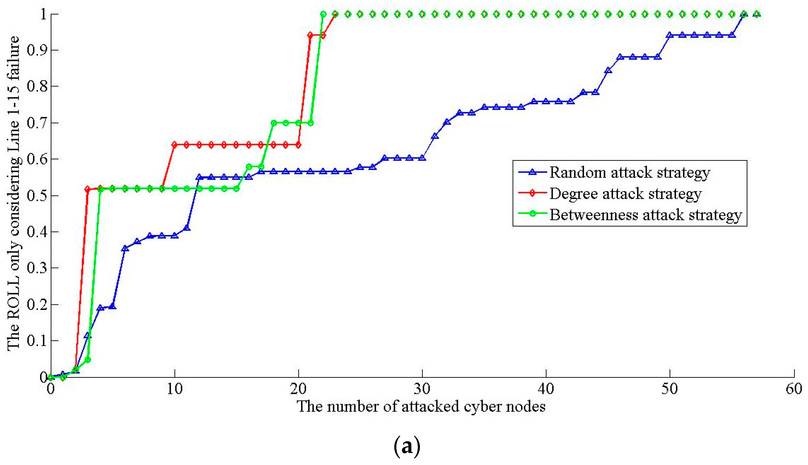
4.2. Attack Strategy Comparision
The vulnerabilities of CPPS under different attack strategies are different, so it is necessary to identify the attack strategy that is most dangerous to CPPS. Assuming the CPPS is modeled with degree-betweenness interface strategy in this subsection, we consider the following three possible attack strategies:
- (1)
Random attack strategy: The cyber node attack sequence is sorted randomly, the number of attacked cyber nodes increases from 0 to 57 gradually (i.e., the first attacked cyber node is selected randomly from all the cyber nodes, the second attacked cyber node is selected from the other cyber nodes except the first attacked cyber node, and so on). In order to guarantee the accuracy, we repeat the simulation 10 times and use the average value as the final result.
- (2)
Degree attack strategy: The cyber node attack sequence is sorted by node degrees in descending order, the number of attacked cyber nodes increases from 0 to 57 gradually (i.e., the first attacked cyber node is the cyber node with highest degree, the first attacked cyber node is the cyber node with second highest degree, and so on).
- (3)
Betweenness attack strategy: The cyber node attack sequence is sorted by node betweennesses in descending order, while the number of attacked cyber nodes increases from 0 to 57 gradually (i.e., the first attacked cyber node is the cyber node with highest node betweenness, the first attacked cyber node is the cyber node with highest node betweenness, and so on).
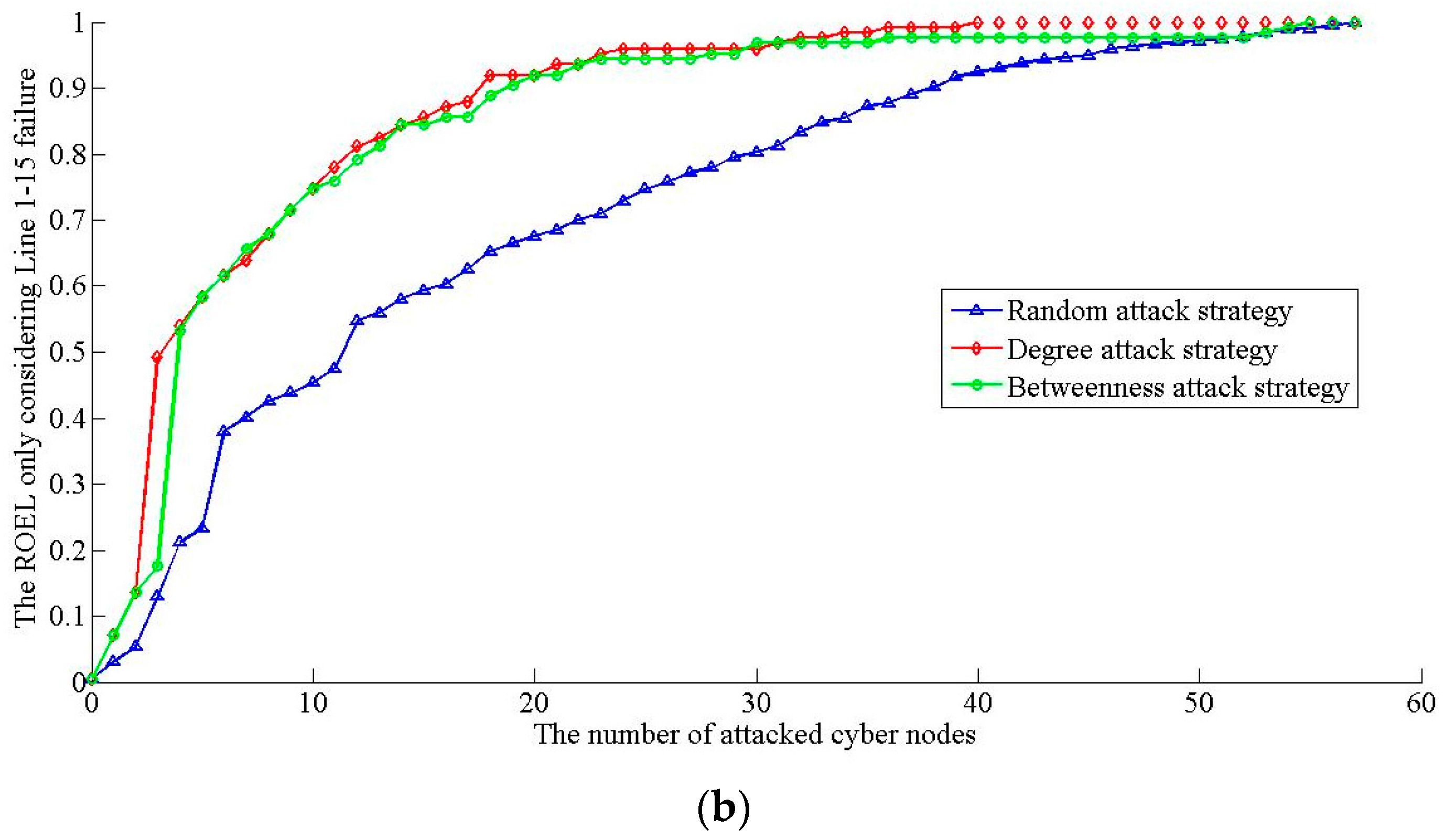
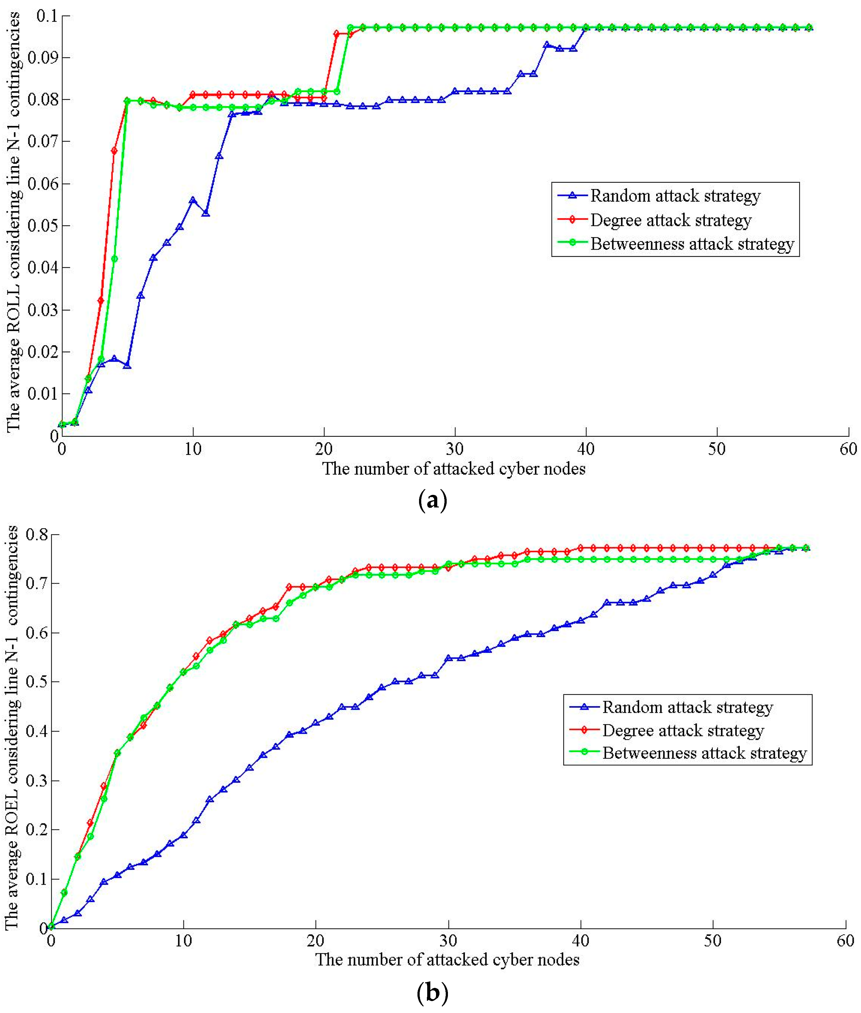
Under different attack strategies, the vulnerability indices of CPPS only considering Line 1–15 failure are shown in
Figure 3, and the average vulnerability indices of CPPS considering line N − 1 contingencies are shown in
Figure 4.
The results in
Figure 3 and
Figure 4 show that CPPS is more vulnerable when suffering malicious attacks than random attacks. Because the cyber layer of CPPS is considered as a scale-free network, there are only several high degree cyber nodes. These cyber nodes are key nodes. When suffering random attacks, as long as these key nodes are still functioning, the whole system will maintain a high performance. The failures of key nodes could greatly damage the structure of the cyber layer, and make more physical nodes unobservable and uncontrollable. Once a line outage happens, it is can easily develop into a cascading failure. The curves of ROEL and ROLL are not similar, which means that influences of a disruptive event on topological structure and network performance are different. It is necessary to analyze the vulnerability of CPPS from both perspectives.
From both
Figure 3a and
Figure 4a, we can see that there are two sudden changes in the ROLL curves. The first sudden change reflects the unobservable consequence of cyber node failures. Because the first several steps of cascading failure cannot be observed, the affected area will extend fast and more load will be lost. The second sudden change reflects the uncontrollable consequence of cyber node failures. Although the physical layer has split into several isolated islands, some islands may be still able to function alone. However, to ensure the frequency stability, the generators or load in a functioning island must be controllable. With more cyber nodes being attacked, the isolated islands will be totally uncontrollable and eventually collapse.
The attacked cyber node number of two sudden changes can be seen as two thresholds which can be used to value the CPPS vulnerability roughly. From
Figure 4a, we can determine that the two thresholds under degree attack strategy are 5 and 21, and the two thresholds under betweenness attack strategy are 5 and 22. The result means a degree attack strategy is more dangerous to CPPS.
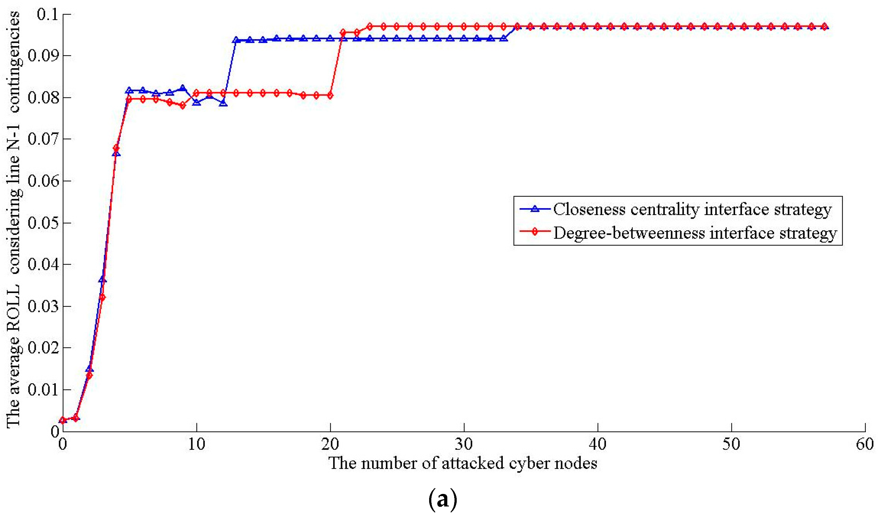
4.3. Cyber-Physical Interface Strategy Comparision
Since the scale-free property of cyber layer gives the CPPS great robustness against random attacks, we should find out the optimal cyber-physical interface strategy against malicious attacks. In this subsection, we assume a degree attack strategy is used, and compare the two cyber-physical interface strategies introduced in
Section 2.3. The average vulnerability indices of CPPS considering line N − 1 contingencies are shown in
Figure 5.
Although the ROEL curves of the different interface strategies are quite similar, the ROLL curves are quite different. The second threshold of the CPPS using closeness centrality interface strategy is smaller. When the CPPS is modeled using different cyber-physical interface strategies, the same cyber node may be connect to different physical nodes. If the same cyber nodes fail, the unobservable/uncontrollable physical area is different, and the performance drops of CPPS are certainly different. The two thresholds of CPPS using closeness centrality interface strategy are 5 and 13, while the two thresholds of CPPS using degree-betweenness interface are 5 and 21. Therefore, degree-betweenness interface is better than a closeness centrality interface strategy.
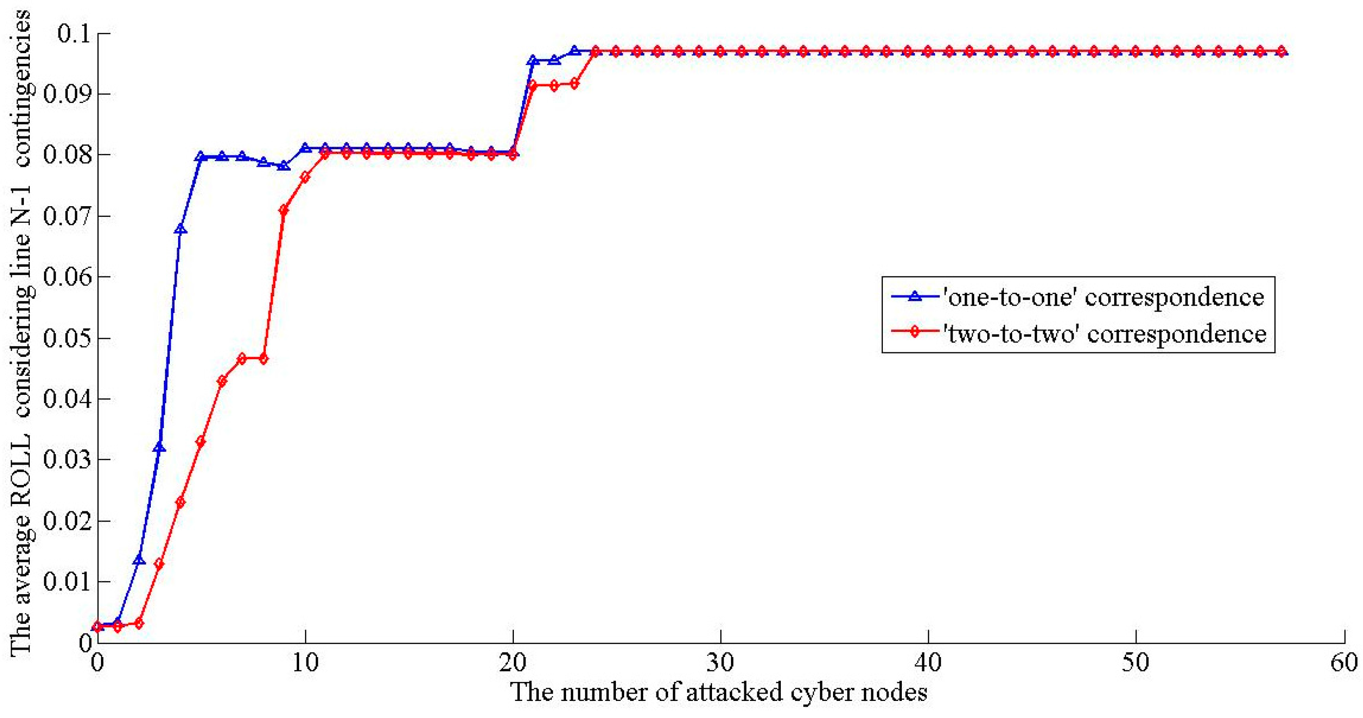
4.4. Additional Cyber-Physical Interconnections Analysis
In the previous analysis, a substation is considered to exchange data only with its own SAS, which means cyber nodes and physical nodes have a one-to-one correspondence. With the development of communication, computer and control technologies, the extra data exchange links from a substation to another substation’s SAS through a public network or a wireless network may be both technically and economically possible. The interconnections between cyber nodes and physical node could be extended into “two-to-two”.
In this subsection, we assume degree-betweenness interface is used. That is, the physical node with highest node betweenness is connected to the cyber nodes with the highest and second highest degree, the physical node with the second highest node betweenness is connected to the cyber nodes with the second highest and third highest degree and so on. The impacts of additional cyber-physical interconnections under a degree attack strategy are shown in
Figure 6.
The result in
Figure 6 shows that additional cyber-physical interconnections could effectively decrease the vulnerability of CPPS. The first threshold of “two-to-two” correspondence is 11, which is much bigger than the first threshold of “one-to-one” correspondence. Alse, the ROLL change is more gentle with additional cyber-physical interconnections. When the CPPS suffers a comparatively slight attack, only several cyber nodes fail. Due to the additional interconnections, the whole CPPS structure is more integrated and the cascading failure could be controlled more quickly. However, when the CPPS suffers a heavy attack, even the additional interconnections could not prevent the whole system from collapsing, and the two curves are similar after the first threshold. Therefore, additional interconnections could greatly decrease the vulnerability of CPPS, especially when facing slight threats.
5. Conclusions
Due to the interdependencies of the cyber layer and the physical layer, failures in the cyber layer may affect the behavior of the physical layer. During the cascading failure process, the lack of observations and control will accelerate the failure propagation and lead to greater losses. Therefore, it is necessary to analyze the vulnerability of CPPS and reinforce the weak points.
Against this background, this paper proposes a CPPS model which consists of a cyber layer, a physical layer and a cyber-physical interface, based on complex network theory. Considering the power flow properties, the unobservable and uncontrollable consequences of cyber node failure are discussed, and a CPPS vulnerability analysis method is proposed. Vulnerability indices are established from the perspectives of both topological structure and power supply. The initial failure of cyber node transmission lines is set as the disruptive event, and the cascading failure process caused by this disruptive event is simulated using the proposed method. The CPPS performance before and after cascading failures is compared, and the vulnerability of CPPS is analyzed. In the case study, two thresholds are proposed to roughly evaluate the CPPS vulnerability. The results show that CPPS is more vulnerable under malicious attacks, especially a degree attack strategy, and degree-betweenness interface is better in a closeness centrality interface strategy. The results also point out that cyber nodes with high degrees are key nodes. Improving the security of key nodes could reduce the CPPS vulnerability with minimum cost.
The model and method proposed in this paper are valuable to analyze the vulnerability in CPPS. Because of the complexity of CPPS, this paper makes some simplifications during the cascading failure simulation. In future studies, more factors should be taken into consideration, such as multi-level control center strategy, communication congestion, communication delay and hidden failures of the protection systems.


