Newton Power Flow Methods for Unbalanced Three-Phase Distribution Networks

Abstract

Two mismatch functions (power or current) and three coordinates (polar, Cartesian and complex form) result in six versions of the Newton–Raphson method for the solution of power flow problems. In this paper, five new versions of the Newton power flow method developed for single-phase problems in our previous paper are extended to three-phase power flow problems. Mathematical models of the load, load connection, transformer, and distributed generation (DG) are presented. A three-phase power flow formulation is described for both power and current mismatch functions. Extended versions of the Newton power flow method are compared with the backward-forward sweep-based algorithm. Furthermore, the convergence behavior for different loading conditions, $R/X$ ratios, and load models, is investigated by numerical experiments on balanced and unbalanced distribution networks. On the basis of these experiments, we conclude that two versions using the current mismatch function in polar and Cartesian coordinates perform the best for both balanced and unbalanced distribution networks.

1. Introduction

The electrical power system is one of the most complex system types built by engineers [1]. Traditionally, electricity was generated by a small number of large bulk power plants that use coal, oil, or nuclear fission and was delivered to consumers through the power system in a one-way direction. Due to the modernization of the existing grid, a large number of new grid elements and functions including smart meters, smart appliances, renewable energy resources, and storage devices are being integrated into the grid. Thus, the existing electrical grid is changing rapidly and becoming more and more complex to control. A smart grid (SG) is offered as the solution to this problem [2,3,4].

In a smart grid, most of the new grid elements are directly connected to the distribution network which requires new types of operation and maintenance. The distribution network has been considered as a passive network that totally depends on the transmission network for control and regulation of system parameters. Conventionally, the power flow in the distribution system was one-way traffic (vertical) from the substation (only source) to the end of the feeders. However, the utilization of distributed generation (DG) made the distribution network active in the sense that the distribution network can generate electrical power in the network and transfer the extra power to the transmission network. This changes the direction of the power flow in networks into two-way traffic (horizontal). Therefore, central grid operators or transmission system operators (TSOs) of the power system must have different approaches for maintaining and operating the electrical grid because in this case, the main purpose of the operator has been adjusted to interconnect the various active distribution networks. As the distribution network becomes more active, there is an increasing role of distribution system operators (DSOs). For efficient operation and planning of the power system, it is essential to know the system steady state conditions for various load demands.

A power flow computation that determines the steady state behavior of the network is one of the most important tools for grid operators. The solution of power flow computation can be used to assess whether the power system can function properly for the given generation and consumption. Traditionally, power flow computations were calculated only in the transmission network and the distribution networks were aggregated as buses in the power system model. However, in the new operation and maintenance of the distribution network, the power flow problem computation must be done on the distribution network as well.

A reliable distribution power flow solution method will be required to solve a three-phase power flow problem in unbalanced distribution networks integrated with distributed generations and active resources (i.e., renewable power generations, storage devices, and electric vehicles etc.) [5,6]. There are conventional power flow solution techniques for transmission networks, such as Gauss–Seidel (GS), Newton power flow (NR), and fast decoupled load flow (FDLF) [7,8,9] which are widely used for power system operation, control and planning. However, these conventional power flow methods do not always converge when they are applied to the distribution power flow problem due to some special features of the distribution network:

• Radial or weakly meshed (radial network with a few simple loops) structure:
  In general, a transmission network is operated in a meshed structure, whereas a distribution network is operated in a radial structure where there are no loops in the network and each bus is connected to the source via exactly one path.
• High $R/X$ ratio:
  Transmission lines of the distribution network have a wide range of resistance R and reactance X values. Therefore, $R/X$ ratios in the distribution network are relatively high compared to the transmission network.
• Multi-phase power flow and unbalanced loads:
  A single-phase representation is used for power flow analysis on transmission network which is assumed to be a balanced network. Unlike the transmission network, a distribution network must use a three-phase power flow analysis due to the unbalanced loads.
• Distributed generations:
  Unlike conventional power plants connected to the transmission network, DGs have fluctuating power output that is difficult to predict and control since it is strongly dependent on weather conditions.

Systems with the above features create ill-conditioned systems of nonlinear algebraic equations that cause numerical problems for the conventional methods [10,11,12]. Many methods have been developed on distribution power flow analysis and generally they can be divided into two main categories as:

• Modification of conventional power flow solution methods [13,14,15,16,17,18,19,20,21,22,23,24,25,26,27,28,29,30,31,32,33]:
  Methods in this category are generally a proper modification of existing methods such as GS, NR and FDLF.
• Backward–forward sweep (BFS)-based algorithms [34,35,36,37,38,39,40,41,42,43,44,45,46,47,48,49,50,51,52,53,54,55,56,57,58,59,60,61]:
  BFS-based algorithms generally take an advantage of the radial network topology. The method is an iterative process in which at each iteration two computational steps are performed, a forward and a backward sweep. The forward sweep is mainly the node voltage calculation and the backward sweep is the branch current or power, or the admittance summation.

Several reviews on distribution power flow solution methods can be found in [5,6,62,63,64].

In this paper, we focus on the Newton based power flow methods for balanced and unbalanced distribution networks with a general topology. Depending on the problem formulation (power or current mismatch) and specification of the coordinates (polar, Cartesian and complex form), the Newton–Raphson method can be applied in six different ways as a solution method for power flow problems. We refer to [65] for more details on all six versions of the Newton power flow method. In [65], the existing versions of the Newton power flow method [8,18,66] are compared with the newly developed/improved versions of the Newton power flow method (Cartesian power mismatch, complex power mismatch, polar current mismatch, Cartesian current mismatch, and complex current mismatch) for single-phase power flow problems in balanced transmission and distribution networks. It is concluded in [65] that the newly developed/improved versions have better performance than the existing versions of the Newton power flow method.

Therefore, we want to extend the Newton power flow methods developed for a single-phase problem in [65] to three-phase power flow problems. In this paper, only the polar current mismatch version is explained in detail for a three-phase power flow problem and the remaining versions can be derived similarly. Moreover, all six versions are implemented and compared with the BFS algorithm [43] for both balanced and unbalanced distribution networks. Different load models, loading conditions, and $R/X$ ratios are considered in order to analyze the convergence ability of all extended versions. The key contribution of this work is new formulations of the Newton power flow method. Compared to existing versions of the Newton power flow method, our versions use different equations for PV buses in the Jacobian matrix that result in better convergence and robust performance. We present how these versions can be applied to unbalanced distribution networks by studying loads, three-phase load connections, three-phase transformers, and DGs.

This paper is structured as follows. In Section 2, mathematical models of the power system, load, three-phase load connection, three-phase transformer, and DG are introduced. Section 3 mathematically describes the three-phase power flow problem. The Newton power flow method, the polar and the current mismatch formulations, and the polar current mismatch version are explained for the three-phase power flow problem in Section 4. The comparison result of all the versions of the Newton power flow method with BFS algorithm in balanced and unbalanced distribution networks is presented in Section 5. Finally, the conclusions are given in Section 6.

2. Power System Model

Power systems are modeled as a network of buses (nodes) and branches (transmission lines), whereas a network bus represents a system component such as a generator, load, and transmission substation, etc. There are three types of network buses such as a slack bus, a generator bus (PV bus) and a load bus (PQ bus). Each bus in the power network is fully described by the following four electrical quantities:

• $|V_i|$ : the voltage magnitude
• ${\delta }_i$ : the voltage phase angle
• $P_i$ : the active power
• $Q_i$ : the reactive power

Depending on the type of the bus, two of the four electrical quantities are specified as shown in

Table 1. Network bus type. i: index of the bus; $N_g$: number of generator buses; N: total number of buses in the network.

Bus Type	Number of Buses	Known	Unknown
slack node or swing bus	1	$|V_i|,{\delta }_i$	$P_i,Q_i$
generator node or PV bus	$N_g$	$P_i,|V_i|$	$Q_i,{\delta }_i$
load node or PQ bus	$N-N_g-1$	$P_i,Q_i$	$|V_i|,{\delta }_i$

.

For more details on the power system model we refer to [1].

2.1. Load Model

For load buses (PQ buses) in the network, active P and reactive Q power loads must be known in advance. In the power flow analysis, these loads (P and Q) can be modeled as a static or dynamic load. For the power flow computation, the static load models are used, so that active P and reactive Q powers are expressed as a function of the voltages. The following are commonly used models [67]:

• Constant power (PQ):
  The powers (P and Q) are independent of variations in the voltage magnitude $\left|V\right|$:

  $$\frac{P}{P_0}=1,\frac{Q}{Q_0}=1$$
• Constant current (I):
  The powers (P and Q) vary directly with the voltage magnitude $\left|V\right|$:

  $$\frac{P}{P_0}=\frac{\left|V\right|}{|V_0|},\frac{Q}{Q_0}=\frac{\left|V\right|}{|V_0|}$$
• Constant impedance (Z):
  The powers (P and Q) vary with the square of the voltage magnitude $\left|V\right|$:

  $$\frac{P}{P_0}={\left(\frac{\left|V\right|}{|V_0|}\right)}^2,\frac{Q}{Q_0}={\left(\frac{\left|V\right|}{|V_0|}\right)}^2$$
• Polynomial (Po):
  The relation between powers (P and Q) and voltage magnitudes $\left|V\right|$ is described by a polynomial equation:

  $$\frac{P}{P_0}=a_0+a_1\frac{\left|V\right|}{|V_0|}+a_2{\left(\frac{\left|V\right|}{|V_0|}\right)}^2,\frac{Q}{Q_0}=b_0+b_1\frac{\left|V\right|}{|V_0|}+b_2{\left(\frac{\left|V\right|}{|V_0|}\right)}^2$$

  where $a_0$, $a_1$, $a_2$ and $b_0$, $b_1$, $b_2$ are constant parameters of the model and satisfy the following equations:

  $$a_0+a_1+a_2=1,b_0+b_1+b_2=1$$
• Exponential:
  The relation between powers (P and Q) and voltage magnitudes $\left|V\right|$ is described by an exponential equation:

  $$\frac{P}{P_0}={\left(\frac{\left|V\right|}{|V_0|}\right)}^n,\frac{Q}{Q_0}={\left(\frac{\left|V\right|}{|V_0|}\right)}^n$$

  where n is a constant parameter of the model.

Here $P_0$, $Q_0$, and $V_0$ are the specified parameters of the each bus in the network.

2.2. Load Connection

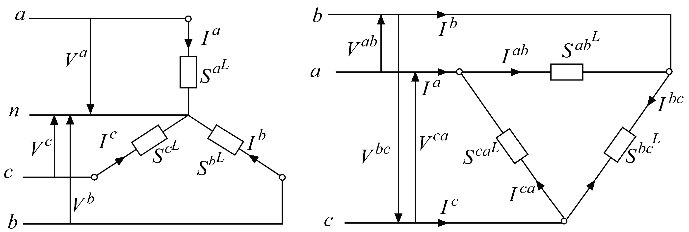
Three-phase loads can be connected in a grounded Wye (Y) configuration or an ungrounded delta ($\Delta$) configuration as shown in Figure 1. Loads are connected phase-to-neutral or phase-to-phase in a four-wire Wye configuration. Similarly, loads are connected phase-to-phase in a three-wire delta configuration.

Let us assume that ${\left(P_i^p\right)}^L$ and ${(Q_i^p)}^L$ are the active and reactive power loads, respectively, at bus i for a given phase p and modeled as the exponential load model described in Section 2.1. Then, in the case the Y connection is applied, three-phase loads and currents are given as follows:

$$\begin{array}{c}\hfill \left[\begin{array}{c}{(S_i^a)}^L\\ {(S_i^b)}^L\\ {(S_i^c)}^L\end{array}\right]=\left[\begin{array}{c}{(P_i^a)}^L+ı{(Q_i^a)}^L\\ {(P_i^b)}^L+ı{(Q_i^b)}^L\\ {(P_i^c)}^L+ı{(Q_i^c)}^L\end{array}\right]=\left[\begin{array}{c}\left({(P_{i0}^a)}^L+ı{(Q_{i0}^a)}^L\right){\left(\frac{|V_i^a|}{|V_0^a|}\right)}^n\\ \left({(P_{i0}^b)}^L+ı{(Q_{i0}^b)}^L\right){\left(\frac{|V_i^b|}{|V_0^b|}\right)}^n\\ \left({(P_{i0}^c)}^L+ı{(Q_{i0}^c)}^L\right){\left(\frac{|V_i^c|}{|V_0^c|}\right)}^n\end{array}\right],\left[\begin{array}{c}{I}_i^a\\ I_i^b\\ I_i^c\end{array}\right]=\left[\begin{array}{c}{\left(\frac{{(S_i^a)}^L}{V_i^a}\right)}^{*}\\ {\left(\frac{{(S_i^b)}^L}{V_i^b}\right)}^{*}\\ {\left(\frac{{(S_i^c)}^L}{V_i^c}\right)}^{*}\end{array}\right].\end{array}$$

(1)

In the case that the $\Delta$ connection is considered, three-phase loads and currents are given as follows:

$$\begin{array}{c}\hfill \left[\begin{array}{c}{(S_i^{ab})}^L\\ {(S_i^{bc})}^L\\ {(S_i^{ca})}^L\end{array}\right]=\left[\begin{array}{c}\left({(P_{i0}^{ab})}^L+ı{(Q_{i0}^{ab})}^L\right){\left(\frac{|V_i^{ab}|}{|V_0^{ab}|}\right)}^n\\ \left({(P_{i0}^{bc})}^L+ı{(Q_{i0}^{bc})}^L\right){\left(\frac{|V_i^{bc}|}{|V_0^{bc}|}\right)}^n\\ \left({(P_{i0}^{ca})}^L+ı{(Q_{i0}^{ca})}^L\right){\left(\frac{|V_i^{ca}|}{|V_0^{ca}|}\right)}^n\end{array}\right],\left[\begin{array}{c}{I}_i^a\\ I_i^b\\ I_i^c\end{array}\right]=\left[\begin{array}{c}{\left(\frac{{(S_i^{ab})}^L}{V_i^{ab}}\right)}^{*}-{\left(\frac{{(S_i^{ca})}^L}{V_i^{ca}}\right)}^{*}\\ {\left(\frac{{(S_i^{bc})}^L}{V_i^{bc}}\right)}^{*}-{\left(\frac{{(S_i^{ab})}^L}{V_i^{ab}}\right)}^{*}\\ {\left(\frac{{(S_i^{ca})}^L}{V_i^{ca}}\right)}^{*}-{\left(\frac{{(S_i^{bc})}^L}{V_i^{bc}}\right)}^{*}\end{array}\right].\end{array}$$

(2)

2.3. Generator Model

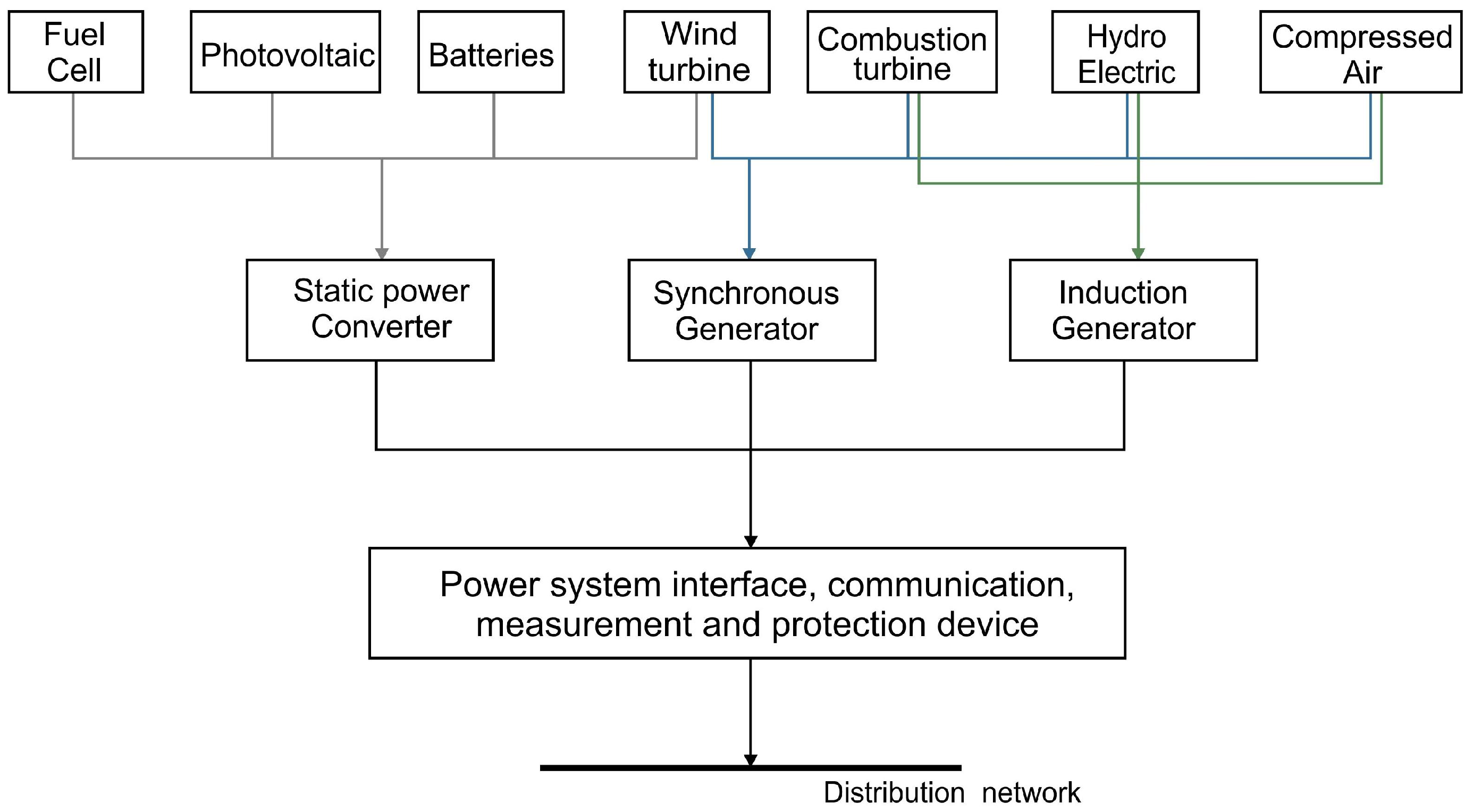
Since conventional power plants have controls for the active power P and the voltage magnitude $|V|$, they are modeled as a PV bus in the power flow analysis. However, most of the DGs do not have both P and $|V|$ controls and therefore they cannot be modeled as a PV bus. Figure 2 shows which type of power converter is employed to which types of renewable energy sources (DGs).

Depending on the types of energy sources and energy converters, the DGs are modeled as follows:

• The constant power factor model (PQ bus):
  The active power P output and power factor $pf$ are specified and the reactive power Q is determined by these two variables.
• The variable reactive power model (PQ bus):
  The active power P output is specified and the reactive power Q is determined by applying a predetermined polynomial function.
• The constant voltage model (PV bus):
  The active power P output and voltage magnitude $|V|$ are specified.

The DGs modeled as PQ buses can be treated as negative PQ loads in power flow analysis.

2.4. Transformer Model

Three-phase transformers are modeled by an admittance matrix $Y_T^{abc}$ which depends upon the connection of the primary and secondary taps, and the leakage admittance.

$$Y_T^{abc}=\left[\begin{array}{cc}{Y}_{pp}^{abc}& Y_{ps}^{abc}\\ Y_{sp}^{abc}& Y_{ss}^{abc}\end{array}\right]$$

(3)

where $Y_{ps}^{abc}$, $Y_{sp}^{abc}$ are a mutual admittance and $Y_{pp}^{abc}$, $Y_{ss}^{abc}$ are a self admittance of the primary and the secondary taps, respectively. The submatrices of the admittance matrix for different transformer connections are given in

Table 2. Characteristic submatrices of admittance matrices for different transformer connections.

Transformer Connection		Self Admittance		Mutual Admittance
Bus $\mathit{P}$	Bus $\mathit{S}$	${\mathit{Y}}_{\mathit{pp}}^{\mathit{abc}}$	${\mathit{Y}}_{\mathit{ss}}^{\mathit{abc}}$	${\mathit{Y}}_{\mathit{ps}}^{\mathit{abc}}$	${\mathit{Y}}_{\mathit{sp}}^{\mathit{abc}}$
Wye-G	Wye-G	$Y_I$	$Y_I$	$-Y_I$	$-Y_I$
Wye-G	Wye	$Y_{II}$	$Y_{II}$	$-Y_{II}$	$-Y_{II}$
Wye-G	Delta	$Y_I$	$Y_{II}$	$Y_{III}$	$Y_{III}^T$
Wye	Wye-G	$Y_{II}$	$Y_{II}$	$-Y_{II}$	$-Y_{II}$
Wye	Wye	$Y_{II}$	$Y_{II}$	$-Y_{II}$	$-Y_{II}$
Wye	Delta	$Y_{II}$	$Y_{II}$	$Y_{III}$	$Y_{III}^T$
Delta	Wye-G	$Y_{II}$	$Y_I$	$Y_{III}^T$	$Y_{III}$
Delta	Wye	$Y_{II}$	$Y_{II}$	$Y_{III}^T$	$Y_{III}$
Delta	Delta	$Y_{II}$	$Y_{II}$	$-Y_{II}$	$-Y_{II}$

.

In this table, submatrices are given as:

$$\begin{array}{c}\hfill Y_I=\left[\begin{array}{ccc}{y}_t& 0& 0\\ 0& y_t& 0\\ 0& 0& y_t\end{array}\right],Y_{II}=\frac{1}{3}\left[\begin{array}{ccc}2y_t& -y_t& -y_t\\ -y_t& 2y_t& -y_t\\ -y_t& -y_t& 2y_t\end{array}\right],Y_{III}=\frac{1}{\sqrt{3}}\left[\begin{array}{ccc}-y_t& y_t& 0\\ 0& -y_t& y_t\\ y_t& 0& -y_t\end{array}\right]\end{array}$$

(4)

and $y_t$ is the leakage admittance of the transformer. If the transformer has an off-nominal tap ratio $\alpha$:$\beta$ where $\alpha$ and $\beta$ are tappings on the primary and secondary sides respectively, then the submatrices must be modified as follows:

• Divide the self admittance matrix of the primary by ${\alpha }^2$: $\frac{Y_{pp}^{abc}}{{\alpha }^2}$
• Divide the self admittance matrix of the secondary by ${\beta }^2$: $\frac{Y_{ss}^{abc}}{{\beta }^2}$
• Divide the mutual admittance matrices by $\alpha \beta$: $\frac{Y_{ps}^{abc}}{\alpha \beta }$, $\frac{Y_{sp}^{abc}}{\alpha \beta }$

The admittance matrix (3) for the transformer can be added to the general admittance matrix in (5). For more detailed information, we refer to [15].

3. Power Flow Problem

The power flow, or load flow problem is the problem of computing the voltage magnitude $|V_i|$ and angle ${\delta }_i$ in each bus of a power system where the power generation and consumption are given. According to Kirchoff’s Current Law (KCL), the relation between the injected current I and the bus voltages V, is described by the admittance matrix $\mathbf{Y}$:

$$I=\mathbf{Y}V\leftrightarrow \left[\begin{array}{c}{I}_1^{abc}\\ ⋮\\ I_N^{abc}\end{array}\right]=\left[\begin{array}{ccc}{Y}_{11}^{abc}& \cdots & Y_{1N}^{abc}\\ ⋮& \ddots & ⋮\\ Y_{N1}^{abc}& \cdots & Y_{NN}^{abc}\end{array}\right]\left[\begin{array}{c}{V}_1^{abc}\\ ⋮\\ V_N^{abc}\end{array}\right].$$

(5)

In Equation (5), $I_i^{abc}$, $V_j^{abc},$ and $Y_{ij}^{abc}$ are given as:

$$\begin{array}{c}\hfill I_i^{abc}=\left[\begin{array}{c}{I}_i^a\\ I_i^b\\ I_i^c\end{array}\right],V_j^{abc}=\left[\begin{array}{c}{V}_j^a\\ V_j^b\\ V_j^c\end{array}\right],Y_{ij}^{abc}=\left[\begin{array}{ccc}{Y}_{ij}^{aa}& Y_{ij}^{ab}& Y_{ij}^{ac}\\ Y_{ij}^{ba}& Y_{ij}^{bb}& Y_{ij}^{bc}\\ Y_{ij}^{ca}& Y_{ij}^{cb}& Y_{ij}^{cc}\end{array}\right]\end{array}$$

(6)

where $I_i^p$ is the injected current, $V_i^p$ is the complex voltage at bus i for a given phase p, and $Y_{ij}^{pq}$ is the element of the admittance matrix. The injected current $I_i^p$ at bus i for a given phase p can be computed from Equation (5) as follows:

$$I_i^p=\sum _{k=1}^N\sum _{q=a,b,c}{Y}_{ik}^{pq}{V}_k^q.$$

(7)

The mathematical equations for the three-phase power flow problem are given by:

$$S_i^p=V_i^p{(I_i^p)}^{*}=V_i^p\sum _{k=1}^N\sum _{q=a,b,c}{(Y_{ik}^{pq})}^{*}{(V_k^q)}^{*}$$

(8)

where $S_i^p$ is the injected complex power. Mathematically, the power flow problem is a nonlinear system of equations.

4. Newton Power Flow Solution Methods

The Newton based power flow methods use the Newton–Raphson method which is used to solve a nonlinear system of equations $F(\overrightarrow{x})=0$. The linearized problem is constructed as the Jacobian matrix equation

$$-J(\overrightarrow{x})\Delta \overrightarrow{x}=F(\overrightarrow{x})$$

(9)

where $J(\overrightarrow{x})$ is the square Jacobian matrix and $\Delta \overrightarrow{x}$ is the correction vector. The Jacobian matrix is obtained by $J_{ik}=\frac{\partial F_i(\overrightarrow{x})}{\partial x_k}$ and is highly sparse in power flow applications [8,62]. Newton power flow methods (NRs) formulate $F(\overrightarrow{x})$ as power or current-mismatch functions and designate the unknown bus voltages as the problem variables $\overrightarrow{x}$.

4.1. The Power Mismatch Function

The power flow problem (8) is formulated as the power mismatch function $F(\overrightarrow{x})$ as follows:

$$\begin{array}{cc}\hfill F_i(\overrightarrow{x})=\Delta S_i^p& ={(S_i^p)}^{sp}-V_i^p\sum _{k=1}^N\sum _{q=a,b,c}{(Y_{ik}^{pq})}^{*}{(V_k^q)}^{*}\hfill \end{array}$$

(10)

where ${(S_i^p)}^{sp}$ is the specified complex power at bus i for a given phase p. In general, the specified complex power ${(S_i^p)}^{sp}$ injection at bus i is given by following equation:

$$\begin{array}{c}\hfill {(S_i^p)}^{sp}={(S_i^p)}^G-{(S_i^p)}^L\end{array}$$

where ${(S_i^p)}^G$ is the specified complex power generation, whereas ${(S_i^p)}^L={(P_i^p)}^L+ı{(Q_i^p)}^L$ is specified complex power load at bus i for a given phase p. Here, ${(P_i^p)}^L$ and ${(Q_i^p)}^L$ can be modeled as one of the load models described in Section 2.1.

4.2. The Current Mismatch Function

The power flow problem (8) is formulated as the current-mismatch function $F(\overrightarrow{x})$ as follows:

$$\begin{array}{cc}\hfill F_i(\overrightarrow{x})=\Delta I_i^p& ={\left(\frac{{(S_i^p)}^{sp}}{V_i^p}\right)}^{*}-\sum _{k=1}^N\sum _{q=a,b,c}{Y}_{ik}^{pq}{V}_k^q\hfill \end{array}$$

(11)

where ${(S_i^p)}^{sp}$ is the specified complex power at bus i for a given phase p.

The power mismatch (10) and current mismatch (11) functions given in complex form can be reformulated into real equations and variables using polar and Cartesian coordinates. These two mismatch functions (power and current) and three coordinates (polar, Cartesian and complex form), result in six versions of the Newton–Raphson method for the solution of power flow problems. The detailed explanations of all six versions can be found in [65]. Only the version using the current mismatch functions in polar coordinates is explained in the following section. The remaining versions can be derived similarly.

4.2.1. Polar Current Mismatch Version (NR-c-pol)

In this version, the current mismatch function (11) is rewritten for real and imaginary parts using polar coordinates as follows:

$$\begin{array}{cc}\hfill \Delta {(I_i^r)}^p(\overrightarrow{x})& =\frac{{(P_i^{sp})}^p\cos {\delta }_i^p+{(Q_i^{sp})}^p\sin {\delta }_i^p}{|V_i^p|}-\sum _{k=1}^N\sum _{q=a,b,c}|V_k^q|(G_{ik}^{pq}\cos {\delta }_k^q-B_{ik}^{pq}\sin {\delta }_k^q)\hfill \end{array}$$

(12)

$$\begin{array}{cc}\hfill \Delta {(I_i^m)}^p(\overrightarrow{x})& =\frac{{(P_i^{sp})}^p\sin {\delta }_i^p-{(Q_i^{sp})}^p\cos {\delta }_i^p}{|V_i^p|}-\sum _{k=1}^N\sum _{q=a,b,c}|V_k^q|(G_{ik}^{pq}\sin {\delta }_k^q+B_{ik}^{pq}\cos {\delta }_k^q).\hfill \end{array}$$

(13)

The current mismatch function can be written in vector form as follows:

$$F(\overrightarrow{x})=\left[\begin{array}{c}\Delta {(I_1^r)}^{abc}\\ ⋮\\ \Delta {(I_N^r)}^{abc}\\ \Delta {(I_1^m)}^{abc}\\ ⋮\\ \Delta {(I_N^m)}^{abc}\end{array}\right]$$

(14)

where

$$\begin{array}{c}\hfill \Delta {(I_i^r)}^{abc}=\left[\begin{array}{c}\Delta {(I_i^r)}^a(\overrightarrow{x})\\ \Delta {(I_i^r)}^b(\overrightarrow{x})\\ \Delta {(I_i^r)}^c(\overrightarrow{x})\end{array}\right],\Delta {(I_i^m)}^{abc}=\left[\begin{array}{c}\Delta {(I_i^m)}^a(\overrightarrow{x})\\ \Delta {(I_i^m)}^b(\overrightarrow{x})\\ \Delta {(I_i^m)}^c(\overrightarrow{x})\end{array}\right]\end{array}$$

(15)

and we look for the solution where the current mismatch function (14) is equal to zero:

$$F(\overrightarrow{x})=0.$$

(16)

Application of a first-order Taylor approximation to the current mismatch function (14) results in a linear system of equations that is solved in every Newton iteration:

$$J(\overrightarrow{x})\Delta \overrightarrow{x}=F(\overrightarrow{x})$$

(17)

where $\Delta \overrightarrow{x}$ is the correction and $J(\overrightarrow{x})$ is the Jacobian matrix of the current mismatch function. Here, the Jacobian matrix is obtained by taking all first-order partial derivatives of the current mismatch function with respect to the voltage angles ${\delta }^p$ and magnitudes ${|V|}^p$ as: if $i\ne k$

$$\begin{array}{cc}\hfill \frac{\partial \Delta {(I_i^r)}^p(\overrightarrow{x})}{\partial |V_k^p|}& =-(G_{ik}^{pp}\cos {\delta }_k^p-B_{ik}^{pp}\sin {\delta }_k^p)\hfill \\ \hfill \frac{\partial \Delta {(I_i^r)}^p(\overrightarrow{x})}{\partial {\delta }_k^p}& =|V_k^p|(G_{ik}^{pp}\sin {\delta }_k^p+B_{ik}^{pp}\cos {\delta }_k^p)\hfill \\ \hfill \frac{\partial \Delta {(I_i^m)}^p(\overrightarrow{x})}{\partial |V_k^p|}& =-(G_{ik}^{pp}\sin {\delta }_k^p+B_{ik}^{pp}\cos {\delta }_k^p)\hfill \\ \hfill \frac{\partial \Delta {(I_i^m)}^p(\overrightarrow{x})}{\partial {\delta }_k^p}& =-|V_k^p|(G_{ik}^{pp}\cos {\delta }_k^p-B_{ik}^{pp}\sin {\delta }_k^p)\hfill \end{array}$$

if $i=k$

$$\begin{array}{cc}\hfill \frac{\partial \Delta {(I_i^r)}^p(\overrightarrow{x})}{\partial |V_i^p|}& =-(G_{ii}^{pp}\cos {\delta }_i^p-B_{ii}^{pp}\sin {\delta }_i^p)-\frac{{(P_i^{sp})}^p\cos {\delta }_i^p+{(Q_i^{sp})}^p\sin {\delta }_i^p}{|V_i^p{|}^2}\hfill \\ \hfill \frac{\partial \Delta {(I_i^r)}^p(\overrightarrow{x})}{\partial {\delta }_i^p}& =|V_i^p|(G_{ii}^{pp}\sin {\delta }_i^p+B_{ii}^{pp}\cos {\delta }_i^p)-\frac{{(P_i^{sp})}^p\sin {\delta }_i^p-{(Q_i^{sp})}^p\cos {\delta }_i^p}{|V_i^p|}\hfill \\ \hfill \frac{\partial \Delta {(I_i^m)}^p(\overrightarrow{x})}{\partial |V_i^p|}& =-(G_{ii}^{pp}\sin {\delta }_i^p+B_{ii}^{pp}\cos {\delta }_i^p)-\frac{{(P_i^{sp})}^p\sin {\delta }_i^p-{(Q_i^{sp})}^p\cos {\delta }_i^p}{|V_i^p{|}^2}\hfill \\ \hfill \frac{\partial \Delta {(I_i^m)}^p(\overrightarrow{x})}{\partial {\delta }_i^p}& =-|V_i^p|(G_{ii}^{pp}\cos {\delta }_i^p-B_{ii}^{pp}\sin {\delta }_i^p)+\frac{{(P_i^{sp})}^p\cos {\delta }_i^p+{(Q_i^{sp})}^p\sin {\delta }_i^p}{|V_i^p|}\hfill \end{array}$$

The linear system of Equation (17) that is solved in every Newton iteration can be written in matrix form as follows:

$$-\left[\begin{array}{cccccc}\frac{\partial \Delta {(I_1^r)}^{abc}}{\partial {\delta }_1^{abc}}& \cdots & \frac{\partial \Delta {(I_1^r)}^{abc}}{\partial {\delta }_N^{abc}}& \frac{\partial \Delta {(I_1^r)}^{abc}}{\partial |V_1^{abc}|}& \cdots & \frac{\partial \Delta {(I_1^r)}^{abc}}{\partial |V_N^{abc}|}\\ ⋮& \ddots & ⋮& ⋮& \ddots & ⋮\\ \frac{\partial \Delta {(I_N^r)}^{abc}}{\partial {\delta }_1^{abc}}& \cdots & \frac{\partial \Delta {(I_N^r)}^{abc}}{\partial {\delta }_N^{abc}}& \frac{\partial \Delta {(I_N^r)}^{abc}}{\partial |V_1^{abc}|}& \cdots & \frac{\partial \Delta {(I_N^r)}^{abc}}{\partial |V_N^{abc}|}\\ \frac{\partial \Delta {(I_1^m)}^{abc}}{\partial {\delta }_1^{abc}}& \cdots & \frac{\partial \Delta {(I_1^m)}^{abc}}{\partial {\delta }_N^{abc}}& \frac{\partial \Delta {(I_1^m)}^{abc}}{\partial |V_1^{abc}|}& \cdots & \frac{\partial \Delta {(I_1^m)}^{abc}}{\partial |V_N^{abc}|}\\ ⋮& \ddots & ⋮& ⋮& \ddots & ⋮\\ \frac{\partial \Delta {(I_N^m)}^{abc}}{\partial {\delta }_1^{abc}}& \cdots & \frac{\partial \Delta {(I_N^m)}^{abc}}{\partial {\delta }_N^{abc}}& \frac{\partial \Delta {(I_N^m)}^{abc}}{\partial |V_1^{abc}|}& \cdots & \frac{\partial \Delta {(I_N^m)}^{abc}}{\partial |V_N^{abc}|}\end{array}\right]\left[\begin{array}{c}\Delta {\delta }_1^{abc}\\ ⋮\\ \frac{\Delta {\delta }_N^{abc}}{\Delta |V_1^{abc}|}\\ ⋮\\ \Delta |V_N^{abc}|\end{array}\right]=\left[\begin{array}{c}\Delta {(I_1^r)}^{abc}\\ ⋮\\ \frac{\Delta {(I_N^r)}^{abc}}{\Delta {(I_1^m)}^{abc}}\\ ⋮\\ \Delta {(I_N^m)}^{abc}\end{array}\right]$$

(18)

where

$$\begin{array}{cc}\hfill \Delta {\delta }_i^{abc}& =\left[\begin{array}{c}\Delta {\delta }_i^a\\ \Delta {\delta }_i^b\\ \Delta {\delta }_i^c\end{array}\right],\frac{\partial \Delta {(I_i^r)}^{abc}}{\partial {\delta }_j^{abc}}=\left[\begin{array}{ccc}\frac{\partial \Delta {(I_i^r)}^a}{\partial {\delta }_j^a}& \frac{\partial \Delta {(I_i^r)}^a}{\partial {\delta }_j^b}& \frac{\partial \Delta {(I_i^r)}^a}{\partial {\delta }_j^c}\\ \frac{\partial \Delta {(I_i^r)}^b}{\partial {\delta }_j^a}& \frac{\partial \Delta {(I_i^r)}^b}{\partial {\delta }_j^b}& \frac{\partial \Delta {(I_i^r)}^b}{\partial {\delta }_j^c}\\ \frac{\partial \Delta {(I_i^r)}^c}{\partial {\delta }_j^a}& \frac{\partial \Delta {(I_i^r)}^c}{\partial {\delta }_j^b}& \frac{\partial \Delta {(I_i^r)}^c}{\partial {\delta }_j^c}\end{array}\right],\hfill \end{array}$$

(19)

$$\begin{array}{cc}\hfill \Delta |V_i^{abc}|& =\left[\begin{array}{c}\Delta |V_i^a|\\ \Delta |V_i^b|\\ \Delta |V_i^c|\end{array}\right],\frac{\partial \Delta {(I_i^m)}^{abc}}{\partial |V_j^{abc}|}=\left[\begin{array}{ccc}\frac{\partial \Delta {(I_i^m)}^a}{\partial |V_j^a|}& \frac{\partial \Delta {(I_i^m)}^a}{\partial |V_j^b|}& \frac{\partial \Delta {(I_i^m)}^a}{\partial |V_j^c|}\\ \frac{\partial \Delta {(I_i^m)}^b}{\partial |V_j^a|}& \frac{\partial \Delta {(I_i^m)}^b}{\partial |V_j^b|}& \frac{\partial \Delta {(I_i^m)}^b}{\partial |V_j^c|}\\ \frac{\partial \Delta {(I_i^m)}^c}{\partial |V_j^a|}& \frac{\partial \Delta {(I_i^m)}^c}{\partial |V_j^b|}& \frac{\partial \Delta {(I_i^m)}^c}{\partial |V_j^c|}\end{array}\right].\hfill \end{array}$$

(20)

The bus voltage correction in polar coordinate is given by:

$$\begin{array}{ccc}\hfill {|V_i^p|}^{(h+1)}& =& {|V_i^p|}^{(h)}+\Delta {|V_i^p|}^{(h)}\hfill \end{array}$$

(21)

$$\begin{array}{ccc}\hfill {({\delta }_i^p)}^{(h+1)}& =& {({\delta }_i^p)}^{(h)}+\Delta {({\delta }_i^p)}^{(h)}\hfill \end{array}$$

(22)

where h is the iteration counter. Then the complex voltage at bus i can be computed by:

$${(V_i^p)}^{(h+1)}={|V_i^p|}^{(h+1)}{e}^{ı{({\delta }_i^p)}^{(h+1)}}.$$

(23)

4.2.2. Representation of PV Buses for NR-c-pol

In case of a PV bus j, a voltage magnitude $|V_j^{abc}|$ is specified instead of reactive power $Q_j^{abc}$ where

$$\begin{array}{c}\hfill |V_j^{abc}|=\left[\begin{array}{c}|V_j^a|\\ |V_j^b|\\ |V_j^c|\end{array}\right],Q_j^{abc}=\left[\begin{array}{c}{Q}_j^a\\ Q_j^b\\ Q_j^c\end{array}\right].\end{array}$$

(24)

In the current mismatch formulation, it is possible to choose the reactive power $Q_j^p$ at the bus j for a given phase p as an unknown variable as a voltage magnitude $|V|$ or an angle $\delta$. Since $Q_j^{abc}$ is an unknown variable, all the first-order partial derivatives $\frac{\partial \Delta {(I_i^r)}^{abc}}{\partial Q_j^{abc}}$ and $\frac{\partial {(\Delta I_i^m)}^{abc}}{\partial Q_j^{abc}}$ must be computed as:

$$\begin{array}{c}\hfill \frac{\partial \Delta {(I_i^r)}^{abc}}{\partial Q_j^{abc}}=\left[\begin{array}{ccc}\frac{\partial \Delta {(I_i^r)}^a}{\partial Q_j^a}& \frac{\partial \Delta {(I_i^r)}^a}{\partial Q_j^b}& \frac{\partial \Delta {(I_i^r)}^a}{\partial Q_j^c}\\ \frac{\partial \Delta {(I_i^r)}^b}{\partial Q_j^a}& \frac{\partial \Delta {(I_i^r)}^b}{\partial Q_j^b}& \frac{\partial \Delta {(I_i^r)}^b}{\partial Q_j^c}\\ \frac{\partial \Delta {(I_i^r)}^c}{\partial Q_j^a}& \frac{\partial \Delta {(I_i^r)}^c}{\partial Q_j^b}& \frac{\partial \Delta {(I_i^r)}^c}{\partial Q_j^c}\end{array}\right],\frac{\partial \Delta {(I_i^m)}^{abc}}{\partial Q_j^{abc}}=\left[\begin{array}{ccc}\frac{\partial \Delta {(I_i^m)}^a}{\partial Q_j^a}& \frac{\partial \Delta {(I_i^m)}^a}{\partial Q_j^b}& \frac{\partial \Delta {(I_i^m)}^a}{\partial Q_j^c}\\ \frac{\partial \Delta {(I_i^m)}^b}{\partial Q_j^a}& \frac{\partial \Delta {(I_i^m)}^b}{\partial Q_j^b}& \frac{\partial \Delta {(I_i^m)}^b}{\partial Q_j^c}\\ \frac{\partial \Delta {(I_i^m)}^c}{\partial Q_j^a}& \frac{\partial \Delta {(I_i^m)}^c}{\partial Q_j^b}& \frac{\partial \Delta {(I_i^m)}^c}{\partial Q_j^c}\end{array}\right]\end{array}$$

(25)

where if $i\ne j$

$$\begin{array}{c}\hfill \frac{\partial \Delta {(I_i^r)}^{abc}(\overrightarrow{x})}{\partial Q_j^{abc}}=\left[\begin{array}{ccc}0& 0& 0\\ 0& 0& 0\\ 0& 0& 0\end{array}\right],\frac{\partial \Delta {(I_i^m)}^{abc}(\overrightarrow{x})}{\partial Q_j^{abc}}=\left[\begin{array}{ccc}0& 0& 0\\ 0& 0& 0\\ 0& 0& 0\end{array}\right]\end{array}$$

(26)

if $i=j$

$$\begin{array}{c}\hfill \frac{\partial \Delta {(I_j^r)}^{abc}(\overrightarrow{x})}{\partial Q_j^{abc}}=\left[\begin{array}{ccc}\frac{\sin {\delta }_j^a}{|V_j^a{|}^{sp}}& 0& 0\\ 0& \frac{\sin {\delta }_j^b}{|V_j^b{|}^{sp}}& 0\\ 0& 0& \frac{\sin {\delta }_j^c}{|V_j^c{|}^{sp}}\end{array}\right],\frac{\partial \Delta {(I_j^r)}^{abc}(\overrightarrow{x})}{\partial Q_j^{abc}}=-\left[\begin{array}{ccc}\frac{\cos {\delta }_j^a}{|V_j^a{|}^{sp}}& 0& 0\\ 0& \frac{\cos {\delta }_j^b}{|V_j^b{|}^{sp}}& 0\\ 0& 0& \frac{\cos {\delta }_j^c}{|V_j^c{|}^{sp}}\end{array}\right]\end{array}$$

(27)

When the derivatives $\frac{\partial \Delta {(I_i^r)}^{abc}}{\partial Q_j^{abc}}$ and $\frac{\partial \Delta {(I_i^m)}^{abc}}{\partial Q_j^{abc}}$ are added into the Jacobian matrix $J(\overrightarrow{x})$, the Jacobian matrix becomes a rectangular matrix. However, all derivatives of real $\Delta {(I_i^r)}^{abc}$ and reactive $\Delta {(I_i^m)}^{abc}$ current mismatch functions with respect to $|V_j^{abc}|$ cannot be taken since $|V_j^{abc}|$ is not an unknown variable. Therefore, we can remove all the $\frac{\partial \Delta {(I_i^r)}^{abc}}{\partial |V_j^{abc}|}$ and $\frac{\partial \Delta {(I_i^m)}^{abc}}{\partial |V_j^{abc}|}$ from the Jacobian matrix $J(\overrightarrow{x})$ and the correction $\Delta |V_j^{abc}|$ can be replaced by $\Delta Q_j^{abc}$. Thus, the Jacobian matrix $J(\overrightarrow{x})$ is again square and therefore we will have a unique solution. The initial reactive power ${(Q_j^p)}^0$ at PV bus j for a given phase p is computed as follows:

$${(Q_j^p)}^0=\sum _{k=1}^N\sum _{q=a,b,c}|V_j^p||V_k^q|(G_{jk}^{pq}\sin {\delta }_{jk}^q-B_{jk}^{pq}\cos {\delta }_{jk}^q).$$

(28)

The reactive power is updated at each iteration use.

$$\begin{array}{ccc}\hfill {(Q_j^p)}^{(h+1)}& =& {(Q_j^p)}^{(h)}+\Delta {(Q_j^p)}^{(h)}.\hfill \end{array}$$

(29)

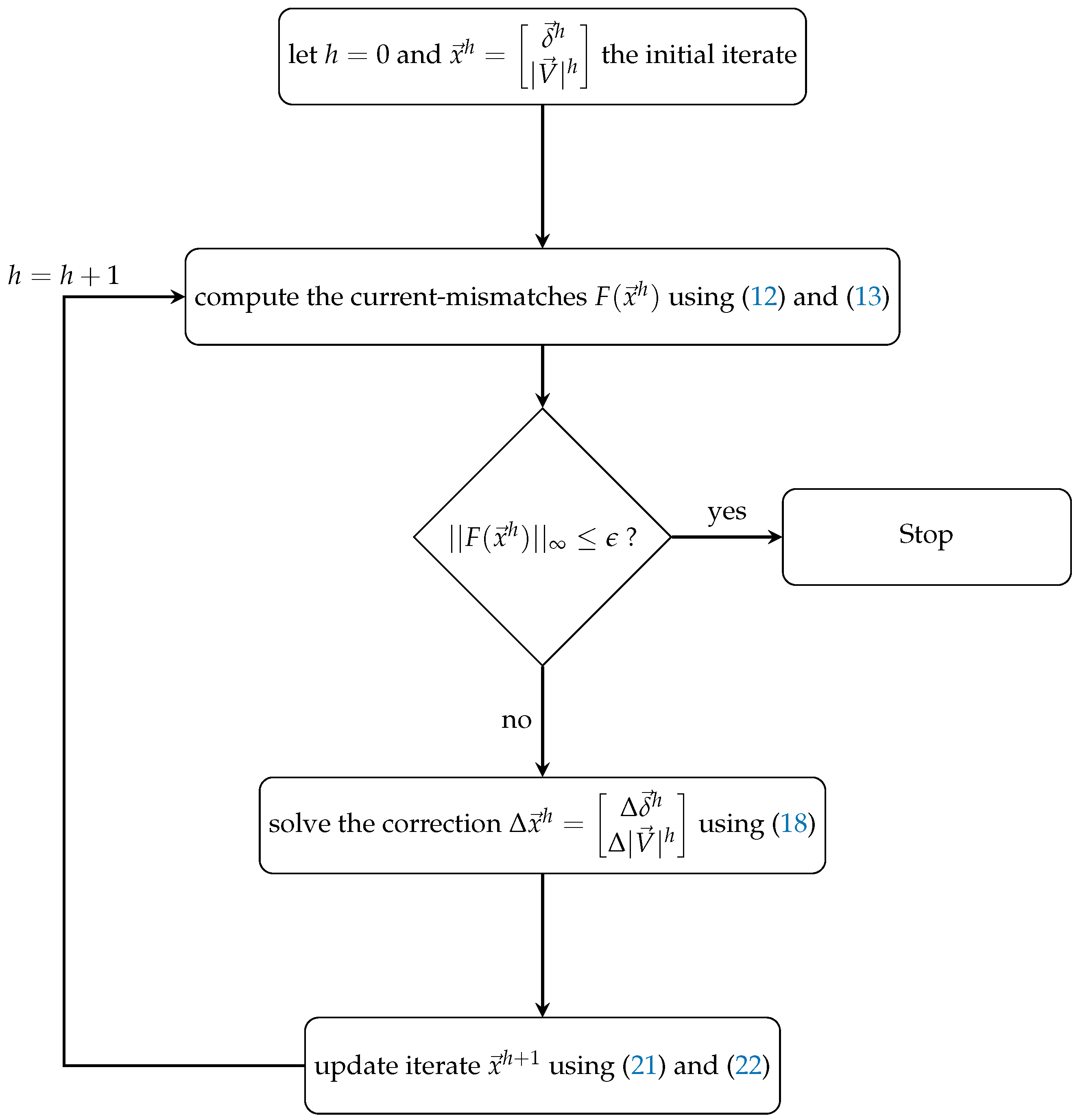
The flow chart of the polar current mismatch version (NR-c-pol) is given in Figure 3. The remaining versions of the Newton power flow method (NR) such as Cartesian current mismatch (NR-c-car), complex current mismatch (NR-c-com), Cartesian power mismatch (NR-p-car), and complex power mismatch (NR-p-com) which are newly developed for a single-phase power flow problem in [65], can be extended to a three-phase power flow problem analogously.

5. Numerical Experiment

We have shown how all versions of the Newton power flow method, originally developed for single-phase power flow problems in [65], can be extended to three-phase power flow problems with unbalanced distribution networks. Depending on the properties of a given network, one version can work better than the other versions. Therefore, it is crucial to study which version is more suitable for which kind of a power network. We use different load models, transformer connections, loading conditions, and $R/X$ ratios in order to analyze the convergence ability and scalability of all versions. Different loading conditions are considered by multiplying each bus’s power S by a constant k as $S=k*S$. Similarly, different $R/X$ ratios are obtained by multiplying each branch resistance by a constant k as $Z=k*R+ıX$. Finally, the performance of the solution methods is evaluated for constant power and constant polynomial load models as defined in Section 2.1. The most widely used version using power mismatch function in polar coordinates (NR-p-pol [8]) of the Newton power flow method and backward–forward sweep-based algorithm (BFS [43]) are applied for comparison purposes.

Two balanced distribution networks (33-bus [70] and 69-bus [71]) and two unbalanced distribution networks (IEEE 13-bus [72] and IEEE 37-bus [72]) are used for the numerical experiment. All methods are implemented in Matlab and the relative convergence tolerance $ϵ$ is set to ${10}^{-5}$. The maximum number of iterations is set to 50. Experiments are performed on an Intel computer i5-4690 3.5 GHz CPU with four cores and 64 Gb memory, running a Debian 64-bit Linux 8.7 distribution.

5.1. Single-Phase Problems

The convergence results of all solution methods for balanced distribution networks (DCase33 [70] and DCase69 [71]) are shown in

Table 3. Balanced distribution networks: DCase33 and DCase69.

Methods	Test Cases
	DCase33			DCase69
	Iter	Time	$||\mathit{F}(\overrightarrow{\mathit{x}}){||}_{\infty }$	Iter	Time	$||\mathit{F}(\overrightarrow{\mathit{x}}){||}_{\infty }$
NR-p-pol [8]	3	0.0123	$7.4675\times {10}^{-6}$	4	0.0131	$5.5875\times {10}^{-9}$
NR-p-car	3	0.0067	$1.0433\times {10}^{-6}$	3	0.0069	$8.1777\times {10}^{-6}$
NR-p-com	6	0.0058	$6.4610\times {10}^{-6}$	7	0.0060	$4.0138\times {10}^{-6}$
NR-c-pol	3	0.0087	$1.4291\times {10}^{-9}$	3	0.0090	$8.5226\times {10}^{-9}$
NR-c-car	3	0.0073	$1.3954\times {10}^{-9}$	3	0.0077	$1.9503\times {10}^{-8}$
NR-c-com	7	0.0068	$5.3792\times {10}^{-6}$	10	0.0084	$2.7697\times {10}^{-6}$
BFS [43]	7	0.0102	$1.0454\times {10}^{-6}$	7	0.0104	$7.7770\times {10}^{-6}$

.

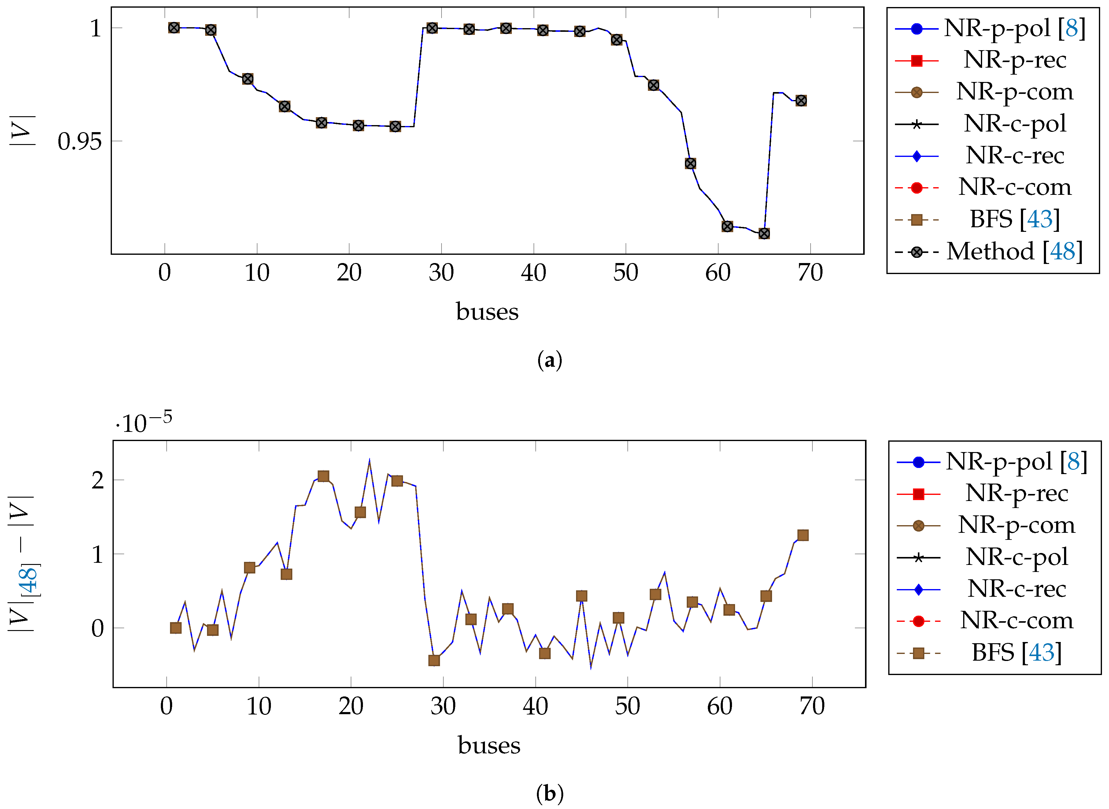
From Table 3, we see that NR-c-pol and NR-c-car versions have better performance in terms of a number of iterations and the norm of the residual of the mismatch function. Although NR-p-pol [8] and NR-p-car versions converged after the same number of iterations, the value of the residual norm is larger than for the NR-c-pol and NR-c-car versions. This means that if we set the tolerance to ${10}^{-7}$, these versions will need extra iterations to converge, whereas NR-c-pol and NR-c-car versions still converge after three iterations. We also see that NR-p-com, NR-c-com and BFS [43] methods need more iterations and have a linear convergence compared to other versions which have a quadratic convergence. These three methods solve the power flow problem in complex form, whereas other versions (NR-p-car, NR-p-pol, NR-c-car, and NR-c-pol) reformulate the problem into real equations using Cartesian and polar coordinates. Figure 4a shows the comparison of the results obtained by proposed solution methods with the well-known result of the existing method [48] for the computed voltage magnitude of DCase69. All the results of the proposed solution methods match the well-known result well with accuracy of ${10}^{-5}$ as shown in Figure 4b.

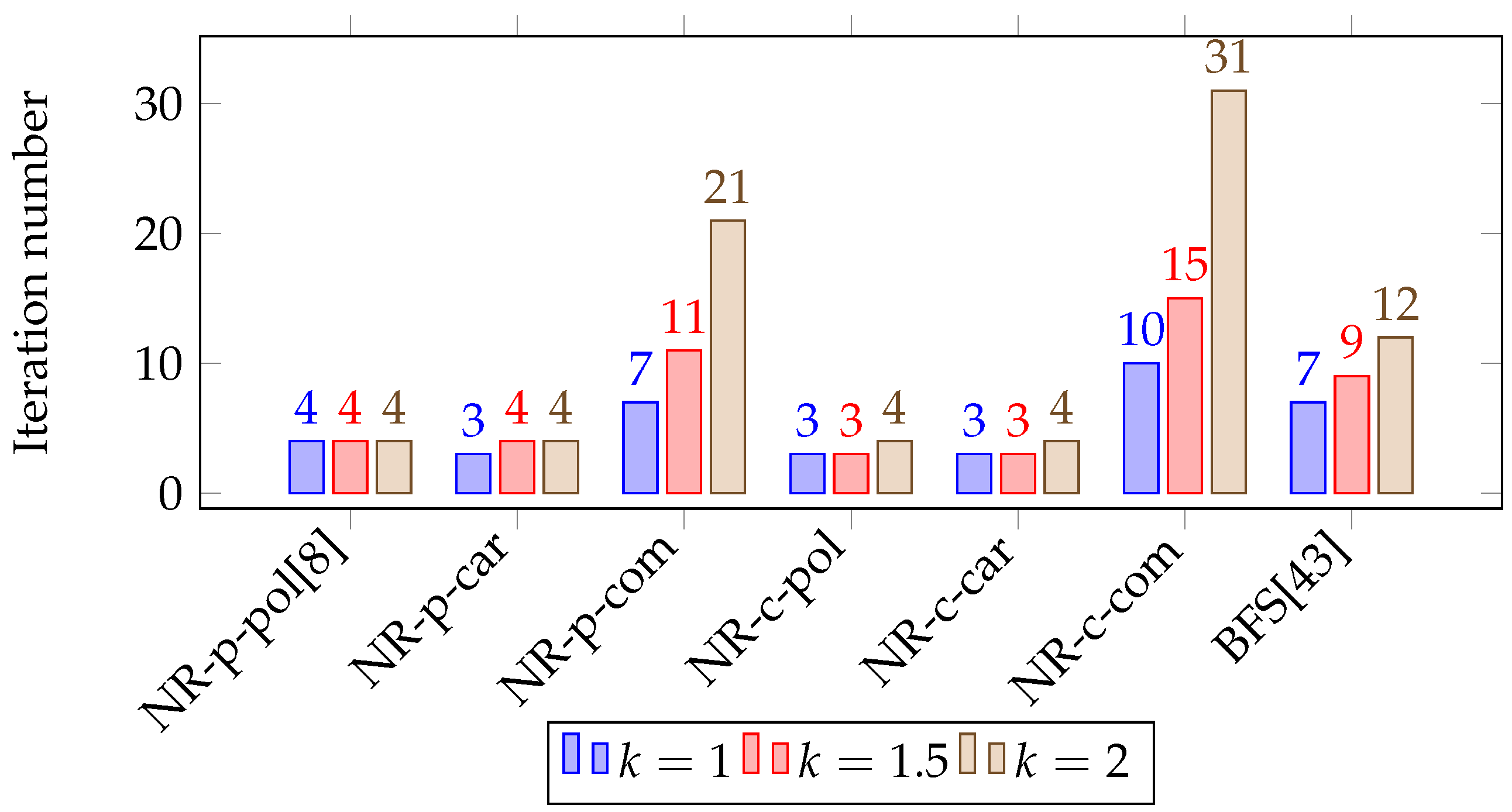
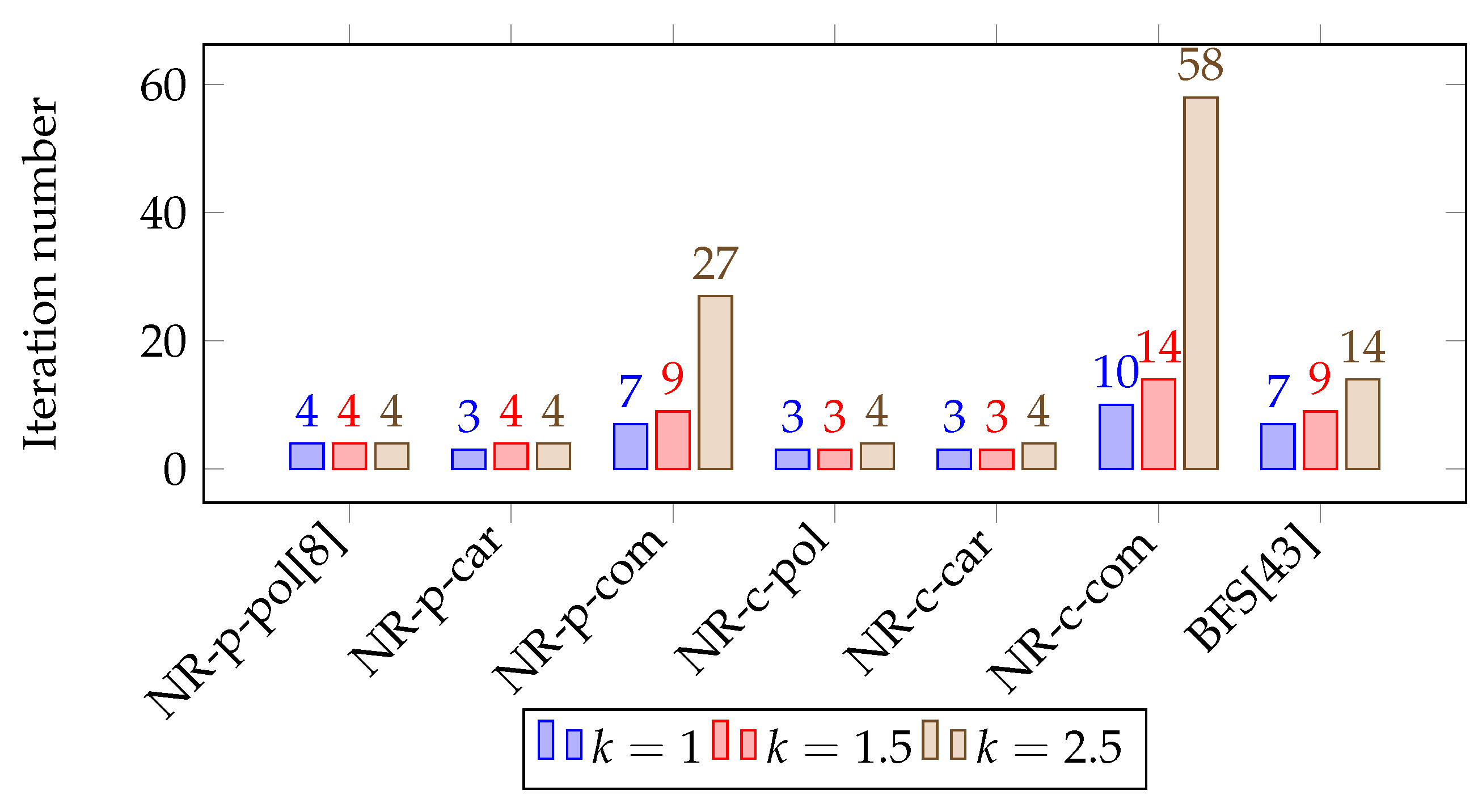
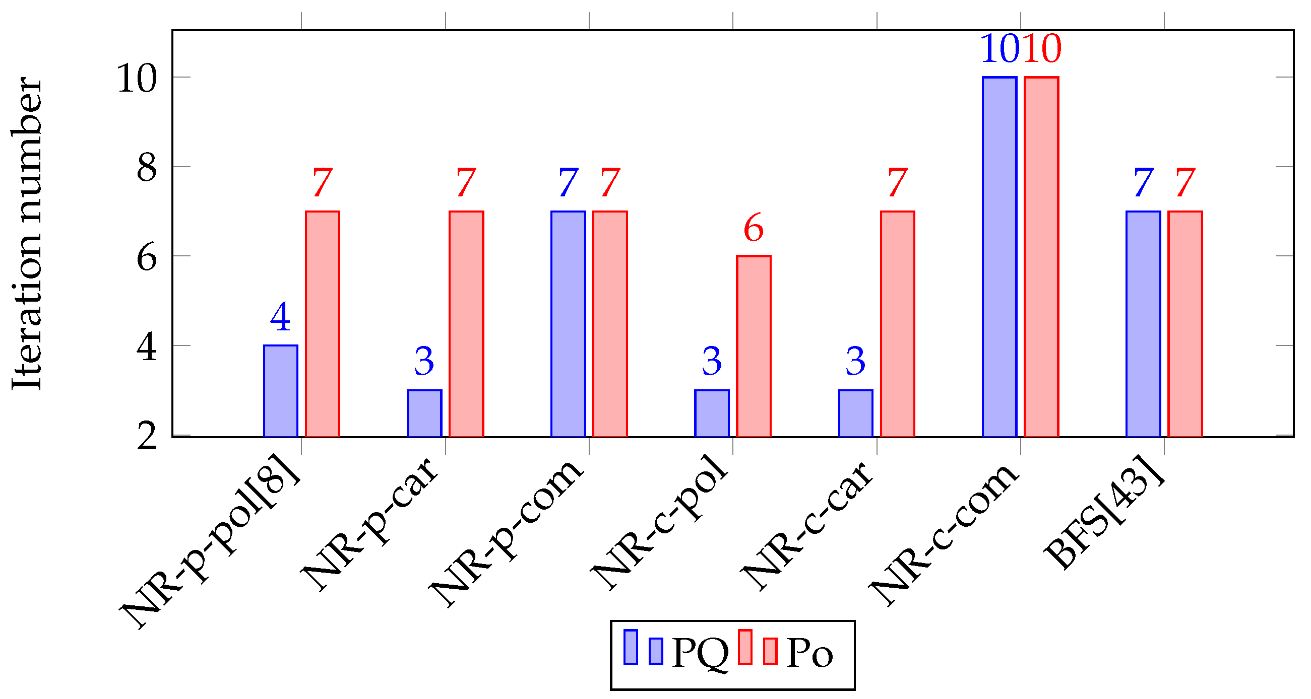
A convergence result of all solution methods for the balanced distribution network DCase69 with different loading conditions and different $R/X$ ratios, is shown in Figure 5 and Figure 6, respectively. We see that NR-p-com, NR-c-com, and BFS [43] are more sensitive to the change of loads and $R/X$ ratios compared to other versions that use real variables and values for the problem formulation using polar and Cartesian coordinates. Figure 7 shows the convergence of all solution methods for different load models. It is clear that for all methods, a constant power (PQ) model is more suitable to use on a balanced distribution network.

Thus, we can conclude that NR-c-pol and NR-c-car versions developed in [65] are more suitable for balanced distribution networks than versions using power mismatch functions (NR-p-pol [8], NR-p-car). Furthermore, NR-p-com and NR-c-com versions, as well as BFS [43] are the least preferable methods for balanced distribution networks in terms of convergence and robustness.

5.2. Three-Phase Problems

For IEEE 13-bus (DCase13) and IEEE 37-bus (DCase37) test networks, regulators are removed and all three-phase loads are chosen to be connected in a grounded Wye configuration as defined in Section 2.2. For the unbalanced distribution network DCase13, the transformer is connected in Wye-G, whereas DCase37 has the delta–delta transformer connection as defined in Section 2.4. The BFS method [43] is not implemented for three-phase power flow problems since it is not explained in sufficient detail how the three-phase transformer is handled for this method. The convergence result of all solution methods for unbalanced distribution networks (DCase13 and DCase37) is shown in

Table 4. Unbalanced distribution networks: DCase13 and DCase37.

Methods	Test Cases
	DCase13			DCase37
	Iter	Time	$||\mathit{F}(\overrightarrow{\mathit{x}}){||}_{\infty }$	Iter	Time	$||\mathit{F}(\overrightarrow{\mathit{x}}){||}_{\infty }$
NR-p-pol [8]	3	0.0116	$1.5571\times {10}^{-9}$	2	0.0134	$3.4150\times {10}^{-7}$
NR-p-car	3	0.0067	$6.7018\times {10}^{-9}$	2	0.0069	$1.1627\times {10}^{-7}$
NR-p-com	5	0.0055	$5.0957\times {10}^{-7}$	3	0.0055	$5.3394\times {10}^{-7}$
NR-c-pol	3	0.0087	$6.9974\times {10}^{-11}$	2	0.0094	$3.9750\times {10}^{-8}$
NR-c-car	3	0.0073	$8.1499\times {10}^{-11}$	2	0.0079	$4.0339\times {10}^{-8}$
NR-c-com	5	0.0067	$3.5585\times {10}^{-7}$	3	0.0065	$7.4985\times {10}^{-7}$

.

From Table 4, we see that except for the NR-p-com and NR-c-com versions, all methods converged after the same number of iterations for both unbalanced distribution networks. However, NR-c-pol and NR-c-car versions have better performance in terms of both number of iterations and residual norm of the mismatch function, as we had the same result for balanced distribution networks. Again, NR-p-com and NR-c-com versions need more iterations to converge compared to other versions.

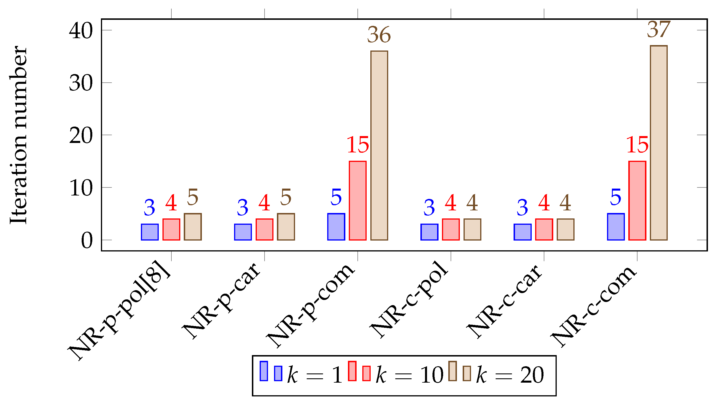
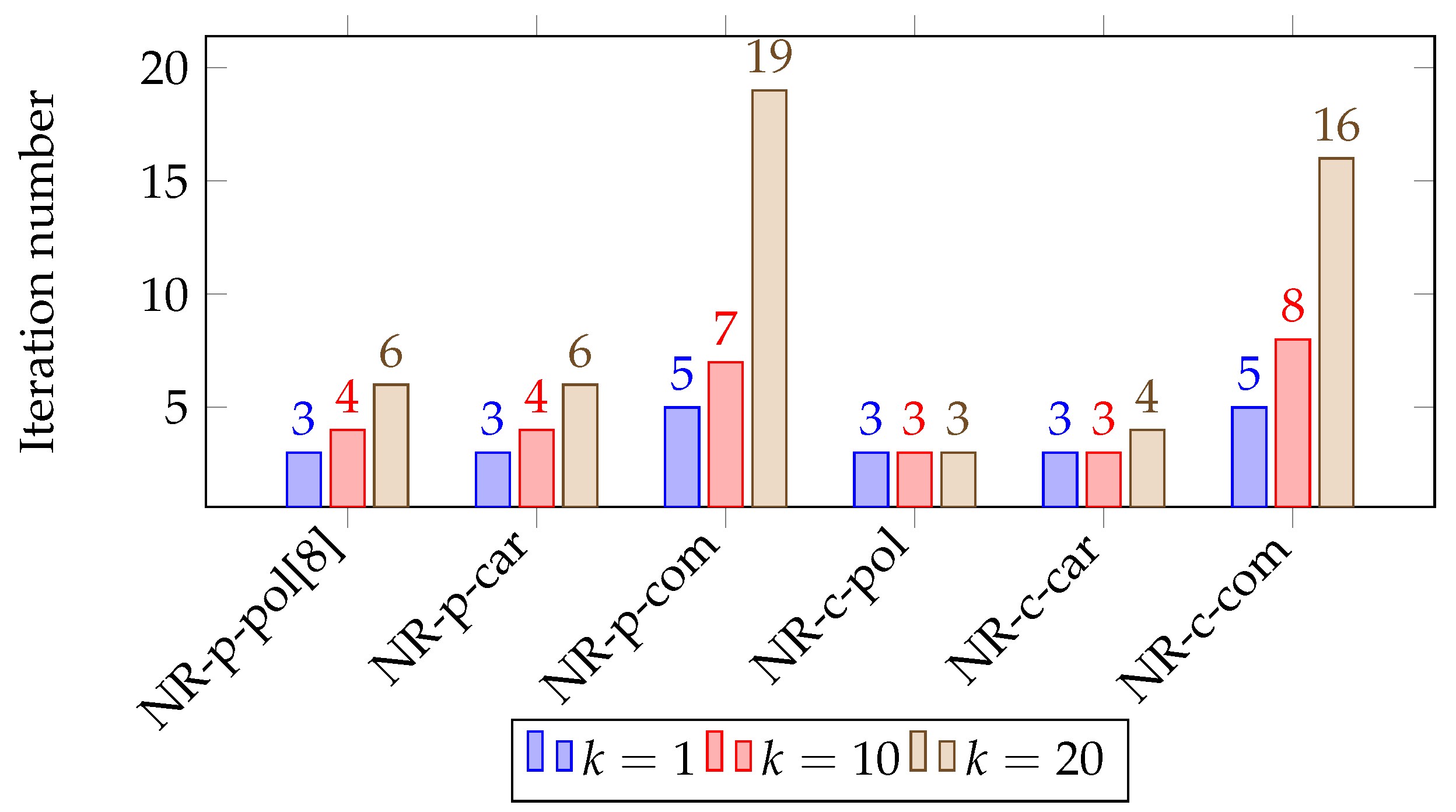
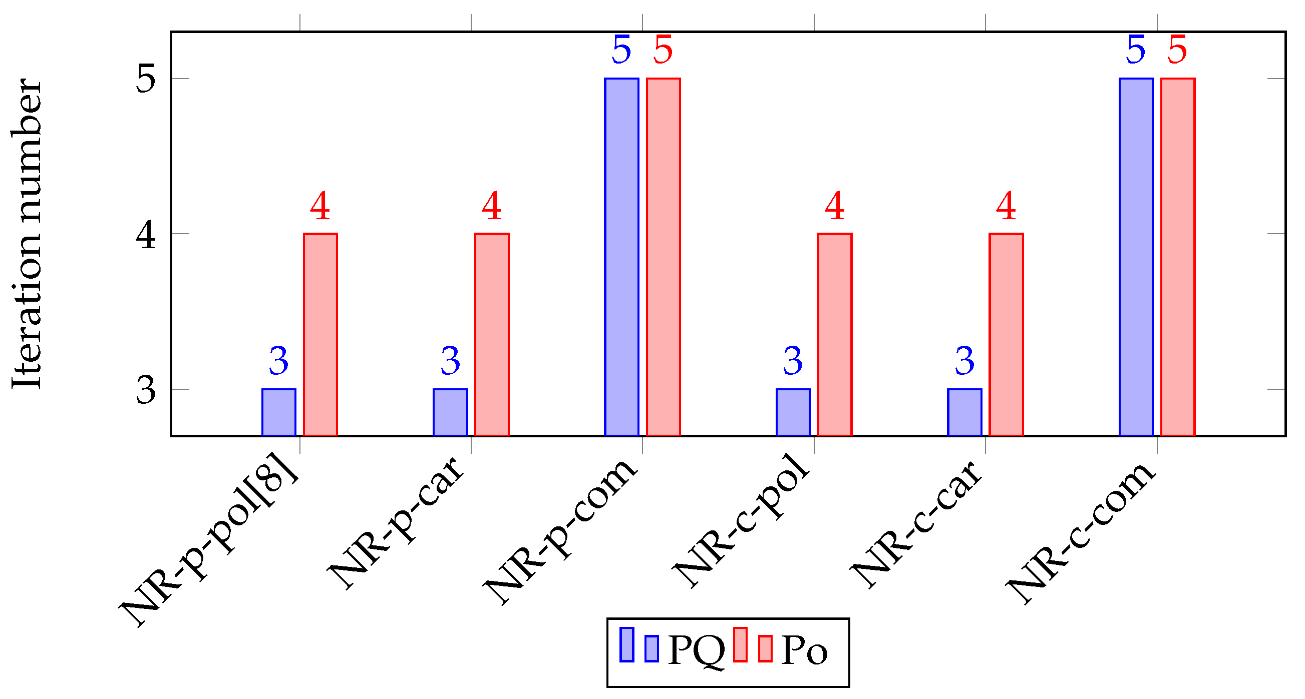
A convergence result of all solution methods for the unbalanced distribution network DCase13 with different loading conditions and different $R/X$ ratios is shown in Figure 8 and Figure 9, respectively. As in single-phase cases, NR-p-com and NR-c-com versions are more sensitive to the change of loads and $R/X$ ratios compared to other versions. Moreover, NR-c-pol and NR-c-car versions were more stable for the changes and therefore they can be applied to any unbalanced distribution networks with high $R/X$ ratios and loading conditions. All methods performed better when a constant power (PQ) model was applied to three-phase problems as shown in Figure 10. We can conclude that versions using the current mismatch functions (NR-c-pol and NR-c-car) are more suitable than versions using the power-mismatch functions (NR-p-pol [8] and NR-p-car) for unbalanced distribution networks.

6. Conclusions

In this paper, the Newton power flow methods developed for single-phase problems in [65] are extended to three-phase power flow problems. Mathematical models of the load, three-phase load connection, and three-phase transformer connection are studied and applied in the numerical experiments. The power flow problem is mathematically described for the three-phase problem. The Newton power flow method and its six possible versions are introduced for three-phase power flow problems. As one of the newly developed versions of the Newton power flow method, the polar current mismatch version (NR-c-pol) is explained in detail for a three-phase power flow problem. The existing version (NR-p-pol [8]) and the backward–forward sweep-based algorithm (BFS [43]) are applied for comparison purposes. As a result of the numerical experiment, the polar current mismatch (NR-c-pol) and the Cartesian current mismatch (NR-c-car) versions developed in [65] and extended in this paper perform the best for both balanced and unbalanced distribution networks. We also investigate which version can be applied to what kind of a power network by comparing all versions for distribution networks with different loading conditions, $R/X$ ratios, and load models. We observe that NR-c-pol and NR-c-car versions are more stable to the change of loading conditions and $R/X$ ratios for both balanced and unbalanced networks, whereas the performance of other methods is highly sensitive to them. Therefore, these two versions are the fastest and the most robust methods of other versions that can be applied to single or three-phase power flow problems in any balanced or unbalanced networks. For the subsequent research, these newly developed versions (NR-c-pol and NR-c-car) will be applied to the optimal power flow problem in hybrid networks including DGs as they result in new formulations for equality constraints.

References

- Schavemaker, P.; van der Sluis, L. Electrical Power System Essentials; Wiley: Hoboken, NJ, USA, 2008. [Google Scholar]
- Keyhani, A.; Marwali, M. Smart Power Grids 2011; Power Systems; Springer: Berlin, Germany, 2012. [Google Scholar]
- Budka, K.; Deshpande, J.; Thottan, M. Communication Networks for Smart Grids: Making Smart Grid Real; Computer Communications and Networks; Springer: Berlin, Germany, 2014. [Google Scholar]
- Thomas, M.; McDonald, J. Power System SCADA and Smart Grids; Taylor & Francis: Abingdon, UK, 2015. [Google Scholar]
- Balamurugan, K.; Srinivasan, D. Review of power flow studies on distribution network with distributed generation. In Proceedings of the 2011 IEEE Ninth International Conference on Power Electronics and Drive Systems, Singapore, 5–8 December 2011; pp. 411–417. [Google Scholar]
- Martinez, J.A.; Mahseredjian, J. Load flow calculations in distribution systems with distributed resources. A review. In Proceedings of the 2011 IEEE Power and Energy Society General Meeting, Detroit, MI, USA, 24–29 July 2011; pp. 1–8. [Google Scholar]
- Stevenson, W.D. Elements of Power System Analysis; McGraw-Hill: New York, NY, USA, 1975. [Google Scholar]
- Tinney, W.F.; Hart, C.E. Power flow solution by Newton’s method. IEEE Trans. Power Appar. Syst. 1967, PAS-86, 1449–1460. [Google Scholar] [CrossRef]
- Stott, B.; Alsaç, O. Fast decoupled load flow. IEEE Trans. Power Appar. Syst. 1974, PAS-93, 859–869. [Google Scholar] [CrossRef]
- Iwamoto, S.; Tamura, Y. A load flow calculation method for Ill-conditioned power systems. IEEE Trans. Power Appar. Syst. 1981, PAS-100, 1736–1743. [Google Scholar] [CrossRef]
- Tripathy, S.C.; Prasad, G.D.; Malik, O.P.; Hope, G.S. Load-flow solutions for ill-conditioned power systems by a newton-like method. IEEE Trans. Power Appar. Syst. 1982, PAS-101, 3648–3657. [Google Scholar] [CrossRef]
- Reddy, S.; Suresh, S.S.K.; Kumar, S.V.J. Load flow solution for ill-conditioned power systems using runge-kutta and Iwamoto methods with facts devices. J. Theor. Appl. Inf. Technol. 2009, 5, 693–703. [Google Scholar]
- Chiang, H.D. A decoupled load flow method for distribution power networks: Algorithms, analysis and convergence study. Int. J. Electr. Power Energy Syst. 1991, 13, 130–138. [Google Scholar] [CrossRef]
- Chen, T.H.; Chen, M.S.; Hwang, K.J.; Kotas, P.; Chebli, E.A. Distribution system power flow analysis—A rigid approach. IEEE Trans. Power Deliv. 1991, 6, 1146–1152. [Google Scholar] [CrossRef]
- Chen, T.H.; Chen, M.S.; Inoue, T.; Kotas, P.; Chebli, E.A. Three-phase cogenerator and transformer models for distribution system analysis. IEEE Trans. Power Deliv. 1991, 6, 1671–1681. [Google Scholar] [CrossRef]
- Zhang, F.; Cheng, C.S. A modified Newton method for radial distribution system power flow analysis. IEEE Trans. Power Syst. 1997, 12, 389–397. [Google Scholar] [CrossRef]
- Nguyen, H.L. Newton-Raphson method in complex form. IEEE Trans. Power Deliv. 1997, 12, 1355–1359. [Google Scholar] [CrossRef]
- Da Costa, V.M.; Martins, N.; Pereira, J.L.R. Developments in the Newton Raphson power flow formulation based on current injections. IEEE Trans. Power Syst. 1999, 14, 1320–1326. [Google Scholar] [CrossRef]
- Garcia, P.A.N.; Pereira, J.L.R.; Carneiro, S.; da Costa, V.M.; Martins, N. Three-phase power flow calculations using the current injection method. IEEE Trans. Power Syst. 2000, 15, 508–514. [Google Scholar] [CrossRef]
- Lin, W.M.; Teng, J.H. Three-phase distribution network fast-decoupled power flow solutions. Int. J. Electr. Power Energy Syst. 2000, 22, 375–380. [Google Scholar] [CrossRef]
- Teng, J.H.; Chang, C.Y. A novel and fast three-phase load flow for unbalanced radial distribution systems. IEEE Trans. Power Deliv. 2002, 17, 1238–1244. [Google Scholar] [CrossRef]
- Teng, J.H. A modified Gauss-Seidel algorithm of three-phase power flow analysis in distribution networks. Int. J. Electr. Power Energy Syst. 2002, 24, 97–102. [Google Scholar] [CrossRef]
- Vieira, J.; Freitas, W.; Morelato, A. Phase-decoupled method for three-phase power-flow analysis of unbalanced distribution systems. IEE Proc. Gener. Transm. Distrib. 2004, 151, 568–574. [Google Scholar] [CrossRef]
- Chen, T.H.; Yang, N.C. Loop frame of reference based three-phase power flow for unbalanced radial distribution systems. Electr. Power Syst. Res. 2010, 80, 799–806. [Google Scholar] [CrossRef]
- Sun, H.; Nikovski, D.; Ohno, T.; Takano, T.; Kojima, Y. A fast and robust load flow method for distribution systems with distributed generations. Energy Procedia 2011, 12, 236–244. [Google Scholar] [CrossRef]
- Lagace, P.J. Power flow methods for improving convergence. In Proceedings of the IECON 2012—38th Annual Conference on IEEE Industrial Electronics Society, Montreal, QC, Canada, 25–28 October 2012; pp. 1387–1392. [Google Scholar]
- Abdelaziz, M.M.A.; Farag, H.E.; El-Saadany, E.F.; Mohamed, Y.A.R.I. A novel and generalized three-phase power flow algorithm for islanded microgrids using a Newton trust region method. IEEE Trans. Power Syst. 2013, 28, 190–201. [Google Scholar] [CrossRef]
- Idema, R.; Lahaye, D. Computational Methods in Power System Analysis; Atlantis Studies in Scientific Computing in Electromagnetics; Atlantis Press: Amsterdam, The Netherlands, 2014. [Google Scholar]
- Li, C.; Chaudhary, S.K.; Vasquez, J.C.; Guerrero, J.M. Power flow analysis algorithm for islanded LV microgrids including distributed generator units with droop control and virtual impedance loop. In Proceedings of the 2014 IEEE Applied Power Electronics Conference and Exposition, Fort Worth, TX, USA, 16–20 March 2014; pp. 3181–3185. [Google Scholar]
- Wang, L.; Chen, C.; Shen, T. Improvement of power flow calculation with optimization factor based on current injection method. Discrete Dyn. Nat. Soc. 2014, 2014, 437567. [Google Scholar] [CrossRef]
- Milano, F. Analogy and convergence of Levenberg’s and Lyapunov-based methods for power flow analysis. IEEE Trans. Power Syst. 2016, 31, 1663–1664. [Google Scholar] [CrossRef]
- Mumtaz, F.; Syed, M.; Al Hosani, M.; Zeineldin, H. A novel approach to solve power flow for islanded microgrids using modified Newton-Raphson with droop control of DG. IEEE Trans. Sustain. Energy 2016, 7, 493–503. [Google Scholar] [CrossRef]
- Pourbagher, R.; Derakhshandeh, S.Y. A powerful method for solving the power flow problem in the ill-conditioned systems. Int. J. Electr. Power Energy Syst. 2018, 94, 88–96. [Google Scholar] [CrossRef]
- Cheng, C.S.; Shirmohammadi, D. A three-phase power flow method for real-time distribution system analysis. IEEE Trans. Power Deliv. 1995, 10, 671–679. [Google Scholar] [CrossRef]
- Thukaram, D.; Banda, H.W.; Jerome, J. A robust three phase power flow algorithm for radial distribution systems. Electr. Power Syst. Res. 1999, 50, 227–236. [Google Scholar] [CrossRef]
- Ranjan, R.; Venkatesh, B.; Chaturvedi, A.; Das, D. Power flow solution of three-phase unbalanced radial distribution network. Electr. Power Compon. Syst. 2004, 32, 421–433. [Google Scholar] [CrossRef]
- Khushalani, S.; Solanki, J.M.; Schulz, N.N. Development of three-phase unbalanced power flow using PV and PQ models for distributed generation and study of the impact of DG models. IEEE Trans. Power Deliv. 2007, 22, 1019–1025. [Google Scholar] [CrossRef]
- Moghaddas-Tafreshi, S.; Mashhour, E. Distributed generation modeling for power flow studies and a three-phase unbalanced power flow solution for radial distribution systems considering distributed generation. Electr. Power Syst. Res. 2009, 79, 680–686. [Google Scholar] [CrossRef]
- Shirmohammadi, D.; Hong, H.; Semlyen, A.; Luo, G. A compensation-based power flow method for weakly meshed distribution and transmission networks. IEEE Trans. Power Deliv. 1988, 3, 753–762. [Google Scholar] [CrossRef]
- Luo, G.X.; Semlyen, A. Efficient load flow for large weakly meshed networks. IEEE Trans. Power Syst. 1990, 5, 1309–1316. [Google Scholar] [CrossRef]
- Haque, M.H. Efficient load flow method for distribution systems with radial or mesh configuration. IEE Proc. Gener. Transm. Distrib. 1996, 143, 33–38. [Google Scholar] [CrossRef]
- Haque, M. A general load flow method for distribution systems. Electr. Power Syst. Res. 2000, 54, 47–54. [Google Scholar] [CrossRef]
- Teng, J.H. A direct approach for distribution system load flow solutions. IEEE Trans. Power Deliv. 2003, 18, 882–887. [Google Scholar] [CrossRef]
- Rajicic, D.; Ackovski, R.; Taleski, R. Voltage correction power flow. IEEE Trans. Power Deliv. 1994, 9, 1056–1062. [Google Scholar] [CrossRef]
- Zhu, Y.; Tomsovic, K. Adaptive power flow method for distribution systems with dispersed generation. IEEE Trans. Power Deliv. 2002, 17, 822–827. [Google Scholar] [CrossRef]
- Teng, J.H. Modelling distributed generations in three-phase distribution load flow. IET Proc. Gener. Transm. Distrib. 2008, 2, 330–340. [Google Scholar] [CrossRef]
- Augugliaro, A.; Dusonchet, L.; Favuzza, S.; Ippolito, M.; Sanseverino, E.R. A new backward/forward method for solving radial distribution networks with PV nodes. Electr. Power Syst. Res. 2008, 78, 330–336. [Google Scholar] [CrossRef]
- Ghosh, S.; Das, D. Method for load-flow solution of radial distribution networks. IEE Proc. Gener. Transm. Distrib. 1999, 146, 641–648. [Google Scholar] [CrossRef]
- Samuel Mok, S.; Elangovan, C.L.; Salama, M. A new approach for power flow analysis of balanced radial distribution systems. Electr. Mach. Power Syst. 2000, 28, 325–340. [Google Scholar]
- Aravindhababu, P.; Ganapathy, S.; Nayar, K. A novel technique for the analysis of radial distribution systems. Int. J. Electr. Power Energy Syst. 2001, 23, 167–171. [Google Scholar] [CrossRef]
- Liu, J.; Salama, M.; Mansour, R. An efficient power flow algorithm for distribution systems with polynomial load. Int. J. Electr. Eng. Educ. 2002, 39, 371–386. [Google Scholar] [CrossRef]
- Cespedes, R. New method for the analysis of distribution networks. IEEE Trans. Power Deliv. 1990, 5, 391–396. [Google Scholar] [CrossRef]
- Jasmon, G.; Lee, L. Distribution network reduction for voltage stability analysis and loadflow calculations. Int. J. Electr. Power Energy Syst. 1991, 13, 9–13. [Google Scholar] [CrossRef]
- Das, D.; Nagi, H.; Kothari, D. Novel method for solving radial distribution networks. IEE Proc. Gener. Transm. Distrib. 1994, 141, 291–298. [Google Scholar] [CrossRef]
- Das, D.; Kothari, D.; Kalam, A. Simple and efficient method for load flow solution of radial distribution networks. Int. J. Electr. Power Energy Syst. 1995, 17, 335–346. [Google Scholar] [CrossRef]
- Haque, M. Load flow solution of distribution systems with voltage dependent load models. Electr. Power Syst. Res. 1996, 36, 151–156. [Google Scholar] [CrossRef]
- Afsari, M.; Singh, S.; Raju, G.; Rao, G. A fast power flow solution of radial distribution networks. Electr. Power Compon. Syst. 2002, 30, 1065–1074. [Google Scholar] [CrossRef]
- Mekhamer, S.; Soliman, S.; Moustafa, M.; El-Hawary, M. Load flow solution of radial distribution feeders: A new contribution. Int. J. Electr. Power Energy Syst. 2002, 24, 701–707. [Google Scholar] [CrossRef]
- Ranjan, R.; DAS. Simple and efficient computer algorithm to solve radial distribution networks. Electr. Power Compon. Syst. 2003, 31, 95–107. [Google Scholar] [CrossRef]
- Eminoglu, U.; Hocaoglu, M.H. A new power flow method for radial distribution systems including voltage dependent load models. Electr. Power Syst. Res. 2005, 76, 106–114. [Google Scholar] [CrossRef]
- Satyanarayana, S.; Ramana, T.; Sivanagaraju, S.; Rao, G. An efficient load flow solution for radial distribution network including voltage dependent load models. Electr. Power Compon. Syst. 2007, 35, 539–551. [Google Scholar] [CrossRef]
- Stott, B. Review of load-flow calculation methods. Proc. IEEE 1974, 62, 916–929. [Google Scholar] [CrossRef]
- Srinivas, M.S. Distribution load flows: A brief review. In Proceedings of the 2000 IEEE Power Engineering Society Winter Meeting, Singapore, 23–27 January 2000; Volume 2, pp. 942–945. [Google Scholar]
- Eminoglu, U.; Hocaoglu, M.H. Distribution systems forward/backward sweep-based power flow algorithms: A review and comparison study. Electr. Power Compon. Syst. 2008, 37, 91–110. [Google Scholar] [CrossRef]
- Sereeter, B.; Vuik, C.; Witteveen, C. On a Comparison of Newton-Raphson Solvers for Power Flow Problems; Report 17-7; Delft Institute of Applied Mathematics, Delft University of Technology: Delft, The Netherlands, 2017. [Google Scholar]
- Van Ness, J.E.; Griffin, J.H. Elimination methods for load-flow studies. Trans. Am. Inst. Electr. Eng. Part III 1961, 80, 299–302. [Google Scholar] [CrossRef]
- Lindén, K.; Segerqvist, I. Modelling of Load Devices and Studying Load/System Characteristics; Technical Report; Chalmers University of Technology: Gothenburg, Sweden, 1992. [Google Scholar]
- Subrahmanyam, J.; Radhakrishna, C. A simple approach of three phase distribution system modeling for power flow calculations. Int. J. Energy Power Eng. 2010, 3, 3. [Google Scholar]
- Electric Power Research Institute (EPRI). Engineering Guide for Integration of Distributed Generation and Storage into Power Distribution Systems; Technical Report; EPRI: Palo Alto, CA, USA, 2000. [Google Scholar]
- Baran, M.E.; Wu, F.F. Network reconfiguration in distribution systems for loss reduction and load balancing. IEEE Trans. Power Deliv. 1989, 4, 1401–1407. [Google Scholar] [CrossRef]
- Baran, M.E.; Wu, F.F. Optimal capacitor placement on radial distribution systems. IEEE Trans. Power Deliv. 1989, 4, 725–734. [Google Scholar] [CrossRef]
- Kersting, W.H. Radial distribution test feeders. In Proceedings of the 2001 IEEE Power Engineering Society Winter Meeting, Columbus, OH, USA, 28 January–1 February 2001; Volume 2, pp. 908–912. [Google Scholar]
Figure 1.
Wye and delta connections for three-phase loads [68].
Figure 2.
Combination of power converters and energy sources [69].
Figure 3.
Flow chart of the polar current mismatch version.
Figure 4.
Computed voltage magnitude of DCase69. (a) Computed voltage magnitude ; (b) Difference between proposed methods and existing method [48] for the computed voltage magnitude.
Figure 5.
Convergence results for different loading conditions () in DCase69.
Figure 6.
Convergence results for different ratios () in DCase69.
Figure 7.
Convergence result for different load models (constant power (PQ) and polynomial (Po)) in DCase69.
Figure 8.
Convergence results for different loading conditions () in DCase13.
Figure 9.
Convergence results for different ratios () in DCase13.
Figure 10.
Convergence result for different load models (constant power (PQ) and polynomial (Po)) in DCase13.