A Multi-Energy System Expansion Planning Method Using a Linearized Load-Energy Curve: A Case Study in South Korea

Abstract

Multi-energy systems can integrate heat and electrical energy efficiently, using resources such as cogeneration. In order to meet energy demand cost-effectively in a multi-energy system, adopting appropriate energy resources at the right time is of great importance. In this paper, we propose an expansion planning method for a multi-energy system that supplies heat and electrical energy. The proposed approach formulates expansion planning as a mixed integer linear programming (MILP) problem. The objective is to minimize the sum of the annualized cost of the multi-energy system. The candidate resources that constitute the cost of the multi-energy system are fuel-based power generators, heat-only boilers, a combined heat and power (CHP) unit, energy storage resources, and a renewable electrical power source. We use a load-energy curve, instead of a load-duration curve, for constructing the optimization model, which is subsequently linearized using a Douglas-Peucker algorithm. The residual load-energy curve, for utilizing the renewable electrical power source, is also linearized. This study demonstrates the effectiveness of the proposed method through a comparison with a conventional linearization method. In addition, we evaluate the cost and planning schedules of different case studies, according to the configuration of resources in the multi-energy system.

1. Introduction

With the increased emphasis on energy efficiency under current environmental policy, there has been growing interest in systems that can efficiently supply and consume energy. In the operation and planning of conventional energy systems, single energy sources are typically considered individually, though these sources have interdependencies [1]. In addition, as a result of economic and environmental concerns, energy systems tend to operate in a decentralized manner. Recently, the multi-energy system concept has been introduced [2]. In a multi-energy system, electricity, heat, and gas sources are treated interdependently. The cost of fuel and the availability of power from a gas turbine power plant depend on the price of gas and the status of the gas supply facility, respectively [3]. It has been noted that combined heat and power (CHP) systems could afford significant energy efficiency by producing heat and electricity from a single fuel, including natural gas [4]. In urban regions where various energy sources, including district heat, electricity, and natural gas, are consumed, CHP systems can improve the environmental performances. For example, these systems can avoid the use of methane hydrate by providing other resources with heat for preheating of natural gas [5,6]. In addition, thermal energy storage decouples the supply of electrical energy from that of heat energy when a cogeneration unit is used, thereby improving the efficiency of energy supply [7]. To efficiently use these facilities in multi-energy systems, it is necessary to make a plan for each energy sector.

Many studies have investigated the integrated operation and planning of gas and electricity supplies. From the perspective of system operation, generator commitment was determined on the basis of the status of gas pipes [3]. In contrast, in the integrated energy expansion planning process detailed in [8,9], the construction of generators, gas wells, gas pipes, and gas tanks was also considered to meet the gas demand, including the demand for gas as a fuel for generators. Integrated operation and planning of heat and electricity have also been studied. The optimal operating conditions required for heat-only boilers, fuel-based generators, and CHP units to meet heat and electricity demand, were determined [10]. Expansion planning of CHP units was also considered in terms of the amount of heat and electricity consumed [11]. The model in [12] was proposed to design an energy integrated multi-microgrid system that could provide microgrid operation and heating pipelines to meet heat and electricity demand. There have also been studies on energy hubs that can integrate multiple forms of energy such as, gas, heat, and electricity [13]. The method discussed in [14] was used to design an energy hub comprising CHP units and other thermal and electrical resources considering reliability constraints. In contrast, an optimal operation strategy in multiple energy hub systems considered the efficiency of energy conversion and the price of electricity [15]. Furthermore, a model called an energy internet in [16] was based on the energy hub and was proposed to consider dynamic operation of multiple energy flows. Although it is desirable to consider all forms of energy in the operation and planning of an energy system, the focus is predominantly on heat and electrical energy, as gas is converted into these forms of energy.

Expansion planning models for heat and electrical systems have been designed to minimize the investment and operation cost of energy resources. In [17], the integrated expansion planning method was applied in a case study on the Alberta region (Canada), where many CHP units might be used. Furthermore, other models detailed in [18,19] were designed to minimize energy loss and voltage fluctuation, as well as cost. The study in [20] proposed an expansion planning model for distributed multi-energy generation to cope with long-term uncertainty, including operation and investment flexibility. A notable feature of the expansion planning method proposed in [21] was the consideration of CHP units and boilers in a district energy system to provide heat and electricity. Expansion planning methods were also proposed in [14,22] to determine the requisite size of energy hub facilities, including CHP units, boilers, and energy storage resources. However, these methods rarely consider resources other than those detailed above. It is necessary to consider a variety of energy resources in expansion planning, as energy systems can potentially adopt a wider range of resources than those listed.

The expansion planning problem can be modeled as a mixed integer linear programming (MILP) problem, which can be formulated by linearizing the constraints. Linearization is realized by selecting typical days in project years instead of using an entire year of demand data [14,20,22], or by using a stepwise representation of a load duration curve (LDC) [23]. Although it is better to linearize the curve as closely as possible to the original data, the computational burden increases with the number of linearization segments [24]. Linearization is important in the MILP problem; however, there is no consistent standard for how to select typical days or how to construct a stepwise function.

This paper proposes a method to model an expansion planning problem for a multi-energy system where energy resources supply the heat and electricity demand. Furthermore, in this model, we focus on the method of planning energy resources on an annual basis rather than an hourly basis, because we suggest a method of designing rather than operating a multi-energy system. Therefore, this paper will cover the following:

• The expansion planning problem for a multi-energy system, where considering various energy resources, including fuel-based generators and a renewable electrical power source, as well as a CHP unit and energy storage resources, is modeled as an MILP problem with linearized constraints.
• To model linearized constraints including a linearized load curve, we use a load-energy curve instead of the LDC, and apply a Douglas-Peucker algorithm that can approximate linear functions and minimize the distortion of the original demand function.
• To validate the use of a linearized load-energy curve, the results of optimization methods using the linearized load-energy curve and the stepwise representation of LDC are compared.
• A case study for a multi-energy system based on a benchmark case from Goyang city in South Korea is presented.

The rest of this paper is organized as follows: Section 2 presents the multi-energy system considered in this paper. An objective function and basic models of the resources are described in Section 3; In Section 4, we introduce the load-energy curve, which is used instead of a load-duration curve in the expansion planning problem, and linearization using the Douglas-Peucker algorithm; The optimization process and a comparison of the proposed optimization method with a conventional method are shown in Section 5; The proposed method is illustrated with several case studies, in Section 6; The conclusions of this paper are presented in Section 7.

2. Multi-Energy System Overview

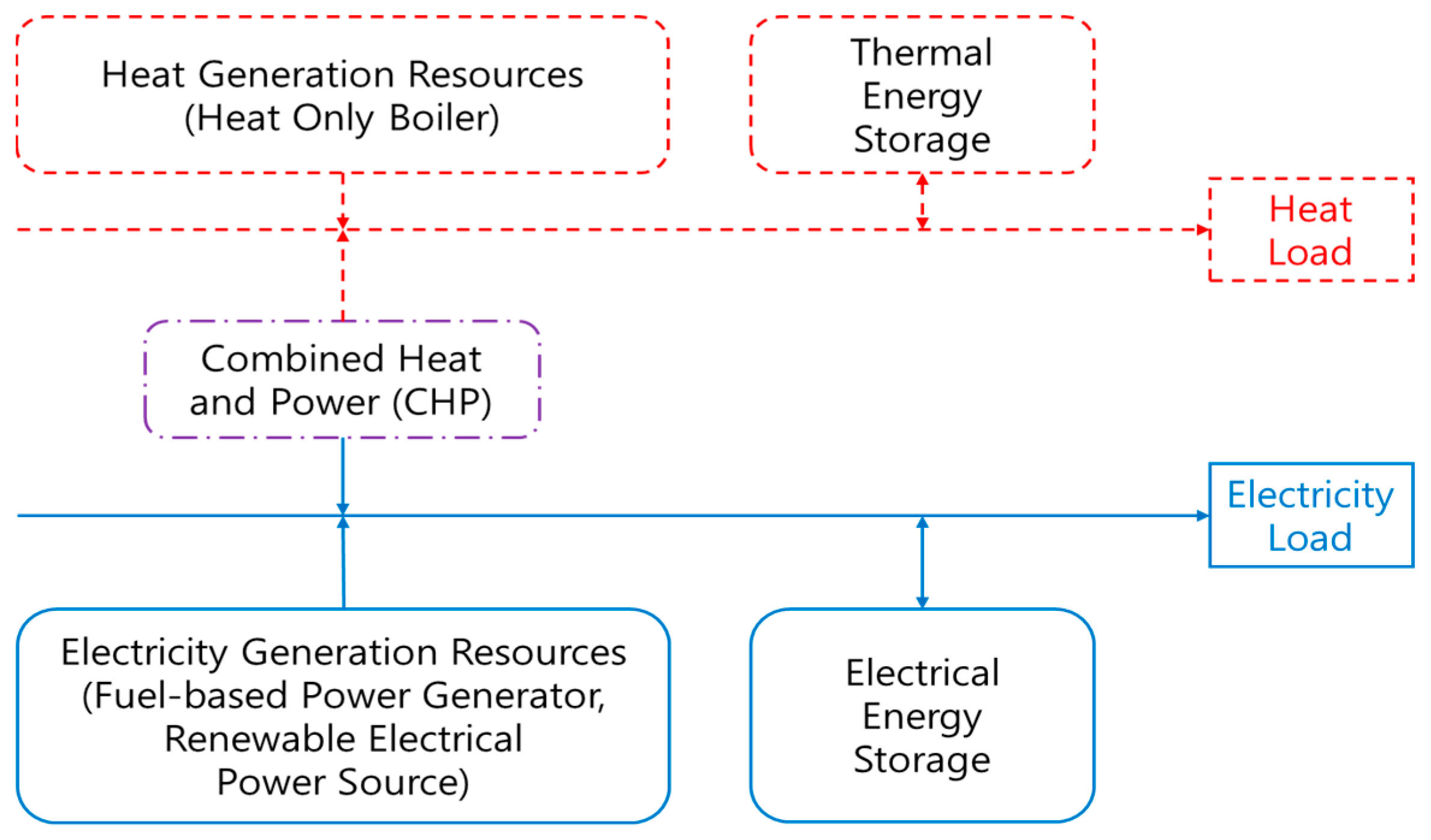
Multi-energy systems have been modeled in various forms. The distributed multi-energy generation system in [20] and the energy hub model in [25] were composed of heat and electricity networks, including CHP units, boilers, and storage resources. Based on the configuration of these models, the multi-energy system model in this work also consists of a heat and an electricity network. In addition, to utilize various energy resources except CHP units, boilers, and storage resources included in conventional models, this model is assumed to represent a self-sufficient system, and this system is then modeled as shown in Figure 1. This model is composed of the heat and electricity network, identified using dashed lines and solid lines, respectively. In this work, the energy generation resources for supplying heat or electricity are assumed to be unidirectional components. A renewable energy source is also considered, particularly with respect to electricity generation, because this resource is expected to be widely used to reduce the primary energy consumption, as shown in [26]. Furthermore, in [27], the excess electricity due to generation of this resource could be converted to heat. Although utilization of this resource can involve various energy transitions and conversions, this resource is assumed to produce only electricity, because our model cannot yet consider fuel usage or energy transitions caused by other resources except the CHP unit. We note that the CHP unit, identified using the dash-dotted line, can generate thermal and electrical energy simultaneously. In addition, because the energy storage resources can charge or discharge energy, they are configured as bidirectional components.

3. Basic Optimization Model

This section introduces the objective function and the basic resource model for a multi-energy system expansion planning problem modeled using MILP.

3.1. Objective Function

The objective of the multi-energy system expansion planning problem is to define the optimum energy generation mix, and to minimize the sum of the annualized costs, including the initial investment and operation costs of all energy resources, over the planning horizon, $N_Y$. The objective function is modelled as:

$$\mathrm{Minimize}{\displaystyle \sum _{y=1}^{N_Y}\left({\mathrm{COST}}_e^y+{\mathrm{COST}}_h^y+{\mathrm{COST}}_{\mathrm{CHP}}^y\right)}$$

(1)

where, ${\mathrm{COST}}_e^y$, ${\mathrm{COST}}_h^y$, and ${\mathrm{COST}}_{\mathrm{CHP}}^y$ are the respective sums of the annualized investment and the operational costs for electrical energy, heat energy, and the CHP unit for the planning year, $y$. Each cost consists of a fixed component, including capital and fixed operation and maintenance costs relating to the capacity of a resource, and a variable component, including fuel costs and variable operation and maintenance costs relating to the utilized energy of a resource, and is defined as below:

$$\begin{array}{c}{\mathrm{COST}}_e^y={\displaystyle \sum _{i=1}^{N_{ER}}\left(1-{\rho }_{\mathrm{CHP},e}^i\right)\cdot {\left(1+{\gamma }_d\right)}^{-y}\cdot \left(CR{F}^i\cdot C{C}_e^i+FOM{C}_e^i\right)\cdot \left[{\displaystyle \sum _{c=1}^{N_C}{C}_e^{i,c}\cdot {\nu }_e^{i,c,y}}\right]}\\ +{\displaystyle \sum _{i=1}^{N_{ER}}\left(1-{\rho }_{\mathrm{CHP},e}^i\right)\cdot {\left(1+{\gamma }_d\right)}^{-y}\cdot \left(F{C}_e^i+VOM{C}_e^i\right)\cdot \left[{\displaystyle \sum _{si=1}^{N_{EST}}{E}_e^{i,si,y}}\right]}\end{array}\hspace{1em}\forall y$$

(2)

$$\begin{array}{c}{\mathrm{COST}}_h^y={\displaystyle \sum _{j=1}^{N_{HR}}\left(1-{\rho }_{\mathrm{CHP},h}^j\right)\cdot {\left(1+{\gamma }_d\right)}^{-y}\cdot \left(CR{F}^j\cdot C{C}_h^j+FOM{C}_h^j\right)\cdot \left[{\displaystyle \sum _{c=1}^{N_C}{C}_h^{j,c}\cdot {\nu }_h^{j,c,y}}\right]}\\ +{\displaystyle \sum _{j=1}^{N_{HR}}\left(1-{\rho }_{\mathrm{CHP},h}^j\right)\cdot {\left(1+{\gamma }_d\right)}^{-y}\cdot \left(F{C}_h^j+VOM{C}_h^j\right)\cdot \left[{\displaystyle \sum _{sj=1}^{N_{HST}}{E}_h^{j,sj,y}}\right]}\end{array}\hspace{1em}\forall y$$

(3)

$$\begin{array}{c}{\mathrm{COST}}_{\mathrm{CHP}}^y={\displaystyle \sum _{i=1}^{N_{ER}}{\rho }_{\mathrm{CHP},e}^i\cdot {\left(1+{\gamma }_d\right)}^{-y}\cdot \left(CR{F}^i\cdot C{C}_e^i+FOM{C}_e^i\right)\cdot \left[{\displaystyle \sum _{c=1}^{N_C}{C}_e^{i,c}\cdot {\nu }_e^{i,c,y}}\right]}\\ +{\displaystyle \sum _{i=1}^{N_{ER}}{\rho }_{\mathrm{CHP},e}^i\cdot {\left(1+{\gamma }_d\right)}^{-y}\cdot \left(F{C}_e^i+VOM{C}_e^i\right)\cdot \left[{\displaystyle \sum _{si=1}^{N_{EST}}{E}_e^{i,si,y}}\right]}\end{array}\hspace{1em}\forall y$$

(4)

where:

$$CR{F}_e^i=\frac{{\gamma }_d{\left(1+{\gamma }_d\right)}^{L{T}_e^i}}{{\left(1+{\gamma }_d\right)}^{L{T}_e^i}-1}, CR{F}_h^j=\frac{{\gamma }_d{\left(1+{\gamma }_d\right)}^{L{T}_h^j}}{{\left(1+{\gamma }_d\right)}^{L{T}_h^j}-1}\hspace{1em}\forall i,\forall j.$$

(5)

Equations (2)–(4) show the total cost of resources, including fixed costs and variable costs. Fixed costs consist of the candidate capacity of the electrical and heat energy resources, $C_e^{i,c}$, $C_h^{j,c}$, the overnight capital costs, $C{C}_e^i$, $C{C}_h^j$, the capital recovery factor defined in Equation (5), $CR{F}_e^i$, $CR{F}_h^j$, and the fixed operation and maintenance costs, $FOM{C}_e^i$, $FOM{C}_h^j$. In the same way, the variable costs for the planning year consist of the utilized energy, $E_e^{i,si,y}$, $E_h^{j,sj,y}$, the cost of fuel, $F{C}_e^i$, $F{C}_h^j$, and the variable operation and maintenance cost, $VOM{C}_e^i$, $VOM{C}_h^j$. Besides, in modeling fixed costs and variable costs for the planning year, we apply the interest rate, ${\gamma }_d$.

As the CHP unit is capable of generating heat and electricity simultaneously, it can be classified either as a heat generation resource or an electricity generation. Hence, the cost of the CHP unit should be calculated separately, because the objective function contains the cost of the heat generation resources and the electricity generation resources. As shown in Equations (2) and (3), the contribution of the CHP unit to the total cost of the heat generation and electricity generation resources can be split, by introducing an index for the CHP unit, ${\rho }_{\mathrm{CHP},e}^i$, ${\rho }_{\mathrm{CHP},h}^j$. Therefore, the total cost of the CHP unit can be calculated using Equation (4).

3.2. CHP Constraints

The allocation of resources for heat and electricity is influenced by the CHP unit, as this resource can generate heat and electricity simultaneously. The heat-to-power ratio, ${\alpha }_{HPR}$, determines the proportion of the heat and electricity output supplied by the CHP unit. Although it would vary with the heat and electricity output in hourly operation, it is assumed to have a constant value when the expected heat and electricity output of the CHP unit during a project year is considered, because the expansion planning problem in this work is not designed to consider hourly operation of the multi-energy system. It governs the amount of heat and electrical energy contributed to the desired capacity and the utilized energy, as shown in Equations (6) and (7):

$${\displaystyle \sum _{i=1}^{N_{ER}}\left({\rho }_{\mathrm{CHP},e}^i\cdot {\alpha }_{HPR}\cdot \left[{\displaystyle \sum _{si=1}^{N_{EST}}{P}_e^{i,si,y}}\right]\right)}={\displaystyle \sum _{j=1}^{N_{HR}}\left({\rho }_{\mathrm{CHP},h}^j\cdot \left[{\displaystyle \sum _{sj=1}^{N_{HST}}{P}_h^{j,sj,y}}\right]\right)}\hspace{1em}\forall y$$

(6)

$${\displaystyle \sum _{i=1}^{N_{ER}}\left({\rho }_{\mathrm{CHP},e}^i\cdot {\alpha }_{HPR}\cdot \left[{\displaystyle \sum _{si=1}^{N_{EST}}{E}_e^{i,si,y}}\right]\right)}={\displaystyle \sum _{j=1}^{N_{HR}}\left({\rho }_{\mathrm{CHP},h}^j\cdot \left[{\displaystyle \sum _{sj=1}^{N_{HST}}{E}_h^{j,sj,y}}\right]\right)}\hspace{1em}\forall y.$$

(7)

3.3. Energy Storage Constraints

Although energy storage resources in this system are similar to other resources from the perspective of estimating the utilized energy, they are charged from other resources, to discharge energy. Because the stored energy is designed to be completely discharged during the project year, the charging energy must be equal to the discharging energy, as in the definition below:

$${\displaystyle \sum _{i=1}^{N_{ER}}\left({\rho }_{EES}^i\cdot \left[{\displaystyle \sum _{si=1}^{N_{EST}}{E}_e^{i,si,y}}\right]\right)}={\displaystyle \sum _{i=1}^{N_{EST}}{e}_{EES}^{si,y}}, {\displaystyle \sum _{j=1}^{N_{HR}}\left({\rho }_{TES}^j\cdot \left[{\displaystyle \sum _{sj=1}^{N_{HST}}{E}_h^{j,sj,y}}\right]\right)}={\displaystyle \sum _{j=1}^{N_{HST}}{e}_{TES}^{sj,y}}\hspace{1em}\forall y.$$

(8)

In addition, since unlike other resources, the energy storage resources do not generate the energy required for charging, the range of charging energy can be defined as:

$$0\le e_{EES}^{si,y}\le {\displaystyle \sum _{i=1}^{N_{ER}}\left(\left(1-{\rho }_{EES}^i\right)\cdot E_e^{i,si,y}\right)}, 0\le e_{TES}^{sj,y}\le {\displaystyle \sum _{j=1}^{N_{HR}}\left(\left(1-{\rho }_{TES}^j\right)\cdot E_h^{j,sj,y}\right)}\hspace{1em}\forall si,\forall sj,\forall y.$$

(9)

3.4. Lifespan Constraints

The resource scheduled to be installed is designed to run continuously during its life span, and retired if it reaches the end of its life. In mathematical expression, the allocated candidate unit should operate for at least its lifetime, as follows:

$$\begin{gathered} {\displaystyle \sum _{t=y}^{Min(N_Y,y+L{T}_e^i-1)}{\nu }_e^{i,c,t}}\ge L{T}_e^i\cdot \left({\nu }_e^{i,c,y}-{\nu }_e^{i,c,y-1}\right)\hspace{1em}\forall i,\forall c,\forall y, (v_e^{i,c,0}=0), \\ {\displaystyle \sum _{t=y}^{Min(N_Y,y+L{T}_h^j-1)}{\nu }_h^{j,c,t}}\ge L{T}_h^j\cdot \left({\nu }_h^{j,c,y}-{\nu }_h^{j,c,y-1}\right)\hspace{1em}\forall j,\forall c,\forall y, (v_h^{j,c,0}=0). \end{gathered}$$

(10)

In contrast with deciding the operating period of an allocated candidate unit individually, the year of retirement for the allocated candidate unit is determined by comparing its life span with the cumulative operating year, as below:

$${\displaystyle \sum _{t=Max\left(1,y-L{T}_e^i\right)}^{Max\left(1,y\right)}{\nu }_e^{i,c,t}}\le L{T}_e^i,{\displaystyle \sum _{t=Max\left(1,y-L{T}_h^j\right)}^{Max\left(1,y\right)}{\nu }_h^{j,c,t}}\le L{T}_h^j\hspace{1em}\forall i,\forall c,\forall y.$$

(11)

4. Linearized Load-Energy Curve

In this work, expansion planning is formulated as an MILP problem. For accurate modeling, because the amount of load demand and that of energy demand are used to determine the installed capacity and the utilized energy of candidate resources, respectively, it is important that these values can be extracted precisely from a load curve. The load curve must also be modeled considering the renewable electrical power source, which is treated as a negative load.

4.1. Load-Energy Curve and Linearization

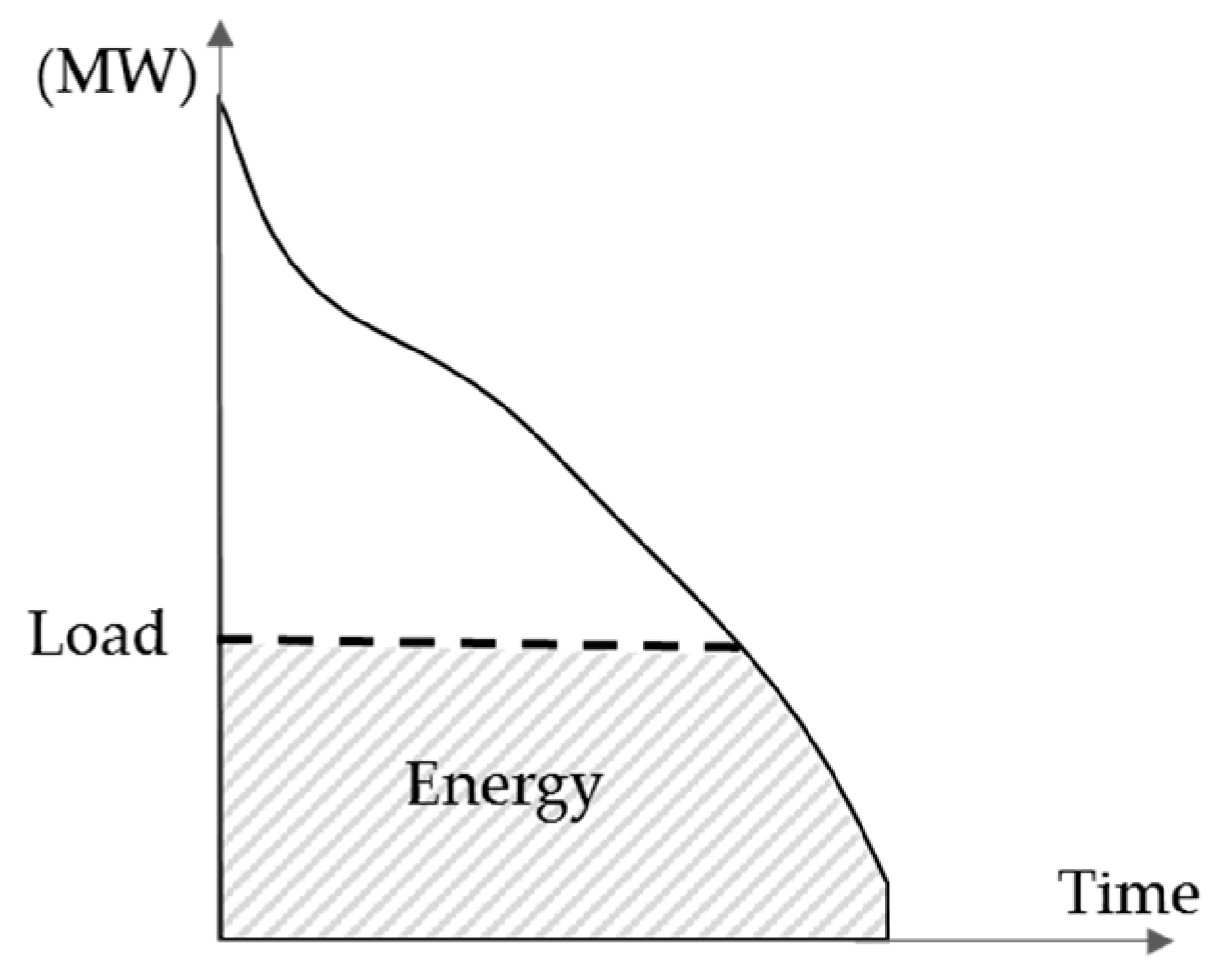
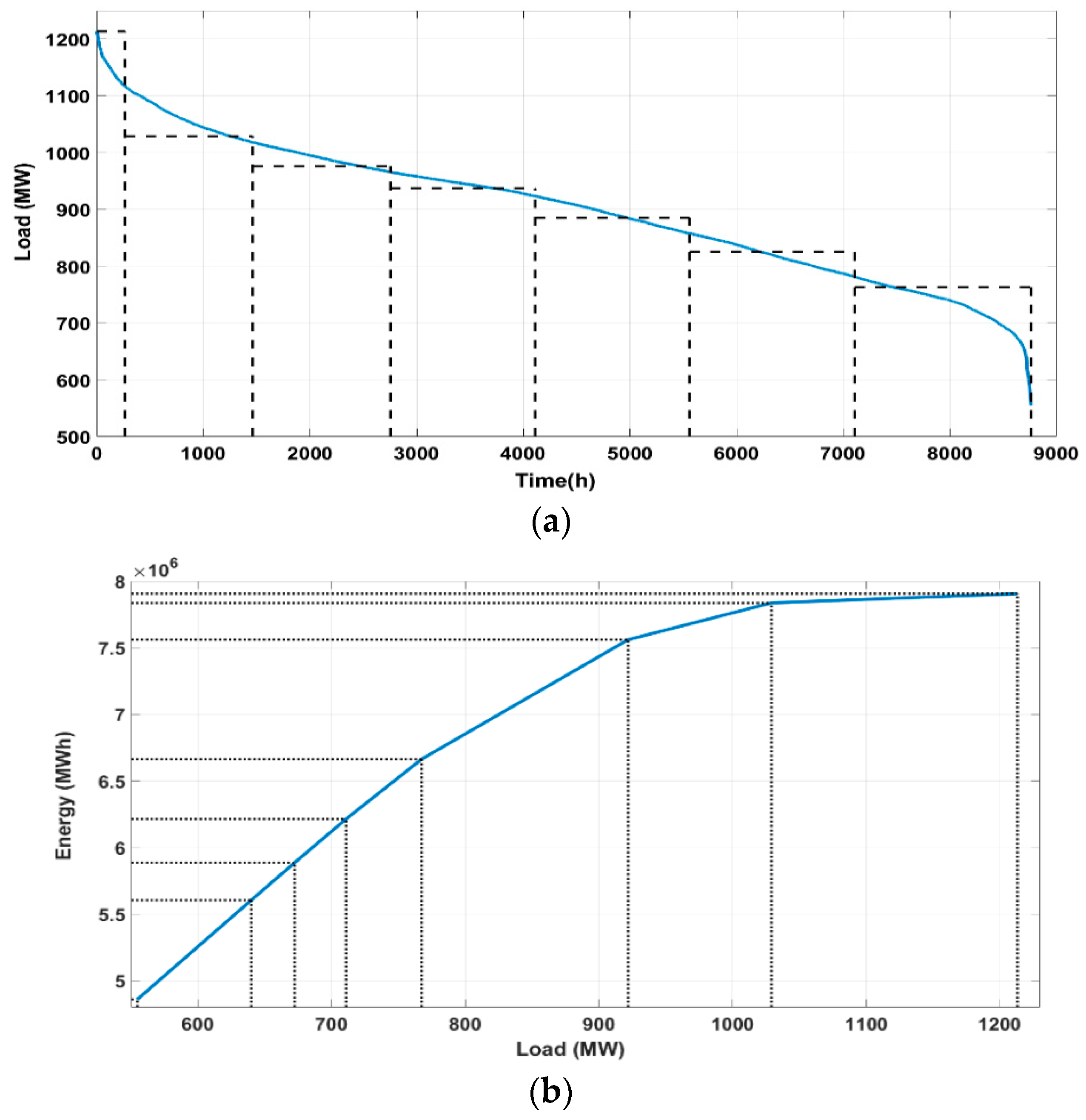
Figure 2 shows the LDC known to be useful to formulate the expansion planning problem. This curve represents the amount of time that the available capacity of the energy resources exceeds a given load demand. The load values are arranged in descending order, and energy is obtained by integrating the load with respect to time, as shown in Figure 2. This method of calculating the energy makes expansion planning a non-linear programming problem. For this reason, a step-wise representation of the LDC was used to formulate the MILP problem in [28,29]. Although these stepwise curves might appear to be similar, the approximation methods for modeling them were not consistent; in these methods, the number of steps and the step size for minimizing the approximation error were estimated randomly.

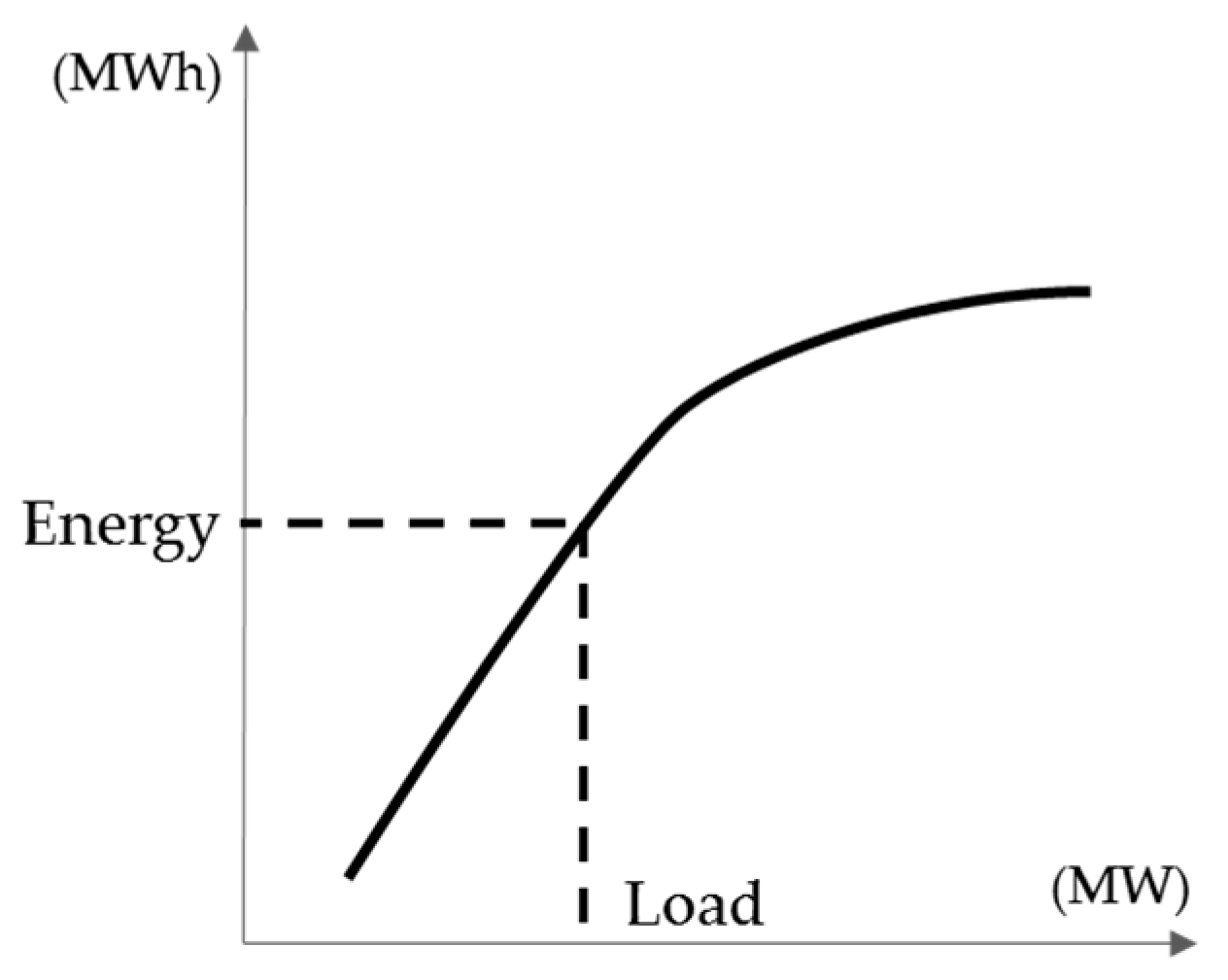
In order to avoid the problem mentioned above, we use a load-energy curve, which illustrates the relationship between load and energy, instead of the LDC. An illustrative load-energy curve is depicted in Figure 3. The load of this curve is equal to that of the LDC, while the energy is calculated by the integral of the load with respect to the corresponding utilization time in the LDC. Contrary to determining the energy in the LDC, it can be seen from Figure 3 that the energy can be determined according to the load, without an integration process. This feature can be used for direct assignment of the utilized energy in the optimization problem.

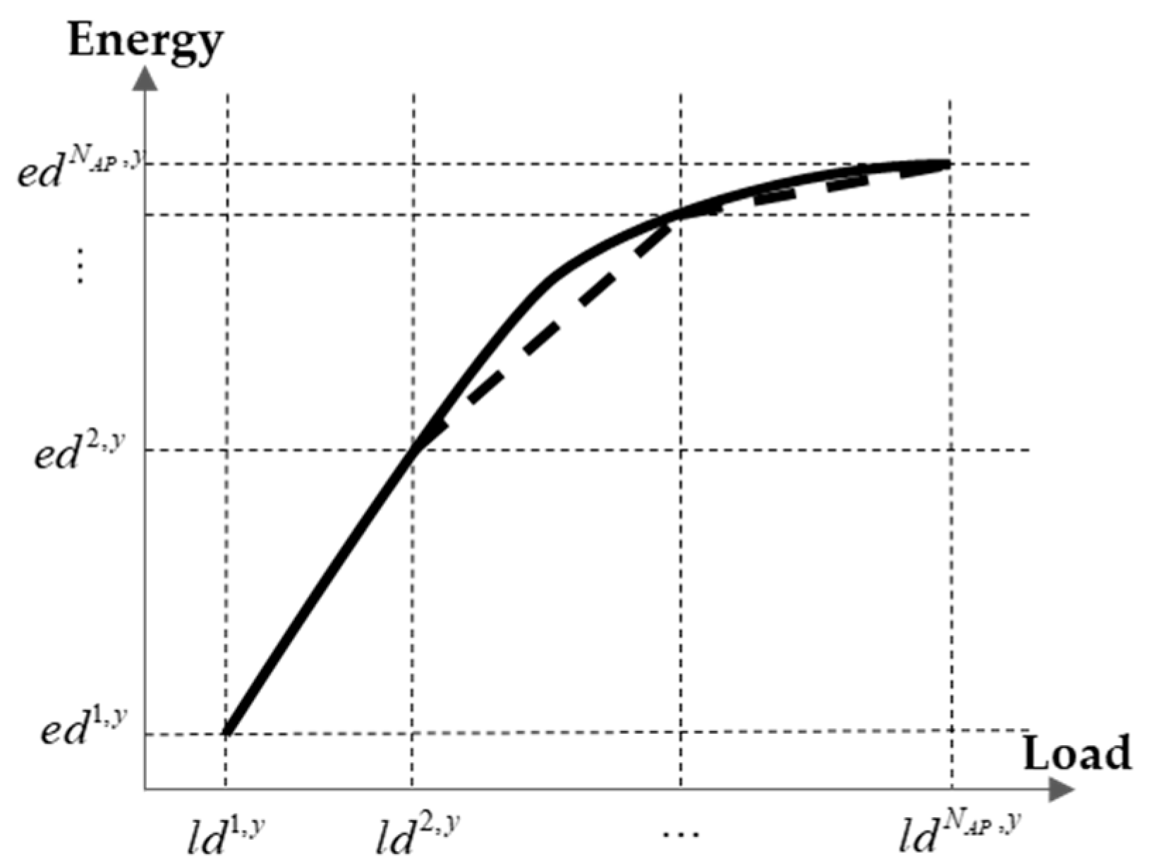
To appropriately model the MILP problem, the load-energy curve should be linearized. In this work, we apply the Douglas-Peucker algorithm to approximate this curve. This algorithm is used to reduce the number of points in a curve, which is defined as a series of points [30]. Moreover, it has been noted that applying this algorithm to the approximation of functions in the optimization problem improves the convergence of the optimization process, by simplifying the linear constraints [31]. Using this algorithm, the load-energy curve can be approximated precisely, even with a small number of straight lines, as shown in Figure 4. Here, the load-energy curve is depicted as a solid line, and the piecewise linear curve resulting from application of this algorithm is depicted as a dashed line. This algorithm constructs the piecewise linear curve by selecting $N_{AP}$ points on the load-energy curve.

4.2. Impact of the Renewable Electrical Power Source

In conventional expansion planning problems, the residual LDC (RLDC) is utilized instead of the LDC to analyze the impact of adopting a renewable electrical power source, which is treated as a negative load. The RLDC is formed by subtracting the chronological output pattern of the renewable electrical power source from the chronological load pattern and sorting this curve in descending order. To adopt the renewable electrical power source in the optimization process, the RLDC can be used. In our work, a residual load-energy curve should be constructed from the RLDC to analyze the renewable electrical power source, because the load-energy curve is used instead of the LDC.

The renewable electrical power source is no longer treated as a generation resource, because its generation amount is reflected in the residual load-energy curve. For this reason, the problem of deciding whether to adopt this resource is equivalent to choosing between the load-energy curve and the residual load-energy curve. If this resource is adopted, the residual load-energy curve is selected; otherwise, the load-energy curve is selected. The status of a candidate electrical load-energy curve is defined mathematically as:

$$u_{ELPAT}^{1,y}\ge 0,u_{ELPAT}^{2,y}={\displaystyle \sum _{i=1}^{N_{ER}}\left({\rho }_{RES,e}^i\cdot \left[{\displaystyle \sum _{si=1}^{N_{EST}}{u}_e^{i,si,y}}\right]\right)}\hspace{1em}\forall y.$$

(12)

The status of the candidate electrical load-energy curve denoted $u_{ELPAT}^{1,y}$ is 1 if the LDC is selected; otherwise the status denoted $u_{ELPAT}^{2,y}$ is 1. In addition, only one of the statuses of the candidate electrical load-energy curves can have a value of 1, as shown in Equation (13), since these curves cannot be selected at the same time in one project year:

$${\displaystyle \sum _{elp=1}^{N_{ELPAT}}{u}_{ELPAT}^{elp,y}}=1\hspace{1em}\forall y.$$

(13)

The operation cost of the renewable electrical power resource cannot be estimated in the same way as other resources, because the utilized energy of this resource is reflected using the residual load-energy curve. Hence, the total energy difference between the load-energy curve and the residual load-energy curve is treated as the utilized energy of this resource. This difference is reflected in the estimation of the operation cost of the renewable electrical power source, as follows:

$$\begin{array}{ll}{\mathrm{COST}}_{RES,e}^y& ={\displaystyle \sum _{i=1}^{N_{ER}}{\rho }_{RES,e}^i\cdot {\left(1+{\gamma }_d\right)}^{-y}\cdot \left(\left(CR{F}^i\cdot C{C}_e^i+FOM{C}_e^i\right)\cdot C_e^{i,1}\cdot \left[{\displaystyle \sum _{si=1}^{N_{EST}}{u}_e^{i,si,y}}\right]\right)}\\ & +{\displaystyle \sum _{i=1}^{N_{ER}}{\rho }_{RES,e}^i\cdot {\left(1+{\gamma }_d\right)}^{-y}\cdot \left(VOM{C}_e^i\cdot \left[\underset{eap\in EAP}{\max }\left(e{d}_e^{1,eap,y}\right)-\underset{eap\in EAP}{\max }\left(e{d}_e^{2,eap,y}\right)\right]\cdot \left[{\displaystyle \sum _{si=1}^{N_{EST}}{u}_e^{i,si,y}}\right]\right)}\end{array}.$$

(14)

Although the method for estimating fixed costs of this resource is similar to the method used for other resources, only a single candidate unit, $C_e^{i,1}$, is only used. This is because the RLDC depends on the output of a resource that varies with the capacity of the candidate unit.

The cost of the renewable electrical power source is not reflected in the total cost of electrical energy resources, as shown in Equation (2). Thus, the total cost of electrical energy should be modified considering the renewable electrical power source. Equation (15) defines the total cost including the modification. First, the cost of other resources is distinguished from the cost of the renewable energy resource by using the index, ${\rho }_{RES,e}^i$. Then, the cost of the renewable energy resource, as defined in Equation (14), is added to the total cost of the other resources as follows:

$$\begin{array}{cc}\hfill {\mathrm{COST}}_e^y=& {\displaystyle \sum _{i=1}^{N_{ER}}\left(1-{\rho }_{\mathrm{CHP},e}^i\right)\cdot \left(1-{\rho }_{RES,e}^i\right)\cdot {\left(1+{\gamma }_d\right)}^{-y}\cdot \left(CR{F}^i\cdot C{C}_e^i+FOM{C}_e^i\right)\cdot \left[{\displaystyle \sum _{c=1}^{N_C}{C}_e^{i,c}\cdot {\nu }_e^{i,c,y}}\right]}\hfill \\ & +{\displaystyle \sum _{i=1}^{N_{ER}}\left(1-{\rho }_{\mathrm{CHP},e}^i\right)\cdot \left(1-{\rho }_{RES,e}^i\right)\cdot {\left(1+{\gamma }_d\right)}^{-y}\cdot \left(F{C}_e^i+VOM{C}_e^i\right)\cdot \left[{\displaystyle \sum _{si=1}^{N_{EST}}{E}_e^{i,si,y}}\right]}+{\mathrm{COST}}_{RES,e}^y\hfill \end{array}\hspace{1em}\forall y.$$

(15)

Enough resources must be allocated in expansion planning such that the energy procured meets demand. Therefore, the total sum of the desired capacity and that of the utilized energy should be equal to, or over, the maximum load demand and the maximum energy demand, including the energy demand and the charging energy, respectively, as defined below:

$${\displaystyle \sum _{i=1}^{N_{ER}}{\displaystyle \sum _{si=1}^{N_{EST}}{P}_e^{i,si,y}}}\ge {\displaystyle \sum _{elp=1}^{N_{ELPAT}}\left(\underset{eap\in EAPS}{\max }\left(l{d}_e^{elp,eap,y}\right)\cdot u_{ELPAT}^{elp,y}\right)},{\displaystyle \sum _{j=1}^{N_{HR}}{\displaystyle \sum _{sj=1}^{N_{HST}}{P}_h^{j,sj,y}}}\ge \underset{hap\in HAPS}{\max }\left(l{d}_h^{hap,y}\right)\hspace{1em}\forall y$$

(16)

$$\begin{gathered} {\displaystyle \sum _{i=1}^{N_{ER}}{\displaystyle \sum _{si=1}^{N_{EST}}{E}_e^{i,si,y}}}\ge {\displaystyle \sum _{elp=1}^{N_{ELPAT}}\left(\underset{eap\in EAPS}{\max }\left(e{d}_e^{elp,eap,y}\right)\cdot u_{ELPAT}^{elp,y}\right)}+{\displaystyle \sum _{si=1}^{N_{EST}}{e}_{ESS}^{si,y}}\hspace{1em}\forall y, \\ {\displaystyle \sum _{j=1}^{N_{HR}}{\displaystyle \sum _{sj=1}^{N_{HST}}{E}_h^{j,sj,y}}}\ge \underset{hap\in HAPS}{\max }\left(e{d}_h^{hap,y}\right)+{\displaystyle \sum _{sj=1}^{N_{HST}}{e}_{TSS}^{sj,y}}\hspace{1em}\forall y. \end{gathered}$$

(17)

In expansion planning, the maximum load demand and energy demand can be changed by the statuses of the candidate electrical load patterns.

5. Optimization Process

5.1. Proposed Optimization Method

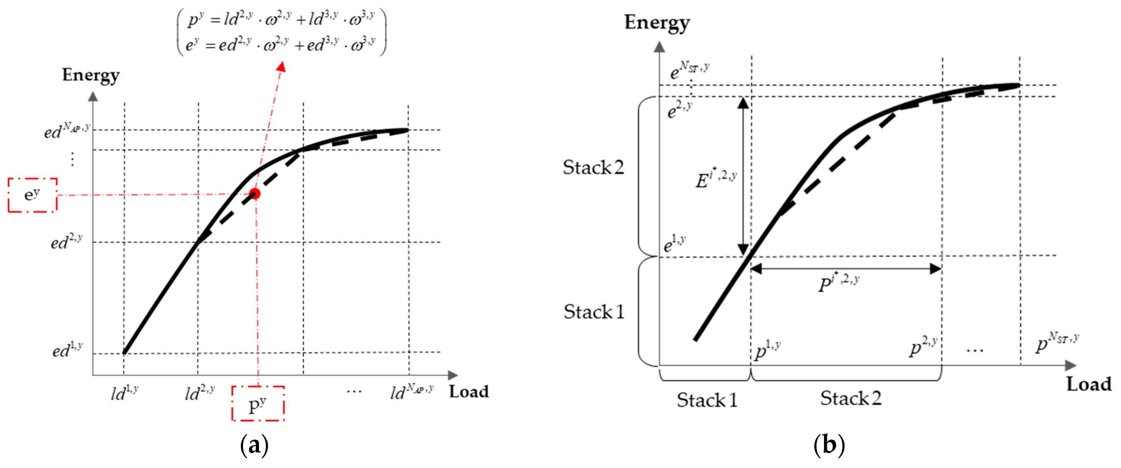
In our study, the installed capacity and the utilized energy of the energy resources are determined using a piecewise linear load-energy curve. For optimal allocation of the installed capacity and the utilized energy of the resources, a special ordered set of type 2 (SOS2) is used, which is known to be efficient for finding solutions to MILP problems [32]. Figure 5 illustrates the optimization process for determining a candidate resource. In the SOS2 method, as shown in Figure 5a, two adjacent SOS2 variables, ${\omega }^{2,y}$, ${\omega }^{3,y}$ ,are multiplied by the corresponding boundary node points to search for the desired load point, $p^y$, and energy point, $e^y$. After the desired points are located, the space, called a stack, between two adjacent desired points can be estimated and allocated to the candidate resource. Figure 5b depicts the desired capacity, $P^{2,y}$, and the utilized energy, $E^{2,y}$, determined using the stack between the two adjacent desired points. In the same way, $N_{ST}$ stacks can be configured, to allocate the resources.

Equations (18)–(24) detail the process for allocating the desired capacity and the utilized energy of the energy resources. In Equation (18), the value of the SOS2 variable is set to be less than the sum of the statuses of the two adjacent candidate segments:

$$\begin{gathered} {\omega }_e^{elp,si,eap,y}\le b{s}_e^{elp,si,eap-1,y}+b{s}_e^{elp,si,eap,y}\hspace{1em}\forall elp,\forall eap,\forall si,\forall y, (b{s}_e^{elp,si,0,y}=0) \\ {\omega }_h^{sj,hap,y}\le b{s}_h^{sj,hap-1,y}+b{s}_h^{sj,hap,y}\hspace{1em}\forall hap,\forall sj,\forall y, (b{s}_h^{sj,0,y}=0). \end{gathered}$$

(18)

According to the definition of the SOS2 method, the sum of two adjacent SOS2 variables must be 1, for one stack over one project year:

$${\displaystyle \sum _{eap=1}^{N_{EAP}}{\omega }_e^{elp,si,eap,y}}=u_{ELPAT}^{elp,y}, {\displaystyle \sum _{hap=1}^{N_{HAP}}{\omega }_h^{sj,hap,y}}=1\hspace{1em}\forall elp,\forall si,\forall sj,\forall y.$$

(19)

A candidate segment must be selected once, for one stack over one project year:

$${\displaystyle \sum _{eseg=1}^{N_{ESEG}}b{s}_e^{elp,si,eap,y}}=u_{ELPAT}^{elp,y}, {\displaystyle \sum _{hseg=1}^{N_{HSEG}}b{s}_h^{sj,hap,y}}=1\hspace{1em}\forall elp,\forall si,\forall sj,\forall y.$$

(20)

The desired point for determining the stack in the piecewise linear load-energy curve is estimated as follows:

$$p_e^{si,y}={\displaystyle \sum _{elp=1}^{N_{ELPAT}}{\displaystyle \sum _{eap=1}^{N_{EAP}}l{d}_e^{elp,eap,y}\cdot {\omega }_e^{elp,si,eap,y}}}, p_h^{sj,y}={\displaystyle \sum _{hap=1}^{N_{HAP}}l{d}_h^{hap,y}\cdot {\omega }_h^{sj,hap,y}}\hspace{1em}\forall si,\forall sj,\forall y$$

(21)

$$e_e^{si,y}={\displaystyle \sum _{elp=1}^{N_{ELPAT}}{\displaystyle \sum _{eap=1}^{N_{EAP}}e{d}_e^{elp,eap,y}\cdot {\omega }_e^{elp,si,eap,y}}}, e_h^{sj,y}={\displaystyle \sum _{hap=1}^{N_{HAP}}e{d}_h^{hap,y}\cdot {\omega }_h^{sj,hap,y}}\hspace{1em}\forall si,\forall sj,\forall y.$$

(22)

After determining the desired points, the desired capacity and the utilized energy are allocated by calculating the difference between the desired points as below:

$${\displaystyle \sum _{i=1}^{N_{ER}}{P}_e^{i,si,y}}=\{\begin{array}{cc}{p}_e^{si,y},& \mathrm{if}si=1\\ p_e^{si,y}-p_e^{si-1,y},& \mathrm{otherwise}\end{array}, {\displaystyle \sum _{j=1}^{N_{HR}}{P}_h^{j,sj,y}}=\{\begin{array}{cc}{p}_h^{sj,y},& \mathrm{if}sj=1\\ p_h^{sj,y}-p_h^{sj-1,y},& \mathrm{otherwise}\end{array}$$

(23)

$${\displaystyle \sum _{i=1}^{N_{ER}}{E}_e^{i,si,y}}=\{\begin{array}{cc}{e}_e^{si,y}+e_{EES}^{si,y},& \mathrm{if}si=1\\ e_e^{si,y}-e_e^{si-1,y}+e_{EES}^{si,y},& \mathrm{otherwise}\end{array},{\displaystyle \sum _{j=1}^{N_{HR}}{E}_h^{j,sj,y}}=\{\begin{array}{cc}{e}_h^{sj,y}+e_{TES}^{sj,y},& \mathrm{if}sj=1\\ e_h^{sj,y}-e_h^{sj-1,y}+e_{TES}^{sj,y},& \mathrm{otherwise}\end{array}.$$

(24)

Since the charging energy of the energy storage resources is not included in the load-energy curve, it is added to the utilized energy in Equation (24). The status of the candidate energy resource, $u_e^{i,si,y}$, $u_h^{j,sj,y}$, which is used for resource allocation of the stack, is defined as:

$$\begin{gathered} u_e^{i,si,y}=\{\begin{array}{rr}1,& \mathrm{if}si\mathrm{is}\mathrm{allocated}\mathrm{to}i\\ 0,& \mathrm{otherwise}\end{array}\hspace{1em}\forall i,\forall si,\forall y, \\ {u}_h^{j,sj,y}=\{\begin{array}{rr}1,& \mathrm{if}sj\mathrm{is}\mathrm{allocated}\mathrm{to}j\\ 0,& \mathrm{otherwise}\end{array}\hspace{1em}\forall j,\forall sj,\forall y. \end{gathered}$$

(25)

In Equations (26) and (27), the stack allocated to the candidate resource can be as large as the maximum capacity of the candidate unit of the specific resource. In these equations, the renewable electrical power source should be excepted since the output of this resource is reflected in the residual load-energy curve:

$$P_e^{i,si,y}\le \underset{c\in \mathrm{CANDIDATES}}{\max }\left(C_e^{i,c}\right)\cdot \left(1-{\rho }_{RES,e}^i\right)\cdot u_e^{i,si,y}, P_h^{j,sj,y}\le \underset{c\in \mathrm{CANDIDATES}}{\max }\left(C_h^{j,c}\right)\cdot u_h^{j,sj,y}$$

(26)

$$E_e^{i,si,y}\le \underset{c\in \mathrm{CANDIDATES}}{\max }\left(C_e^{i,c}\right)\cdot \left(1-{\rho }_{RES,e}^i\right)\cdot u_e^{i,si,y}\cdot 8760, E_h^{j,sj,y}\le \underset{c\in \mathrm{CANDIDATES}}{\max }\left(C_h^{j,c}\right)\cdot u_h^{j,sj,y}\cdot 8760.$$

(27)

In Equations (28) and (29), it is assumed that the stack is in charge of no more than one resource:

$${\displaystyle \sum _{i=1}^{N_{ER}}{u}_e^{i,si,y}}\le 1, {\displaystyle \sum _{j=1}^{N_{HR}}{u}_h^{j,sj,y}}\le 1\hspace{1em}\forall si,\forall sj,\forall y$$

(28)

$${\displaystyle \sum _{si=1}^{N_{EST}}{u}_e^{i,si,y}}\le 1, {\displaystyle \sum _{sj=1}^{N_{HST}}{u}_h^{j,sj,y}}\le 1\hspace{1em}\forall i,\forall j,\forall y.$$

(29)

The candidate unit of the resource should also be selected, because these units have different capacity. To select the candidate unit, the status of a candidate generating unit is designed as:

$$v_e^{i,c,y}=\{\begin{array}{rr}1,& \mathrm{if}c\mathrm{of}i\mathrm{is}\mathrm{chosen}\\ 0,& \mathrm{otherwise}\end{array}, v_h^{j,c,y}=\{\begin{array}{rr}1,& \mathrm{if}c\mathrm{of}j\mathrm{is}\mathrm{chosen}\\ 0,& \mathrm{otherwise}\end{array}\hspace{1em}\forall i,\forall j,\forall c,\forall y.$$

(30)

In addition, no more than one candidate unit should be selected, as shown in Equation (31), and the candidate unit should only be selected if any stack is allocated to the resource, as shown in Equation (32):

$${\displaystyle \sum _{c=1}^{N_C}{v}_e^{i,c,y}}\le 1, {\displaystyle \sum _{c=1}^{N_C}{v}_h^{j,c,y}}\le 1\hspace{1em}\forall i,\forall j,\forall y$$

(31)

$${\displaystyle \sum _{c=1}^{N_C}{v}_e^{i,c,y}}={\displaystyle \sum _{si=1}^{N_{EST}}{u}_e^{i,si,y}}, {\displaystyle \sum _{c=1}^{N_C}{v}_h^{j,c,y}}={\displaystyle \sum _{sj=1}^{N_{HST}}{u}_h^{j,sj,y}}\hspace{1em}\forall i,\forall j,\forall y.$$

(32)

In the previous process for allocating the resource, the maximum stack size is determined using Equations (26) and (27). However, these constraints are not sufficient for determining the desired capacity and the utilized energy, since the stack size is modified as the capacity of the candidate unit as follows:

$${\displaystyle \sum _{si=1}^{N_{EST}}{P}_e^{i,si,y}}\le \left(1-{\rho }_{RES,e}^i\right)\cdot \left[{\displaystyle \sum _{c=1}^{N_C}\left(C_e^{i,c}\cdot v_e^{i,c,y}\right)}\right], {\displaystyle \sum _{sj=1}^{N_{HST}}{P}_h^{j,sj,y}}\le {\displaystyle \sum _{c=1}^{N_C}{C}_h^{j,c}\cdot v_h^{j,c,y}}\hspace{1em}\forall i,\forall j,\forall y.$$

(33)

To remove the impact of the renewable electrical power source on resource allocation, it is excluded from the stack size constraint for electrical energy resources. The maximum utilized energy is defined by the capacity of the candidate unit of the resource as below:

$$\begin{gathered} {\displaystyle \sum _{si=1}^{N_{EST}}{E}_e^{i,si,y}}\le \left(1-{\rho }_{RES,e}^i\right)\cdot \left[{\displaystyle \sum _{c=1}^{N_C}\left(C_e^{i,c}\cdot v_e^{i,c,y}\right)}\right]\cdot 8760\hspace{1em}\forall i,\forall y \\ {\displaystyle \sum _{sj=1}^{N_{HST}}{E}_h^{j,sj,y}}\le \left[{\displaystyle \sum _{c=1}^{N_C}\left(C_h^{j,c}\cdot v_h^{j,c,y}\right)}\right]\cdot 8760\hspace{1em}\forall j,\forall y. \end{gathered}$$

(34)

5.2. Comparison of Optimization Results Using Different Load Curves

In this section, we examine the effectiveness of the proposed method with reference to a conventional method that uses a stepwise representation of the LDC. We compare the results of energy expansion planning for a single year using the non-linearized LDC, the stepwise representation of the LDC, and the piecewise linear load-energy curve. The objective of this problem is to minimize the total cost of the installed capacity and utilized energy of the two generators according to the cost data presented in

Table 1. Cost data for two generator units.

Unit	Fixed Cost ($/MW) (Capital Cost + Fixed Operations & Maintenance Cost)	Variable Cost ($/MWh) (Fuel Cost + Variable Operations & Maintenance Cost)
G1	60,000	100
G2	10,000	200

. For intuitive comparison of the results, we assume simplified cost data represented by the fixed cost and variable cost. On the basis of these data, G1 is expected to supply the majority of the load, whereas G2 supplies the shortfall of this load.

The load is assumed to be as depicted in Figure 6. Figure 6a shows the LDC, depicted using a solid line, and the stepwise representation of the LDC, depicted using a dashed line. The piecewise linear load-energy curve is illustrated in Figure 6b. The number of segments in the stepwise representation of the LDC is made equal to the number of segments in the piecewise linear load-energy curve. As shown in Figure 6, these curves are approximated by seven segments, such that the approximation error is less than 1%.

The results of the optimization performed using the data mentioned above are summarized in

Table 2. Results of the expansion planning problem.

Model No.	Type of Curve	Total Cost (M$)	Desired Capacity of G1 (MW)	Utilized Energy of G1 (GWh)	Desired Capacity of G2 (MW)	Utilized Energy of G2 (GWh)
0	LDC	858.9	1087.2	7885	126.0	19.9
1	Stepwise representation of LDC	866.8 (0.92%)	1028.8 (5.37%)	7780 (1.33%)	184.4 (46.35%)	126.1 (533.7%)
2	Piecewise linear load-energy curve	861.5 (0.31%)	1080 (0.66%)	7855 (0.38%)	133.2 (5.68%)	49.7 (150.3%)

. We define the models used to obtain the results as Model 0, where the non-linearized LDC was used; Model 1, where the stepwise representation of the LDC was used; and Model 2, where the piecewise linear load-energy curve was used. The results are listed according to the model, and the total cost, desired capacity, and utilized energy of the resources are compared. In this table, the errors in the results obtained using the approximated curves are estimated by comparison with the results of Model 0, and are expressed as percentages.

Overall, the results of Model 2 are better than those of Model 1. The error in total cost for Model 1 is 0.92%, which is 0.61% greater than the error for Model 2. The results for the desired capacity and utilized energy of G1 and G2 are more accurate when Model 2 is used than when Model 1 is used, as defined by their similarity to the results of Model 0. In particular, the error in the results for the desired capacity and utilized energy of G2 is more than three times larger with Model 1 than with Model 2. Therefore, it is better to use the piecewise linear load-energy curve to formulate the MILP problem than a stepwise representation of the LDC.

6. Case Study

In this section, we discuss the results of applying the proposed energy expansion planning method to an actual multi-energy system.

6.1. Data and Assumptions

We evaluated the proposed method using a comprehensive multi-energy system based on a benchmark determined by the energy system for Goyang city in Korea, which supplies electricity and heat with a 900 MW cogenerator. The cost parameters of the system are summarized in

Table 3. Cost parameters used in multi-energy system expansion planning.

Parameter	Value
Project lifetime (Year)	7
Interest rate (%)	3.91
Demand growth rate (%)	2.5
Approximation error tolerance (%)	1

.

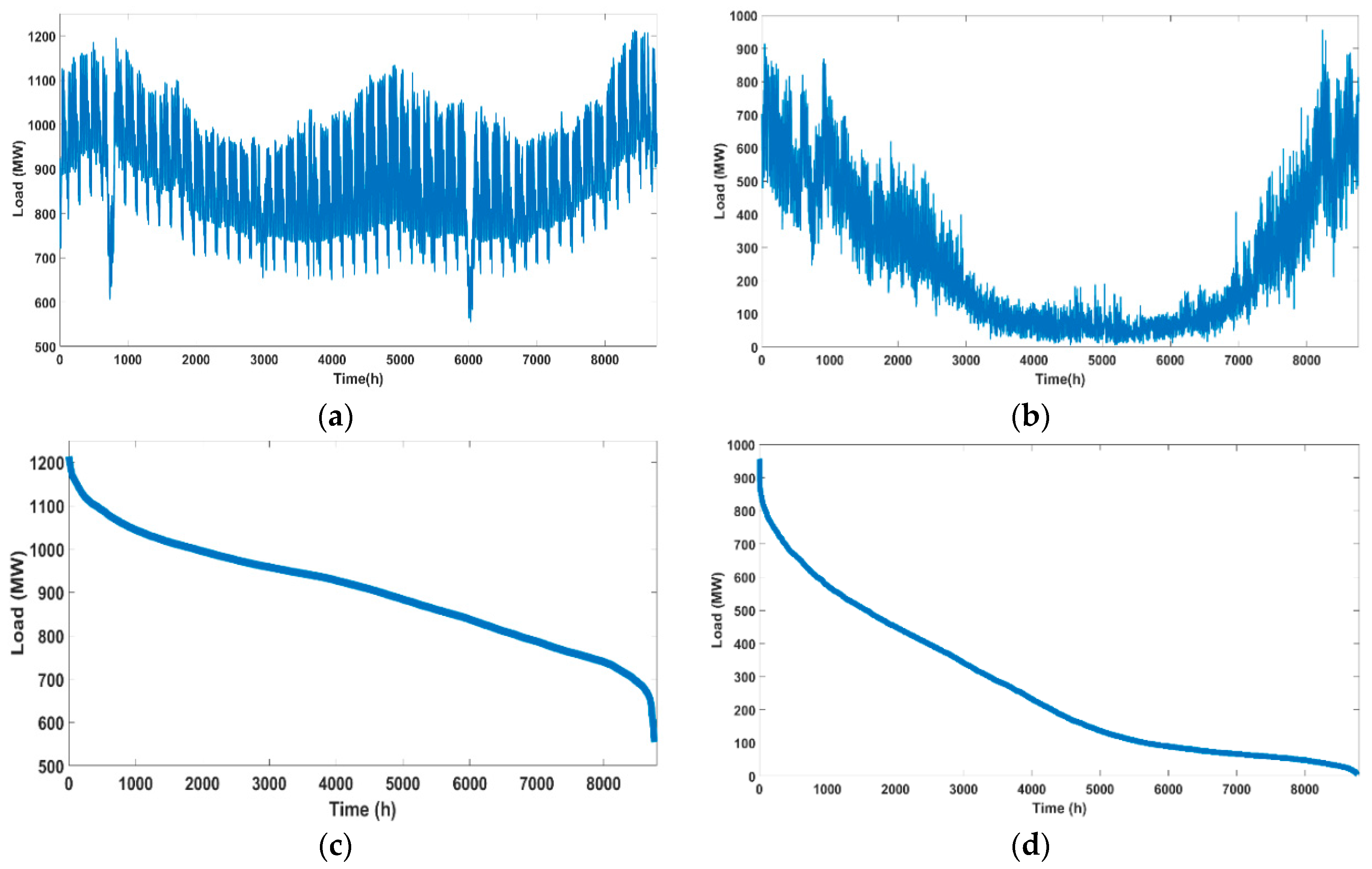
The project lifetime is assumed to be seven years, based on the lifespan of the electrical energy storage units [33]. The annual interest rate is considered to be 3.91% [34]. The rate of demand growth is assumed to be 2.5%, and the demand pattern is assumed to be the same each year. The approximation error tolerance of the Douglas-Peucker algorithm is 1%, to ensure accuracy, and reduce the computation burden, simultaneously. The energy load profiles are illustrated in Figure 7, where the heat load and electricity load profiles of the city are depicted in Figure 7a,b, respectively [35,36]. In addition, the LDCs for given loads are described in Figure 7c,d, respectively.

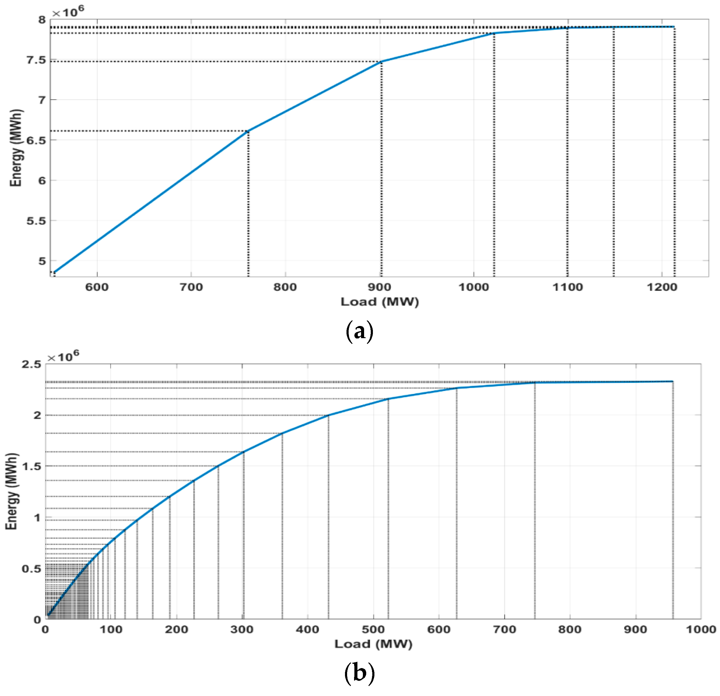
We constructed the load-energy curves for electricity and heat using these profiles, and linearized them using the Douglas-Peucker algorithm, as shown in Figure 8. As a result of the error tolerance of the Douglas-Peucker algorithm, defined in Table 3, there are 6 and 58 segments in the piecewise linear load-energy curve for electricity and heat, respectively.

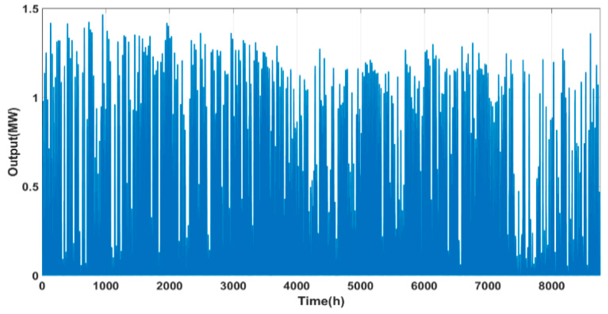
The renewable electrical power source is assumed to be a photovoltaic generator with a 13.3 MW capacity, where the output pattern for one year is as depicted in Figure 9 [37]. Using this pattern, the capacity factor of this resource was estimated below 11%.

Table 4. Energy resources data (O&M = operations and maintenance).

Resource Type	Unit Name	Overnight Capital Cost ($/MW)	Fixed O&M Cost ($/MW)	Fuel Cost ($/MWh)	Variable O&M Cost ($/MWh)	Life Span (Yr)	Candidate Capacity (MW)
Fuel-based Power Generator	DG1	900,000	15,000	33.2925	6.1	20	800, 700, 600, 500, 400, 300
	DG2	650,000	15,000	182.3	15	20	90, 80, 70, 60, 50, 40
	DG3	875,000	17,500	46.75	12.5	20	90, 80, 70, 60, 50, 40
Heat Only Boiler	HOB1	720,000	12,000	26.634	4.88	20	500, 450, 400, 350, 300, 250
	HOB2	520,000	15,000	182.3	15	20	400, 350, 300, 250, 200, 150
CHP	CHP	1,150,000	5850	22.77	2.75	20	900, 800, 700, 600, 500, 400 (Heat-to-Power ratio: 0.92)
Electrical Energy Storage	EES	3,092,000	42,000	0	35	7	24, 20, 16, 12, 8, 4
Thermal Energy Storage	TES	3,184,000	52,000	0	35	7	24, 20, 16, 12, 8, 4
Renewable Electrical Power Source	PV	1,375,000	10,500	0	0	20	13.3

shows the costs, life span, and candidate capacity of the candidate energy generation and energy storage resources used in this study. We defined the cost and life span of each resource as the average cost of the resource technology [33,38].

Among the technologies for energy generation resources, the multi-energy system would be expected to use gas-based and diesel-based resources, as these resources could be suitable for small-scale energy systems rather than bulk energy systems. Therefore, we assumed that the fuel-based power generators, DG1, DG2, and DG3, were based on a gas peaking, a diesel reciprocating, and a natural gas reciprocating engine generator, respectively. In addition, the heat-only boilers, HOB1 and HOB2, were assumed to be based on a gas boiler and a diesel boiler, respectively. Similarly, CHP was assumed to be based on a gas combined cycle. Further, the EES, TES, and PV were based on lithium ion battery energy storage, thermal energy storage, and solar photovoltaic generator, respectively. The candidate capacity of each resource was assumed according to the output capacity of multiple units, and the capacity of the CHP unit was defined on the basis of the performance of the 900 MW generator used in Goyang city. In addition, the heat-to-power ratio of the CHP unit was defined as 0.92.

6.2. Simulation Results

Table 5. Configurations of energy resources used in expansion planning.

Case Number	Fuel-Based Power Generator	Heat Only Boiler	CHP	Storage		Renewable Electrical Power Source
				Electrical Energy	Thermal Energy
1	◯	◯	◯	-	-	-
2	◯	◯	◯	◯	◯	-
3	◯	◯	◯	-	-	◯
4	◯	◯	◯	◯	◯	◯

shows four configurations of energy resources, defined so that the impact of adopting different combinations of energy resources could be analyzed. The fuel-based power generators, heat only boilers, and the CHP unit were included in all cases. To assess the impact of the other resources individually, the energy storage resources and renewable electrical power source were included in Case 2 and Case 3, respectively. Finally, in Case 4, we considered expansion planning using all the available resources.

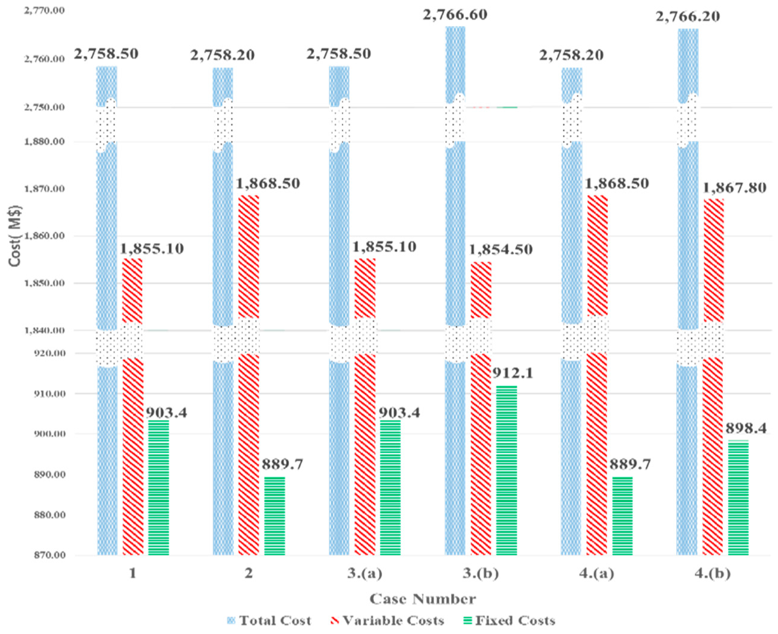
The proposed method was implemented in FICO Xpress and solved using standard branch-and-bound and simplex algorithms. The branch-and-bound algorithm was set to stop when a 0.1% duality gap was reached. The seven-year planning results for the four cases are presented in

Table 6. Seven-year planning schedules for Cases 1, 2, and 3 (RES = renewable electrical power source).

Year			1	2	3	4	5	6	7
Case No.	Forced Allocated of RES	Unit	Installed Capacity (MW)/Utilized Energy (GWh)
1	-	DG1	700/5553	700/5692	700/5834	700/5980	700/6110	700/6114	700/6118
		DG2	-	-	-	-	-	-	-
		DG3	-	-	-	-	40/18.83	40/168.3	40/321.5
		HOB1	250/152.3	250/155.7	250/159.3	250/162.9	250/166.7	250/170.5	250/174.4
		HOB2	250/9.488	250/10.062	250/10.65	250/11.25	250/11.87	250/12.51	250/13.16
		CHP *	700/2352(2164)	700/2411(2218)	700/2471(2273)	700/2533(2330)	700/2596(2388)	700/2661(2448)	700/2728(2509)
2	-	DG1	700/5553	700/5692	700/5840	700/6010	700/6110	700/6114	700/6118
		DG2	-	-	60/0.2462	60/0.7965	60/1.349	60/1.915	60/2.576
		DG3	-	-	-	-	50/75.33	50/252.1	50/417.8
		HOB1	300/155.0	300/158.4	300/167.5	300/192.8	300/220.7	300/249.4	300/263.0
		HOB2	250/6.792	250/7.366	250/8.264	250/9.619	250/11.01	250/12.43	250/15.63
		EES	-	-	-	-	-	-	-
		TES	-	-	-	-	-	-	8/14.08
		CHP *	600/2352(2164)	600/2411(2218)	600/2465(2267)	600/2502(2302)	600/2538(2335)	600/2575(2369)	600/2629(2418)
3	No	DG1	700/5553	700/5692	700/5834	700/5980	700/6110	700/6114	700/6118
		DG2	-	-	-	-	-	-	-
		DG3	-	-	-	-	40/18.83	40/168.3	40/321.5
		HOB1	250/152.3	250/155.7	250/159.3	250/162.9	250/166.7	250/170.5	250/174.4
		HOB2	250/9.488	250/10.062	250/10.65	250/11.25	250/11.87	250/12.51	250/13.16
		CHP *	700/2352(2164)	700/2411(2218)	700/2471(2273)	700/2533(2330)	700/2596(2388)	700/2661(2448)	700/2728(2509)
		PV	-	-	-	-	-	-	-
3	Yes	DG1	700/5551	700/5690	700/5832	700/5978	700/6110	700/6114	700/6118
		DG2	-	-	-	-	-	-	-
		DG3	-	-	-	-	40/16.78	40/166.2	40/319.4
		HOB1	250/152.3	250/155.7	250/159.3	250/162.9	250/166.7	250/170.5	300/177.1
		HOB2	250/9.49	250/10.06	250/10.65	250/11.25	250/11.87	250/12.51	200/10.46
		CHP *	700/2352(2164)	700/2411(2218)	700/2471(2273)	700/2533(2330)	700/2596(2388)	700/2661(2448)	700/2728(2509)
		PV	13.3/2.079	13.3/2.079	13.3/2.079	13.3/2.079	13.3/2.079	13.3/2.079	13.3/2.079

* CHP Shows Generated Electrical and Thermal Energy Together—Electrical Energy (Thermal Energy).

and

Table 7. Seven-year planning schedules for Case 4.

Year			1	2	3	4	5	6	7
Case No.	Forced Allocation of RES	Unit	Installed Capacity (MW)/Utilized Energy (GWh)
4	No	DG1	700/5553	700/5692	700/5840	700/6010	700/6110	700/6114	700/6118
		DG2	-	-	60/0.2462	60/0.7965	60/1.349	60/1.915	60/2.576
		DG3	-	-	-	-	50/75.33	50/252.1	50/417.8
		HOB1	300/155.0	300/158.4	300/167.5	300/192.8	300/220.7	300/249.4	300/263.0
		HOB2	250/6.792	250/7.366	250/8.264	250/9.619	250/11.01	250/12.43	250/15.63
		EES	-	-	-	-	-	-	-
		TES	-	-	-	-	-	-	8/14.08
		CHP *	600/2352(2164)	600/2411(2218)	600/2465(2267)	600/2502(2302)	600/2538(2335)	600/2575(2369)	600/2629(2418)
		PV	-	-	-	-	-	-	-
4	Yes	DG1	700/5551	700/5690	700/5838	700/6008	700/6110	700/6114	700/6118
		DG2	-	-	60/0.246	60/0.798	60/1.352	60/1.920	60/2.582
		DG3	-	-	-	-	50/73.24	50/250.0	50/415.7
		HOB1	300/155.0	300/158.4	300/167.5	300/192.8	300/220.7	300/249.4	300/263.0
		HOB2	250/6.793	250/7.367	250/8.264	250/9.619	250/11.01	250/12.43	250/15.63
		EES	-	-	-	-	-	-	-
		TES	-	-	-	-	-	-	8/14.08
		CHP *	600/2352(2164)	600/2411(2218)	600/2465(2267)	600/2502(2302)	600/2538(2335)	600/2575(2369)	600/2629(2418)
		PV	13.3/2.079	13.3/2.079	13.3/2.079	13.3/2.079	13.3/2.079	13.3/2.079	13.3/2.079

* CHP Shows Electrical and Thermal Energy Together—Electrical Energy (Thermal Energy).

. These tables show the planning schedule results, which describe the adopted resources, the capacity secured from each resource, and the amount of energy generated by each resource, over the project years. The cost-by-case results are shown in Figure 10. This figure shows the total cost, variable costs, and fixed costs, for each case. Note that the total cost of each case can be calculated by summing fixed costs and variable costs.

6.2.1. Case 1

In Case 1, we considered the impact of adopting fuel-based power generators, heat only boilers, and the CHP unit. The results of planning for this case, summarized in Table 6, show that DG1, HOB1, HOB2, and CHP are installed from the first project year, and DG3 is added in the fourth project year, because this resource is more expensive than DG1 and CHP. In addition, we note that the utilized electrical and heat energy of the CHP have a heat-to-power ratio of 0.92, matching the value defined in Table 3.

6.2.2. Case 2

In Case 2, we considered energy storage resources, in addition to the generation resources used in Case 1. We note that only TES is added from the available energy storage resources, as summarized in Table 6. Although the total cost and fixed costs are reduced by 0.01% ($0.3 × 10⁶) and 1.5% ($1.37 × 10⁷), respectively, variable costs increase by 0.72% ($1.34 × 10⁷). Compared to Case 1, the installed capacity of the CHP is reduced by 100 MW, and the utilized energy for the CHP is also reduced. However, resources such as DG2, DG3, and HOB1 are newly added, or extended, since the shortfall due to the reduction of the CHP should be secured. Although the utilizing electrical energy of DG3 is larger than that of DG2, the allocated capacity of DG2 is larger than that of DG3. DG2 delivers more energy at a cheaper variable cost than DG3. The installed capacity and the utilizing heat energy of HOB1 increase, because the installed capacity and the utilized energy of CHP are reduced. We note that TES, in the last project year, is charged from CHP, which has a relatively low variable cost.

6.2.3. Case 3

The renewable electrical power source was included for consideration in Case 3. However, the economic effectiveness of this resource is lower than the other resources, because its capacity factor is low. The schedule results in Table 6 show that, at the cost defined in Table 4, the renewable electrical power resource could not be allocated in the energy plan. Although allocating this resource is not necessary for creating an optimal plan, we tried to compulsorily force its adoption into the planning schedule, to validate its impact. For this reason, we considered two scenarios: one where this resource was forcibly allocated, and another when allocation was unrestricted. Comparing the difference between the two scenarios using Table 6, the utilized energy for DG3, which is the resource with the high variable cost, is reduced by 2.079 GWh, which is the utilized energy of PV, when PV is forced to be allocated. In the forcible allocation scenario, the utilized energy of DG1 is decreased in each year, between the first and the fourth project year, while between the fifth and the last project year, the utilized energy of DG3 is decreased. This suggests that allocating the renewable electrical power source reduces the utilized energy of resources with high variable costs. Due to this reduction, the variable costs in the forcibly allocated scenario are lower than that in the scenario when allocation is not forced, as seen in Figure 10. However, since PV is added in the forcible allocation scenario, the total cost and fixed costs are high.

6.2.4. Case 4

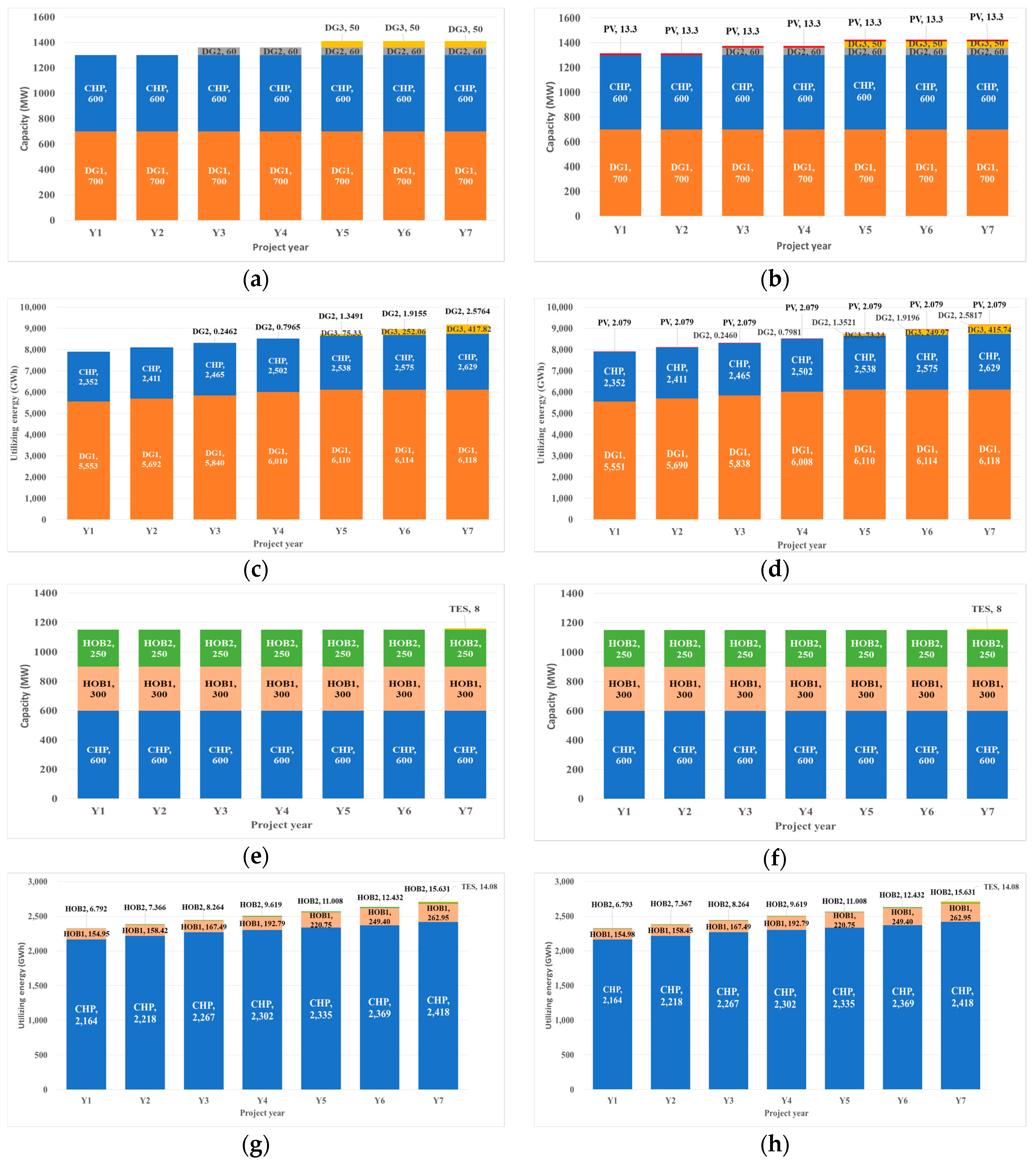
The energy storage resources and renewable electrical power source were included in Case 4. As with Case 3, this case is also divided into a scenario where the renewable electrical power source is forcibly allocated and one where allocation is unrestricted. As shown in Table 7, the renewable electrical power source reduces the utilized energy of the resource, which has a high variable cost. Between the first and fourth project years, the utilized energy of DG1 is decreased in the forcible allocation scenario. From the fifth to the last project years, the utilized energy of DG3 is decreased in the forcible allocation scenario. Although DG2, which has the highest variable cost, is installed in the third project year, its utilized energy is not decreased. This is because the utilized energy of DG3 is small compared to that of the PV, so the configuration of DG2 can be maintained without a reduction in energy. In terms of the use of energy storage resources, the planning schedule results are similar to those for Case 2, because the PV, with its lower capacity factor, does not change the results dramatically.

Figure 11 shows the results of the planning schedules described above graphically. Note that the energy resources are planned to meet the demand growth considering the presence or absence of forced allocation of RES. As in Case 3, the total cost of the scenario with forcible allocation is higher than that of the scenario where allocation is not forced. Compared to the forcible allocation scenario in Case 3, although the fixed costs are lower, the variable costs are higher, because the installed capacity of the CHP is decreased in this case, owing to utilization of the energy storage resource.

7. Conclusions

In this paper, we have proposed an optimization approach based on MILP, for expansion planning of a multi-energy system. The objective function of the problem was to minimize the total cost, composed of the investment and the operation cost of the electrical energy resources (including fuel-based power generators, an electrical energy storage, and a renewable electrical power source), the heat energy resources (including heat only boilers and a thermal energy storage), and the CHP unit, over the project years. To formulate the MILP problems, we used linearized load-energy curves instead of LDCs. With the load-energy curve, the energy demand used to calculate the cost of the resources can be utilized without the need for an integration operation, as is the case with the LDC. The Douglas-Peucker algorithm was used to linearly approximate the load-energy curve. The residual load-energy curve was used in defining the renewable electrical power source, for inclusion in the planning process. In the optimization process, the SOS2 approach was used to allocate the energy resources to meet the load and energy. A comparison of the proposed method using the load-energy curve with the conventional optimization method using the stepwise representation of the LDC demonstrated that the proposed method was better able to find the closest approximation to the desired solution, which was obtained by the non-linearized LDC, than the conventional method. We also compared different cases adopting different configurations of energy resources in a multi-energy system based on a benchmark determined using an actual energy system. The total cost and planning schedules were determined according to the cost and type of energy resources. The proposed method can help system operators of multi-energy systems design and optimize their model systems considering different energy resources, which are formulated as linearized constraints that can be easily used in commercial optimization software.

This study did not include an energy flow in which various energy sources can be converted and transferred to other sources. Thus, further studies in this field will focus on energy utilization in which energy sources can be integrated with and converted to other sources. In addition, although the operating region or the variable heat-to-power ratio should be considered in the actual operation of CHPs, the heat-to-power ratio for CHPs in this work was assumed to be constant. Therefore, in further studies, we will have to design linearized constraints that can take into account the actual operation of CHPs while maintaining the optimization model used in this study.

References

- Abdollahi, E.; Wang, H.; Rinne, S.; Lahdelma, R. In Optimization of energy production of a CHP plant with heat storage. In Proceedings of the 2014 IEEE Green Energy and Systems Conference (IGESC), Long Beach, CA, USA, 24 November 2014; pp. 30–34. [Google Scholar]
- Mancarella, P. MES (multi-energy systems): An overview of concepts and evaluation models. Energy 2014, 65, 1–17. [Google Scholar] [CrossRef]
- Shahidehpour, M.; Yong, F.; Wiedman, T. Impact of Natural Gas Infrastructure on Electric Power Systems. Proc. IEEE 2005, 93, 1042–1056. [Google Scholar] [CrossRef]
- Kalam, A.; King, A.; Moret, E.; Weerasinghe, U. Combined heat and power systems: Economic and policy barriers to growth. Chem. Cent. J. 2012, 6, S3. [Google Scholar] [CrossRef] [PubMed]
- Borelli, D.; Devia, F.; Lo Cascio, E.; Schenone, C.; Spoladore, A. Combined Production and Conversion of Energy in an Urban Integrated System. Energies 2016, 9, 817. [Google Scholar] [CrossRef]
- Lo Cascio, E.; Borelli, D.; Devia, F.; Schenone, C. Future distributed generation: An operational multi-objective optimization model for integrated small scale urban electrical, thermal and gas grids. Energy Convers. Manag. 2017, 143 (Suppl. C), 348–359. [Google Scholar] [CrossRef]
- Vandewalle, J.; Keyaerts, N.; Haeseleer, W.D. In The role of thermal storage and natural gas in a smart energy system. In Proceedings of the 2012 9th International Conference on the European Energy Market, Florence, Italy, 10–12 May 2012; pp. 1–9. [Google Scholar]
- Unsihuay-Vila, C.; Marangon-Lima, J.; de Souza, A.Z.; Perez-Arriaga, I.J.; Balestrassi, P.P. A model to long-term, multiarea, multistage, and integrated expansion planning of electricity and natural gas systems. IEEE Trans. Power Syst. 2010, 25, 1154–1168. [Google Scholar] [CrossRef]
- Chaudry, M.; Jenkins, N.; Qadrdan, M.; Wu, J. Combined gas and electricity network expansion planning. Appl. Energy 2014, 113, 1171–1187. [Google Scholar] [CrossRef]
- Moradi, M.H.; Hajinazari, M.; Jamasb, S.; Paripour, M. An energy management system (EMS) strategy for combined heat and power (CHP) systems based on a hybrid optimization method employing fuzzy programming. Energy 2013, 49, 86–101. [Google Scholar] [CrossRef]
- Salgado, F.; Pedrero, P. Short-term operation planning on cogeneration systems: A survey. Electr. Power Syst. Res. 2008, 78, 835–848. [Google Scholar] [CrossRef]
- Wouters, C.; Fraga, E.S.; James, A.M. An energy integrated, multi-microgrid, MILP (mixed-integer linear programming) approach for residential distributed energy system planning—A South Australian case-study. Energy 2015, 85 (Suppl. C), 30–44. [Google Scholar] [CrossRef]
- Geidl, M.; Koeppel, G.; Favre-Perrod, P.; Klockl, B.; Andersson, G.; Frohlich, K. Energy hubs for the future. IEEE Power Energy Mag. 2007, 5, 24–30. [Google Scholar] [CrossRef]
- Shahmohammadi, A.; Moradi-Dalvand, M.; Ghasemi, H.; Ghazizadeh, M.S. Optimal Design of Multicarrier Energy Systems Considering Reliability Constraints. IEEE Trans. Power Del. 2015, 30, 878–886. [Google Scholar] [CrossRef]
- Dzobo, O.; Xia, X. Optimal operation of smart multi-energy hub systems incorporating energy hub coordination and demand response strategy. J. Renew. Sustain. Energy 2017, 9, 045501. [Google Scholar] [CrossRef]
- Yu, S.; Zhang, S.; Sun, Y.; Tang, S. In Research on Interaction and Coupling of Various Energy Flows in Micro Energy Internets. In Proceedings of the 2017 IEEE International Conference on Energy Internet (ICEI), Beijing, China, 17–21 April 2017; pp. 53–58. [Google Scholar]
- Mozafari, Y.; Rosehart, W.; Zareipour, H. In Integrated electricity generation, CHPs, and boilers expansion planning: Alberta case study. In Proceedings of the 2015 IEEE Power & Energy Society General Meeting, Denver, CO, USA, 26–30 July 2015; pp. 1–5. [Google Scholar]
- Abbasi, A.R.; Seifi, A.R. Simultaneous Integrated stochastic electrical and thermal energy expansion planning. IET Gener. Transm. Distrib. 2014, 8, 1017–1027. [Google Scholar] [CrossRef]
- Abbasi, A.R.; Seifi, A.R. Unified electrical and thermal energy expansion planning with considering network reconfiguration. IET Gener. Transm. Distrib. 2015, 9, 592–601. [Google Scholar] [CrossRef]
- Ceseña, E.A.M.; Capuder, T.; Mancarella, P. Flexible Distributed Multienergy Generation System Expansion Planning Under Uncertainty. IEEE Trans. Smart Grid 2016, 7, 348–357. [Google Scholar] [CrossRef]
- Mojica, J.L.; Petersen, D.; Hansen, B.; Powell, K.M.; Hedengren, J.D. Optimal combined long-term facility design and short-term operational strategy for CHP capacity investments. Energy 2017, 118, 97–115. [Google Scholar] [CrossRef]
- Dolatabadi, A.; Mohammadi-ivatloo, B.; Abapour, M.; Tohidi, S. Optimal Stochastic Design of Wind Integrated Energy Hub. IEEE Trans. Ind. Informat. 2017, 13, 2379–2388. [Google Scholar] [CrossRef]
- Zhang, X.; Shahidehpour, M.; Alabdulwahab, A.; Abusorrah, A. Optimal Expansion Planning of Energy Hub With Multiple Energy Infrastructures. IEEE Trans. Smart Grid 2015, 6, 2302–2311. [Google Scholar] [CrossRef]
- Domínguez-Muñoz, F.; Cejudo-López, J.M.; Carrillo-Andrés, A.; Gallardo-Salazar, M. Selection of typical demand days for CHP optimization. Energy Build. 2011, 43, 3036–3043. [Google Scholar] [CrossRef]
- Zhou, X.; Guo, C.; Wang, Y.; Li, W. Optimal Expansion Co-Planning of Reconfigurable Electricity and Natural Gas Distribution Systems Incorporating Energy Hubs. Energies 2017, 10, 124. [Google Scholar] [CrossRef]
- Nastasi, B.; Lo Basso, G. Power-to-Gas integration in the Transition towards Future Urban Energy Systems. Int. J. Hydrog. Energy 2017, 42, 23933–23951. [Google Scholar] [CrossRef]
- Mathiesen, B.V.; Lund, H.; Connolly, D.; Wenzel, H.; Østergaard, P.A.; Möller, B.; Nielsen, S.; Ridjan, I.; Karnøe, P.; Sperling, K.; et al. Smart Energy Systems for coherent 100% renewable energy and transport solutions. Appl. Energy 2015, 145 (Suppl. C), 139–154. [Google Scholar] [CrossRef]
- Bakirtzis, G.A.; Biskas, P.N.; Chatziathanasiou, V. Generation Expansion Planning by MILP considering mid-term scheduling decisions. Electr. Power Syst. Res. 2012, 86, 98–112. [Google Scholar] [CrossRef]
- Li, J.; Li, Z.; Liu, F.; Ye, H.; Zhang, X.; Mei, S.; Chang, N. Robust Coordinated Transmission and Generation Expansion Planning Considering Ramping Requirements and Construction Periods. IEEE Trans. Power Syst. 2017, PP. [Google Scholar] [CrossRef]
- Douglas, D.H.; Peucker, T.K. Algorithms for the reduction of the number of points required to represent a digitized line or its caricature. Cartographica 1973, 10, 112–122. [Google Scholar] [CrossRef]
- Kolesnikov, A.; Fränti, P. Reduced-search dynamic programming for approximation of polygonal curves. Pattern Recognit. Lett. 2003, 24, 2243–2254. [Google Scholar] [CrossRef]
- De Farias, I.; Zhao, M.; Zhao, H. A special ordered set approach for optimizing a discontinuous separable piecewise linear function. Oper. Res. Lett. 2008, 36, 234–238. [Google Scholar] [CrossRef]
- Liu, Z.; Chen, Y.; Luo, Y.; Zhao, G.; Jin, X. Optimized Planning of Power Source Capacity in Microgrid, Considering Combinations of Energy Storage Devices. Appl. Sci. 2016, 6, 416. [Google Scholar] [CrossRef]
- Park, E.; Kwon, S.J. Solutions for optimizing renewable power generation systems at Kyung-Hee University‘s Global Campus, South Korea. Renew. Sustain. Energy Rev. 2016, 58, 439–449. [Google Scholar] [CrossRef]
- Korea-District-Heating-Coorperation (KDHC). Heat and Electricity Business Status. Available online: http://www.kdhc.co.kr/content.do?sgrp=S23&siteCmsCd=CM3655&topCmsCd=CM3715&cmsCd=CM4487&pnum=10&cnum=81 (accessed on 20 July 2017).
- Korea Power Exchange (KPX). Load Forecast. Available online: http://www.kpx.or.kr/www/contents.do?key=223 (accessed on 20 July 2017).
- Korea Farming and Fishing Village Construction. The Power Plant Generated Energy Present Condition for Photovoltaic Power Plants in Yeongam. Available online: http://www.data.go.kr/dataset/15005796/fileData.do (accessed on 23 July 2017).
- Lazard. Levelized Cost of Energy Analysis. Available online: http://www.lazard.com/perspective/levelized-cost-of-energy-analysis-100/ (accessed on 24 July 2017).
Figure 1.
Model of the multi-energy system.
Figure 2.
Illustrative LDC.
Figure 3.
Illustrative load-energy curve.
Figure 4.
Piecewise linear load-energy curve constructed using the Douglas-Peucker algorithm.
Figure 5.
Optimization process for determining the candidate resource: (a) Determining the desired point using the SOS2 method; (b) Allocating the capacity and utilized energy of a candidate resource.
Figure 6.
Load curves used in analysis: (a) LDC and stepwise representation of LDC; (b) Piecewise linear load-energy curve.
Figure 7.
Load profiles for the first project year: (a) Electricity load; (b) Heat load; (c) Load duration curve for electricity load; (d) Load duration curve for heat load.
Figure 8.
Piecewise linear load-energy curves for the first project year: (a) Electricity load; (b) Heat load.
Figure 9.
Output pattern of the renewable electrical power source.
Figure 10.
Estimated costs by case. (Note that, in the Case 3 and 4, (a) means a case with forced allocation of RES and (b) means a case without forced allocation of RES).
Figure 11.
Results of planning schedules for Case 4: (a) Installed capacity of electricity resources without forced allocation of RES; (b) Installed capacity of electricity resources with forced allocation of RES; (c) Utilized energy of electricity resources without forced allocation of RES; (d) Utilized energy of electricity resources with forced allocation of RES; (e) Installed capacity of heat resources without forced allocation of RES; (f) Installed capacity of heat resources with forced allocation of RES; (g) Utilized energy of heat resources without forced allocation of RES; (h) Utilized energy of heat resources with forced allocation of RES.