1. Introduction
The overall dispatching regulatory framework is experiencing a revision process in order to enable a more active participation by all energy resources (producers, consumers, prosumers) and the full exploitation of services by the Transmission System Operators (TSO)s and Distribution System Operators (DSO)s [
1,
2]. In this way, it will be possible to better exploit (economically) the services that can be provided even by the non-programmable resources, including those connected to the Medium Voltage (MV) and Low Voltage (LV) networks, traditionally excluded from the provision of ancillary services. The basic concept that should be underlined here is that such provision should be as much as possible independent from the traditional fossil fuel sources. Given the minimum requirements for the admission to the considered market session, the TSO should then select offers for ancillary services provisions that are based on economic merit and according to a criterion of technological neutrality [
3]. In this scenario, in order to evaluate if and to what extent it is reasonable to allow a dispatching service that involves production plants and final customers, it is quite important to analyze possible future assets of distribution networks. This will allow the active participation of producers to the electricity market, also enabling the Distributed Generation (DG) units connected to the LV and MV networks to supply balancing services. Moreover, in the future, the implementation of dispatching control in distribution networks will enable a more active participation also by final customers, promoting solutions for demand-side management and demand response.
The electrical system is evolving towards a smart grid system increasingly characterized by flexibility and interoperability [
4,
5]:
- -
from the point of view of thermal and hydropower producers that will be increasingly called upon to change their production profile to accommodate random generation sources;
- -
from the point of view of network operators, increasingly called upon to manage their networks actively involving subjects that until now were considered “not relevant” (rated size below 10 MVA);
- -
from the point of view of intermediaries (aggregators, market participants), increasingly called upon to play a more “technical” role, not only commercial, having to optimize the operation of production facilities in an integrated environment, taking into account the systemic needs;
- -
from the point of view of end users (LV consumers), those who are at the same time consumers and producers (prosumer), which will have to be increasingly involved in the context of demand-side management and demand response.
The aforementioned interoperability is not just about electricity producers, end customers and the respective network operators. It is also about the different network operators (there is an increasing need for close collaboration between TSOs and DSOs in relation to DG), and the different parties that are responsible for drawing up technical regulations that have to be increasingly integrated. What described so far shows a new electrical system that will take several years to be fully implemented but that has already started to operate.
The present work is part of the smart system landscape and, in particular, focuses on the active demand (AD) from the aggregation point of view of electrical loads in the form of LV users. Taking advantage of the flexibility in the consumption of participating users, this papers shows the key-role of loads clustering to create new energy resources that are able to operate in the electricity markets and in particular within the Ancillary Services Market (ASM) (the regulatory framework taken as background is the Italian energy market).
The aggregation of electrical loads is still a hot research topic and is treated by several important European projects among which the Address project (“Active Distribution networks with full integration of Demand and distributed energy resources”) [
6,
7,
8,
9], co-funded by the European Union in the 7th Framework Programme (2007–2013). The project was aiming to develop a comprehensive technical and commercial framework for the development of AD. According to Address, the new actor capable of performing the aggregation of electrical loads is called “Aggregator”, defined as an entity that collects, predicts, controls and manages a portfolio of distributed energy resources, in order to minimize the energy cost for “flexible” consumers (able to change their energy consumption) and maximize network injections from DG and AD. The Aggregator provides services to the actors of the energy system via the electricity market, brings interesting economic benefits for the consumers [
10] and environmental advantages for the community, supporting the development of renewable energy and thus reducing CO
2 emissions [
11,
12].
The main role of the Aggregator is to combine the loads’ flexibilities; in this way he is the mediator between consumers, of which sells the flexibility and the market, where such flexibility is sold to other participants in the energy system. For a satisfactory operation, the aggregator has to forecast the aggregated load demand response of a large number of prosumers, accordingly to various methods.
For example, in [
9] the authors propose a set of software tools for the aggregator, comprising short term forecasting of electricity market prices, forecasting of loads and their responses to control signals, optimal selection of the control signals and of the responses in each situation. In [
13] a simulation tool employing a bottom-up approach in order to build the aggregated load demand response model is described. Simulation of the individual responses is carried out with an optimization algorithm that minimizes the electricity bill whilst maintaining consumer’s comfort level. To improve the performance of the model, a genetic algorithm for fitting the input parameters according to measured data is also provided. In [
14] the authors propose a modelling and control protocol design approach for the aggregation of heterogeneous thermostatically controlled loads (TCL). The authors use a model predictive control scheme to obtain the optimal control actions along the prediction horizon. In addition, implementation of the control signal for adjusting TCLs’ statuses are also investigated with practical situations considered. In [
15] is presented a management approach that can be applied by an aggregator managing the flexibility of a large number of domestic electric storage water heaters. The approach aims at minimizing the electricity cost by using the thermal storage of the water heaters and is based on a model-free batch reinforcement-learning algorithm in combination with a market-based heuristic.
Differently from the above-cited research studies, in the present work a different connotation to the aggregation function is given. The main contribution of the work is the definition of a load aggregation system able to cluster end-users on the basis of their flexibility, in order to maximize the advantages of load aggregation in the ASM. In particular, the proposed system characterizes and classifies end-users by means of specific parameters, allowing to choose the most appropriate end-users for the provision of flexible services according to the needs of the grid.
The rest of the paper is organized as it follows:
Section 2, describes in detail the proposed system for end-users aggregation;
Section 3, describes the methodology used for load clustering;
Section 4, presents a case study showing the potentiality of clustering by means of the proposed system;
Section 5, finally, contains the conclusions of the paper.
2. Monitoring System and Web Platform for Bottom-Up Aggregation
The choice of customer baseline is fundamental in demand response (DR) markets [
16]. From the electrical user side, offering a flexible service means meeting the requests from the manager of the ASM within one hour, by means of the variation of its electric “habits”. This change of habits, in terms of average hourly power consumption, is highly dependent on the following aspects: types of appliances present at the user’s facility, electric habits, ability to change habits. The three points mentioned are different but at the same time highly correlated [
17,
18,
19,
20]. In the proposed system, the single user determines the priorities of electrical appliances, choosing voluntarily, and in relation to a certain time period.
Based on these considerations, it is possible to give the definition of flexibility as actually intended in this work: “average hourly power that a given user can provide, upwards (f_up) or downwards (f_down) or both, compared to the average hourly power (Pm) absorbed under normal conditions”.
According to the above definition, being Pm the average power requested by the user in a given hour, the flexibility is intended as the quota of power sf (f_up or f_down) that the user can sum or subtract to Pm for participating to the ancillary service market. As a consequence, the user is characterized in a specific hour by:
Pm, the average power absorbed when the end user does not take part to the ancillary service market;
sf, the flexibility of the user;
Pmf = Pm + sf, the average power the user can absorb when participating to the ancillary service provision.
Other definitions of flexibility have been given over time, the most recent ones [
21,
22] based on statistical considerations that assess the ability of groups of users to change their consumption in specific future periods of time. The study carried out here, however, does not rely on a statistical approach. Indeed, the parameters chosen for the characterization of the individual user, together with continuous learning ability about consumer behavior implemented in the platform, allow to classify and always select the users deemed best to participate in the creation of new energy resources, in a specified timeframe.
Therefore, according to the above definition of flexibility, to evaluate the flexibility of each user in the considered hour it is essential to determine the average power
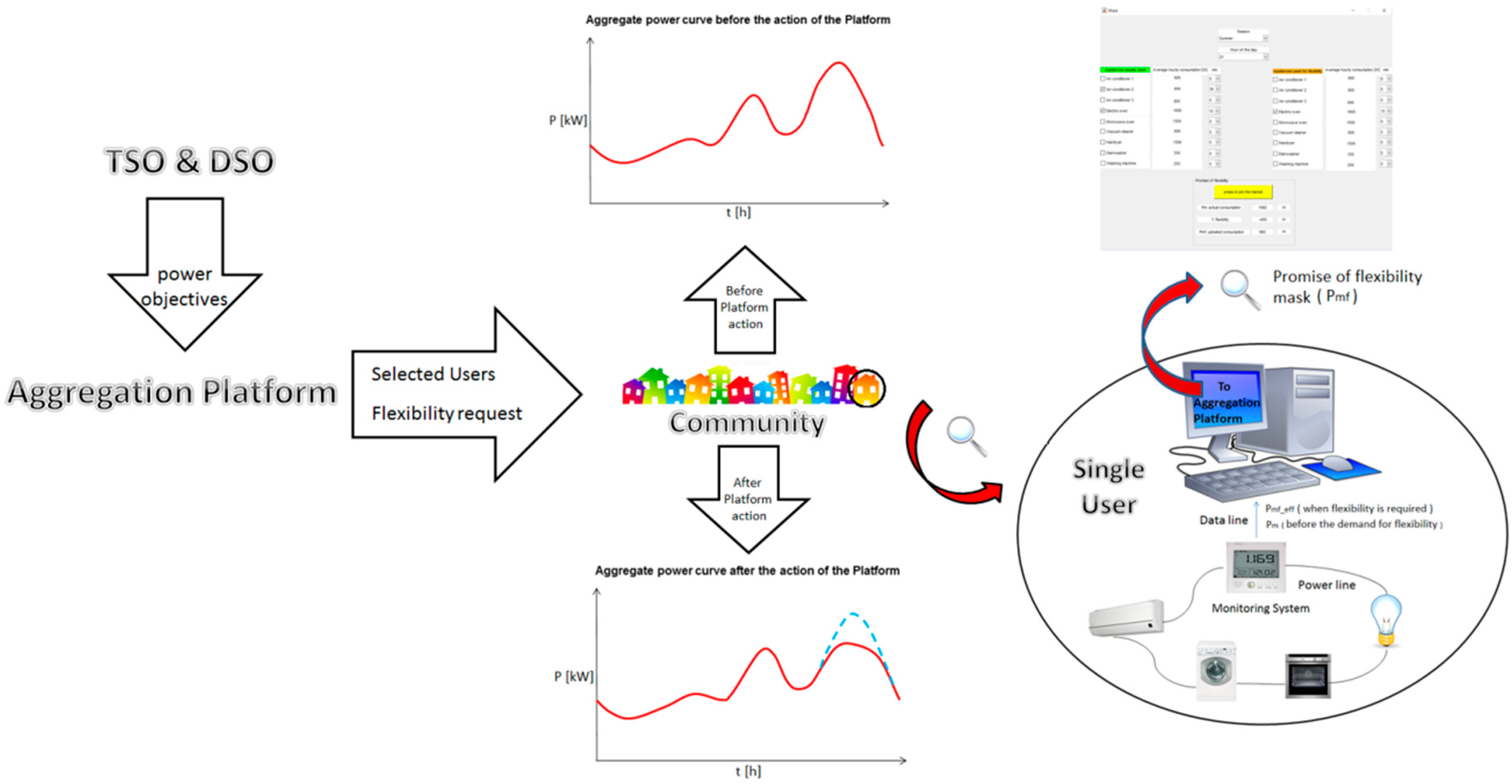
Pm. This is done by using a suitable monitoring system, installed at the user’s premises, able to record the hourly average power and connected to a web platform enabling the participation of the user at the ancillary service market (
Figure 1).
In a realistic scenario, the monitoring system could be provided by the electrical utility supplying the community of end-users, given that it is the party that has the main advantages from the exploitation of the users’ flexibility.
In
Figure 1, the aggregation platform receives a flexibility request by the DSO/TSO and sends it to the community of end-users. Each user, for every hour of the day offers its flexibility by entering the web platform.
Initially, each user, once signed up on the load aggregation web platform, must necessarily go through an initializing period in which its consumption is monitored precisely. From this first phase of monitoring, a vector Pms,d is defined that, for a generic user contains the average power values and is made of 4 (seasons) × 2 (typical days) × 24 (hours) elements:
where s is the season (four seasons: summer, winter, fall, spring) and d is the day (two typical types of days: weekdays and holidays). For simplicity, in the following the subscripts s and d will not be reported. The user can set the system in order to characterize more than two typical days, according to its personal habits. Therefore, vector Pms,d can contain more than 4 × 2 × 24 elements.
This first phase of consumption characterization is only one of the two basic actions that the monitoring system is expected to perform. In fact, a second phase, that is equally important, is the one relating to the monitoring of the average hourly consumption of each user, after that it has been required to exert a certain flexibility. Ultimately, the monitoring system has to play two equally essential actions:
Phase 1: user monitoring from the time of subscription to the platform, so as to record the daily consumption and make a first classification;
Phase 2: continuous monitoring in order to verify compliance with the declaration of user flexibility.
Phase 2 is considered fundamental in the determination of the relative flexibility parameter; the features described above, namely the average power value of absorbed power without flexibility and the flexibility, are not able to give a full characterization of the user. Indeed, it is necessary to define another key parameter for the classification of the users. This parameter is called relative flexibility (a) and takes into account the actual behavior of each user with respect to the flexibility that the same customer declares:
where Pmf_eff is the hourly average power actually absorbed by the user after the request of a given flexibility.
The relative flexibility parameter takes into account the user’s behavior in a certain time (a day, a season, etc.). In order to achieve a correct characterization of each user, this parameter must be calculated as the average of many “a” parameters, calculated as described above in equivalent homogeneous hours (hours belonging to the same day and season). By implementing this method, the relative flexibility holds memory of past behavior and the greater the number of averaged parameters, the better the characterization of the users. Another important aspect to consider is the treatment of any extraordinary behavior of the individual user. From this point of view, the authors found correct to eliminate the highest and the lowest registrations. Ultimately, the characterization of the individual user is made on the basis of two quantities that must, for a certain time, be necessarily associated with each user:
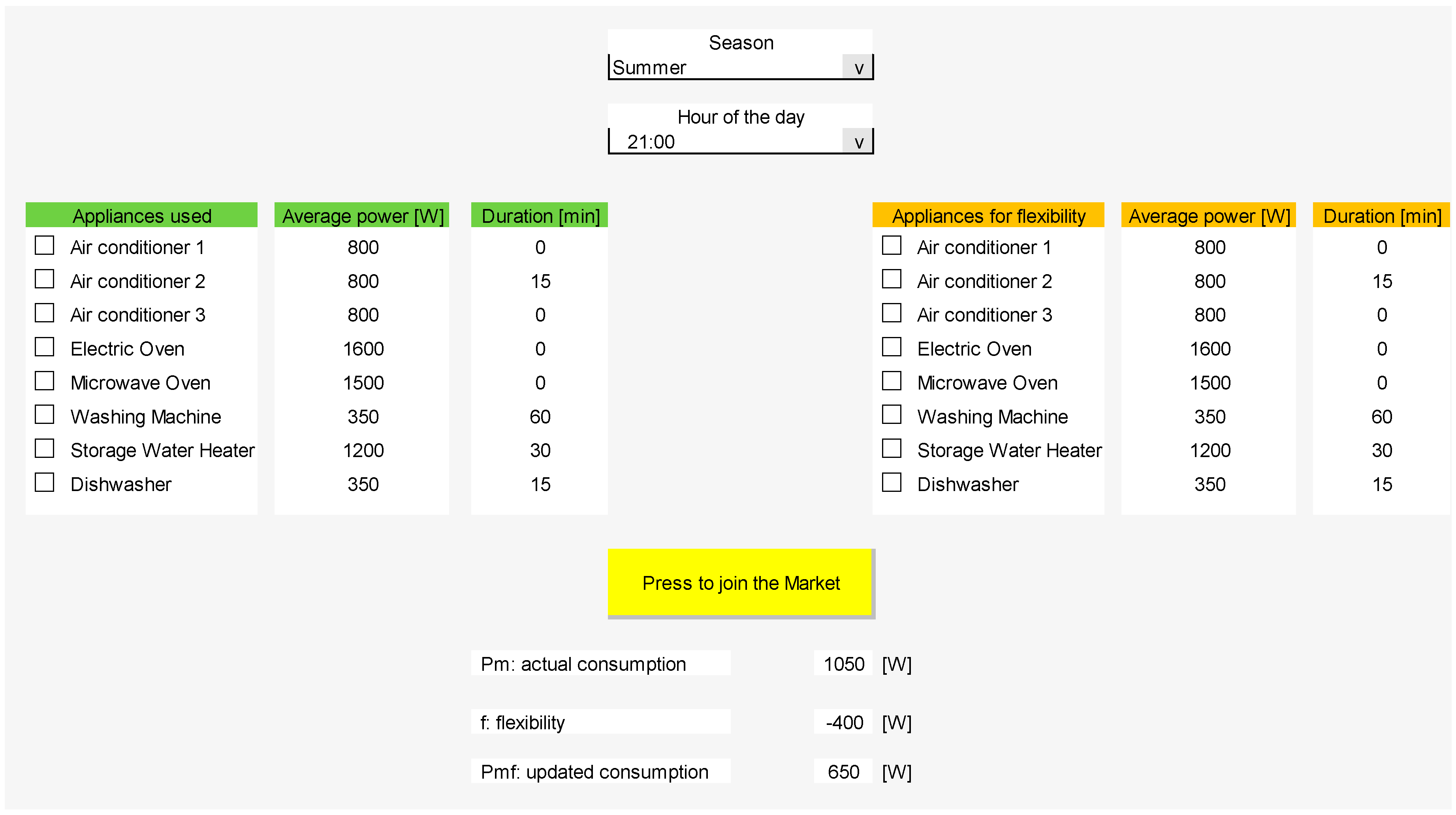
Most of the commercially available apparatus for domestic load monitoring easily allow the registration of the energy absorbed by each appliance in a given timeframe. Some of these tools allow the wireless transmission of the data to a local concentrator, where further elaborations can be carried out. To evaluate precisely the flexible power of each appliance and thus the flexibility offer that the user can display at given hour of the day, any of these commercial monitoring apparatus are needed. The load aggregation platform must take into account that the users, in most cases, are managed by non-expert people that may not know how to translate a given demand of flexibility (expressed in Watt) in terms of use of a given appliance. In this aim, a Matlab code was designed to determine for each hour of the day what combination of appliances, and for how long, can be used to satisfy a given flexibility requirement. The same software is used to support the user to formulate his own flexibility proposal at a given hour, using a drop down menu in the user interface (
Figure 2), even before the same user is asked to display a given amount of flexible power.
The proposal about flexibility must be displayed by the user before the algorithm defines the participant users and their degree of flexibility (contribution that must be compatible with the flexibility declared by each user). Flexibility can be upwards or downwards. The software can include a safety coefficients for lowering the error that each end user can do in the evaluation of its own flexibility.
Summarizing, the single user’s code is composed of two parts:
the first part helps the user to compose the flexibility offer in the platform starting from the possibility to shift in time the appliances use;
the second part helps the user to choose the appliances to be used to satisfy the flexibility demand coming from the aggregation platform and to formulate the final flexibility offer.
This last part of code is structured so as to combine different appliances (up to four); if only one appliance can satisfy the request, the algorithm can display the correct operating or non operating time. The time interval in which the aggregation algorithm displays its functions is one hour, since from one hour to the next, the users can be clustered differently and the needs of the ASM may change. The main functions of the platforms are:
acquiring data from the market;
acquiring data from users;
clustering users;
conceiving and producing composite offers of flexibility on the ASM.
The energy needs of the ASM, defined by the TSO and DSO, are translated and sent to the aggregation platform through two hourly average power values, once defined the objectives of powers:
hourly average power Pobb, to which each user must as much as possible comply by means of the declared flexibility;
hourly average power Ptot, the platform asks the aggregate of users as a consequence of the ASM needs.
The first value is needed to create a clear objective for each user that will be satisfied acting on the local flexibility. Moreover, the software can employ different types of flexibility according to the type of appliance considered. The latter may indeed have an on-off or modulating behavior. Based on the flexibility declared by each user, two extreme behaviors can be identified:
users that at that time offer large flexibility and that are thus available for varying their electric ‘habits’ in order to offer a service to the electrical system;
users that can or cannot vary their own consumptions and do not have a high flexibility, namely availability of flexible power.
3. Users Clustering
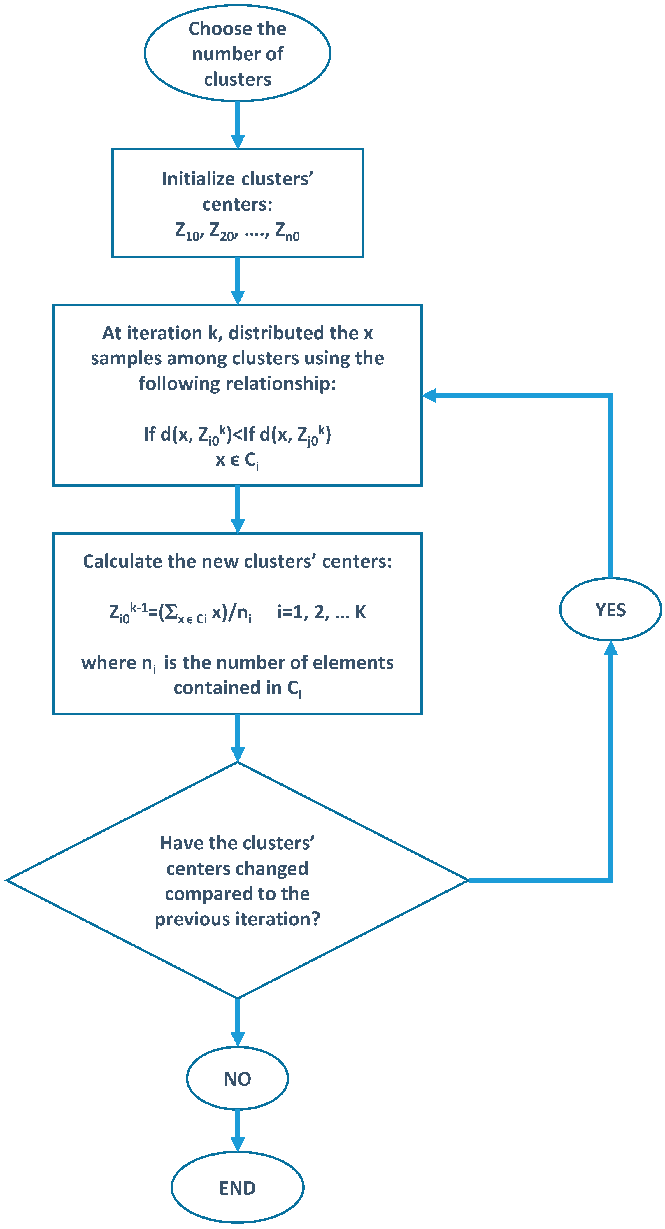
The method used for users clustering is the well-known
k-means algorithm [
23], “
k” being the number of clusters identified in the group of users (
Figure 3).
The algorithm can classify a given number of objects in k smaller subgroups. The clustering takes place by minimizing the sum of Euclidean distances between the elements and the reference cluster center. Such minimization is carried out in an iterative and heuristic way, depicted in
Figure 3 below and explained in the following lines. Variables of the optimization are the clusters composition:
where:
E is the function to be minimized;
Ci is the i-th cluster;
Zi is the coordinate of the center of cluster Ci;
is the Euclidean distance between a point x and Zi, the coordinate of the cluster center.
Here the minimization is intended as the way to find the best classification of samples into subgroups. So, at each iteration, a new classification is tested and new cluster centers are identified. In this way, as a new clustering is considered, each element is assigned to the cluster for which the distance to the cluster center is reduced as compared to the current choice.
The
k-means clustering algorithm [
24,
25] is not a global optimization method, although it proved to provide good solutions whose quality depends largely on the quality of initial choice of cluster centers. The variables are the clusters identified, namely the attribution of a class to each sample.
The algorithm is described by the flow chart in
Figure 3 and comprises the following steps:
- (1)
choice of the number of clusters;
- (2)
preliminary calculation of the clusters’ centres;
- (3)
distribution of the users between clusters;
- (4)
calculation of the new centres’ coordinates.
The algorithm repeats steps 3 and 4 until the cluster centers’ coordinates do not vary.
The clustering module is a simple tool that is extremely efficient if the clustering parameters contain useful information for the aim of providing good coverage of the demand from the ASM. It works also with thousands of elements providing a solution in a very short-time.
Following the logic of the implemented algorithm, the clustering cannot neglect two parameters that are considered very relevant:
- (1)
the absolute difference, between the target value P
obb and the average hourly power the user declares to be able to absorb by means of its own flexibility:
- (2)
the absolute difference between the relative flexibility and 1 (ideal relative flexibility).
The first classification parameter gives evidence of the declared capacity of each user to satisfy the average hourly power. The second gives evidence of the actual fulfillment of the promised flexibility by each user.
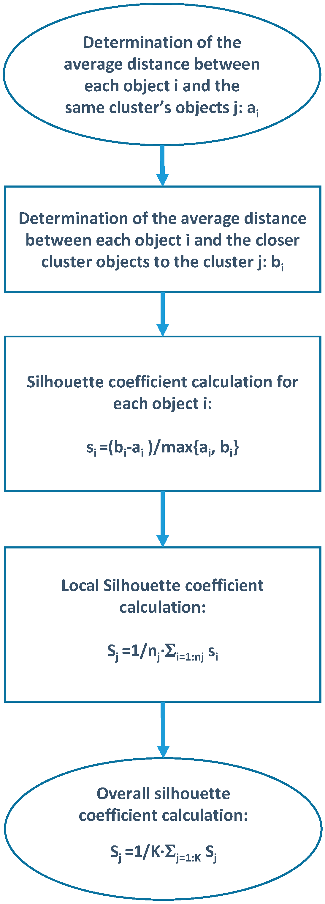
It is evident how the groups depend on the initial chosen cluster centers and also by the number of clusters k. The validation of the k-means algorithm is the main subject of validity of the clustering. Different approaches exist to execute the validation of the algorithm. One of the most common is the one based on the “
Silhouette global index” (SC) [
26] determination.
Figure 4 shows the flow chart of the validation algorithm for the k-means algorithm results. As it can be observed, the validation algorithm comprises four steps:
- (1)
evaluation of the average distance ai between each object i and the other objects j belonging to the same cluster;
- (2)
evaluation of the average distance b between each object i and the objects j belonging to the closer cluster;
- (3)
calculation of the silhouette coefficient for each object;
- (4)
calculation of the local silhouette coefficient;
- (5)
calculation of the overall silhouette coefficient.
Studies carried out over the validation process [
27] have brought the following indication for the assessment of the global
Silhouette coefficient:
0.71–1 → strong structure;
0.51–0.7 → medium structure;
0.26–0.5 → weak structure;
<0.25 → no substantial structure.
Based on this interpretation, the implemented algorithm is able to identify the optimal number of clusters, among those allowed (2 < k < , where n is the number of users to be classified), in which the platform users can be classified).
At the basis of the choice of the users called to respond to power requirements, as well as the classification made, there is the further need to order the elements belonging to each cluster in relation to their relative flexibility. This need arises from the fact that, if to meet the total requirement of average power Ptot, is not necessary to select all the elements of a given cluster, it is good that in this said selection the most “reliable” (those with smaller absolute value difference, relative to unitary flexibility) take part.
The ultimate goal is the choice of the users according to the order defined above and the determination of the flexibility each user can implement, in relation to its declared flexibility and to the own relative flexibility. In this phase, the relative flexibility of each user is used by the code to take into account the actual behavior of each user. This is done by multiplying the elements of flexibility to go up and down (vectors with as many elements as many users, containing the declared flexible power availability) for the respective values of relative flexibility:
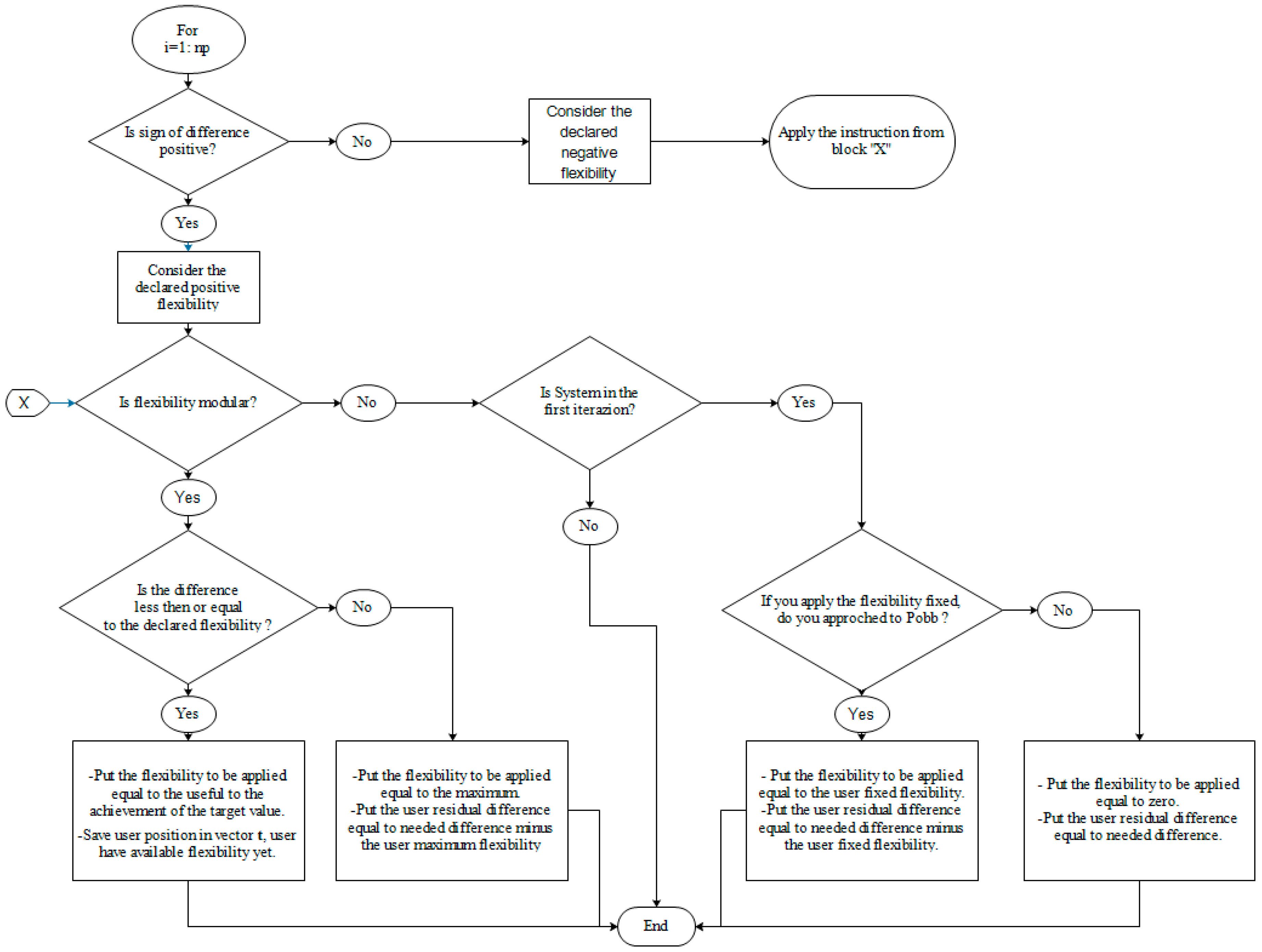
The algorithm created for performing the actions described consists of a series of nested loops. The outer loop is a while loop, whose stop condition is one for which the total average power obtained by means of the aggregation of users (sumP) must be limited within a certain interval around the target value of the total average power Ptot. This range is around ±2%.
Another variable to be initialized is the number of users chosen for the load aggregation np. Such a number:
Within the above described loop, an internal while loop executes instructions until the convergence is reached with the considered number of users, np.
The convergence is reached when the power difference the users must implement through their own flexibility capability does not change in two subsequent iterations. The instructions contained in the second while cycle, having the aim of determining the power differences that each user must apply by means of its own flexibility, are reported in
Figure 5.
4. Application
In this section, are shown and commented the results of the application carried out for a realistically simulated set of customers. Considering a typical community of residential end-users supplied by the same substation, 100 customers are considered. These results are referred to set of input data and strictly depend of the values of the vectors a, f_up (f_up(1), f_plus(2)… ) ed f_down (f_down(1), f_down(2)… ), calculated in random mode but coherently with the same input data (power Pm).
4.1. Input Parameters of the Algorithm
In the application, a sample of 100 homogeneous domestic users has been chosen. The sample has been outputted using the simulator developed in [
28] and based on a Monte Carlo approach and real usage probability data for domestic devices and appliances. For each of them the vector Pm has been defined. The time period between 8 p.m. and 9 p.m. in a summer holiday has been chosen. The following target values for power has been assumed:
In
Table 1, the input vectors for the clustering algorithm are reported. The vectors
a_1 and
a_2 represent two different conditions:
a_1 is the input for which users showing very different habits, with different degrees of reliability (very different “a” parameters), are considered;
a_2 is the input for which users showing similar habits are considered. Values in the vector are close to unity (users with similar behavior and reliable in terms of fulfillment of promised flexibility).
In particular, a_1 contains values that are dispersed in a large interval, as for example 0.1–1.9, while a_2 contains the same number of values, in a smaller range, as 0.51–1.44 (with a greater concentration around the unity). This discrimination comes from the need to show how the algorithm works in presence of different clusters of users.
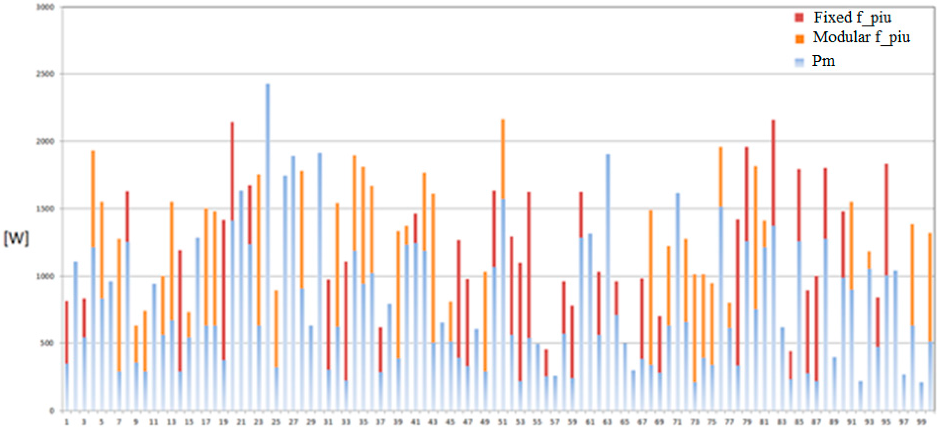
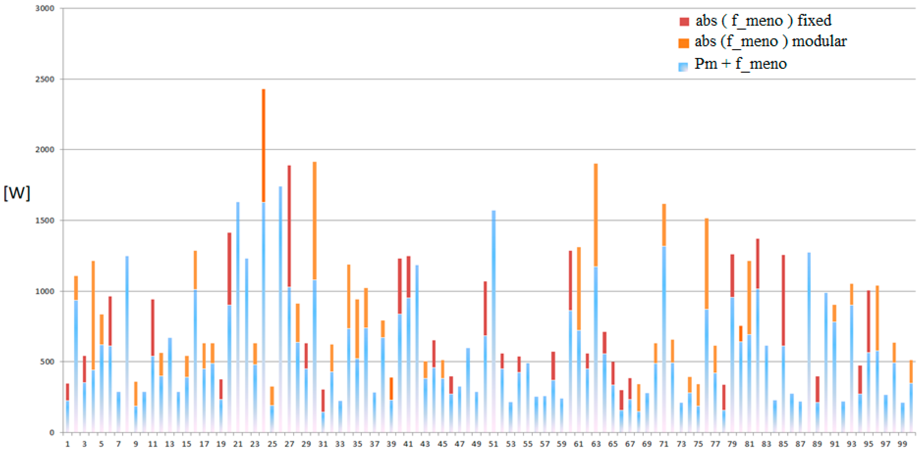
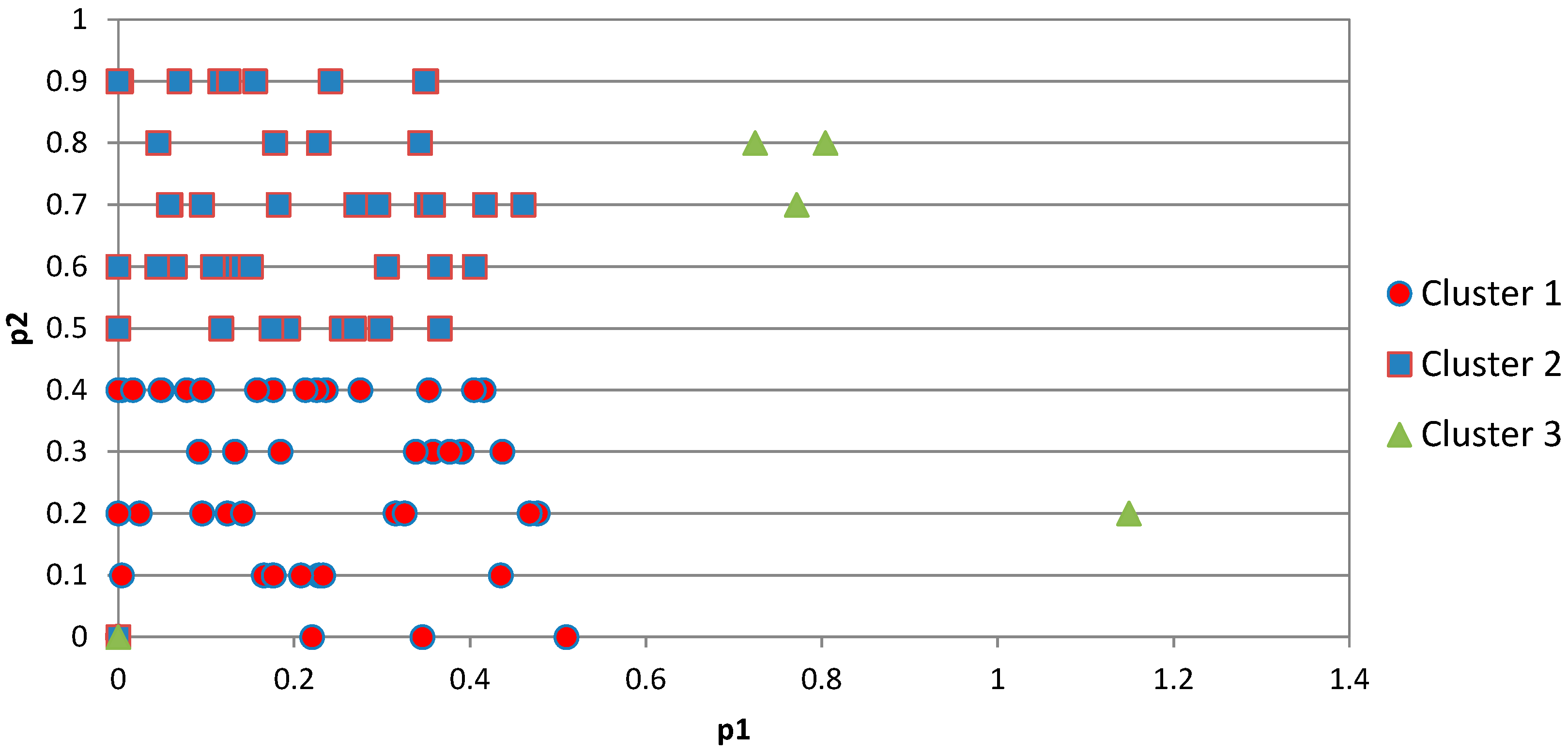
Figure 6 and
Figure 7 are a graphical representation of the declarations about flexible powers of each user, also keeping into account the further discrimination about the possibility to modulate the promise of flexibility.
4.2. Results of the Clustering and Choice of Users to Satisfy the Demand
In this section, the results of
k-means clustering based on parameters 1 and 2 previously defined are reported. As already expressed above, to show the effect of clustering in different conditions, the classification parameter 2 is first chosen, using the two relative flexibility vectors
a_1 (case 1) and
a_2 (case 2) reported in
Table 2 and
Table 3, respectively.
4.2.1. Results Analysis—Case 1
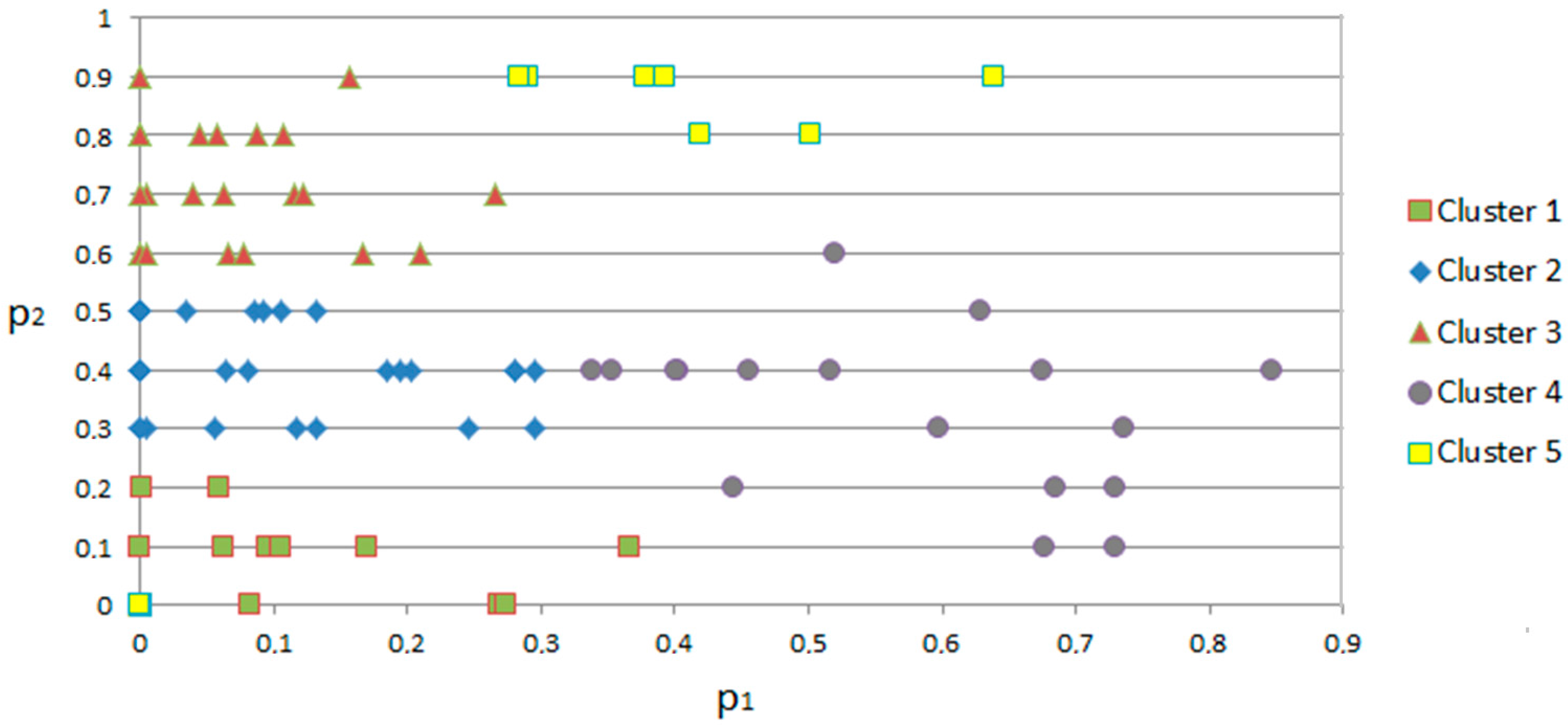
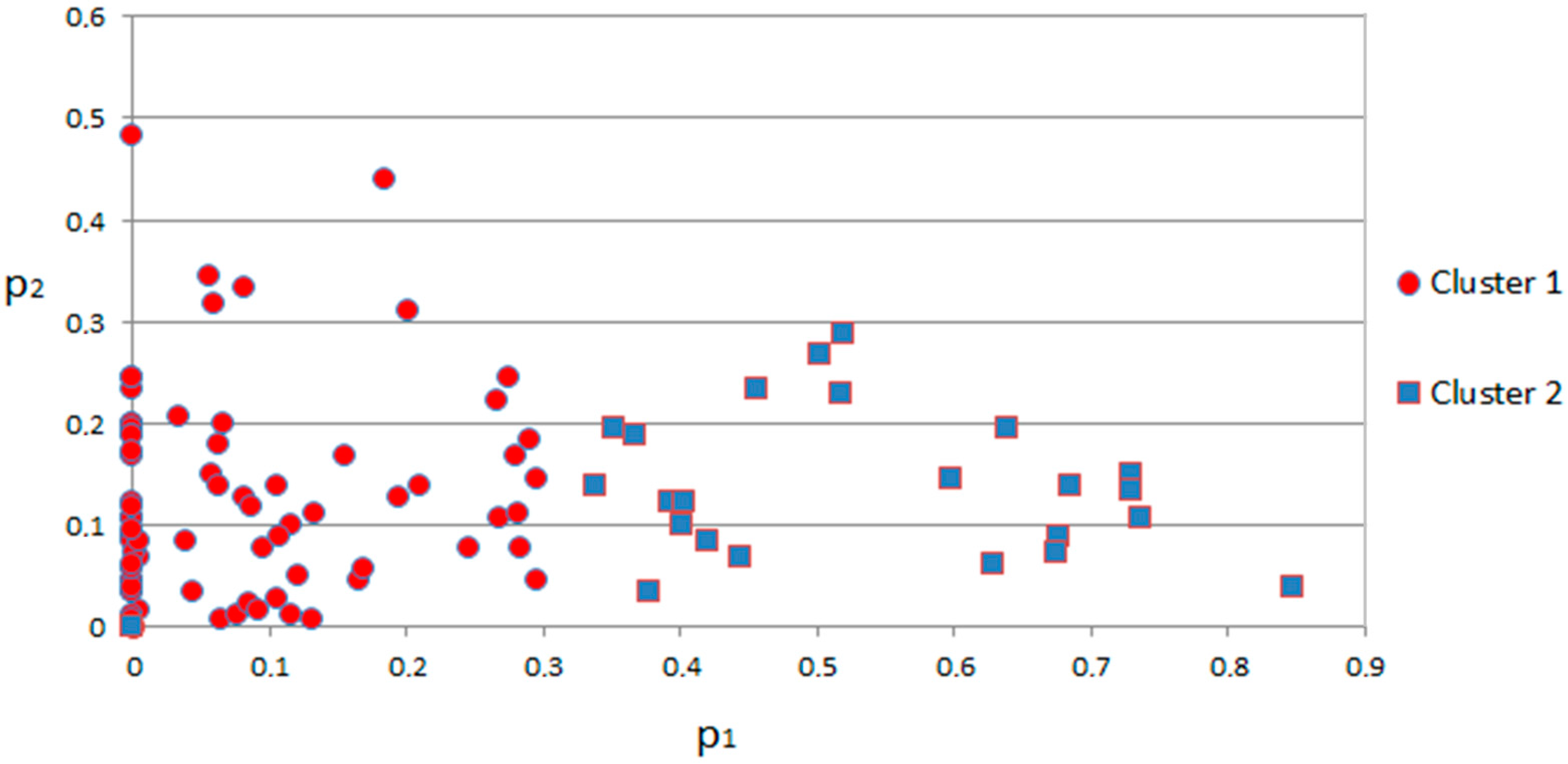
Keeping in mind that the smaller the classification parameters are the more reliable are considered the users, some interesting considerations about the quality of the classification can be drawn by analyzing the graph in
Figure 8 and the values of the coordinates in
Table 2.
The first cluster is the group containing the best users, namely those characterized by points that are closer to the origin. The second and third clusters, even though containing users with p1 coordinates as scattered as to those of the first cluster, show worst relative flexibility. The third cluster shows a cluster center with smaller p1 as compared to the first two clusters but all users show low relative flexibility and for this reason it is considered the worst cluster. The fourth and the fifth clusters are the worst, since users show worst (larger) p1 and p2 parameters as a whole.
This type of classification can be considered equally weighted on the basis of the two used parameters. This is due to the fact that the classification parameters show the same order of magnitude and a similar dispersion around a central value. Based on the two power target values, the algorithm chooses the users that will provide the flexibility service. In this case, out of 100, 67 customers will provide the flexibility service and out of these, the 17 users of the first cluster are called to take part to the program, while 35 users of the second cluster and 15 on a total of 24 users of the third, fourth and fifth clusters are discarded.
Using the flexibility provided by the cited users and aggregating their load request the following values of power are absorbed in the considered hour:
Average absorbed power in the considered hour, Pm_u = 900 W;
Average hourly power absorbed by the aggregate of the users, Ptot_u = 60.3 kW.
4.2.2. Results Analysis—Case 2
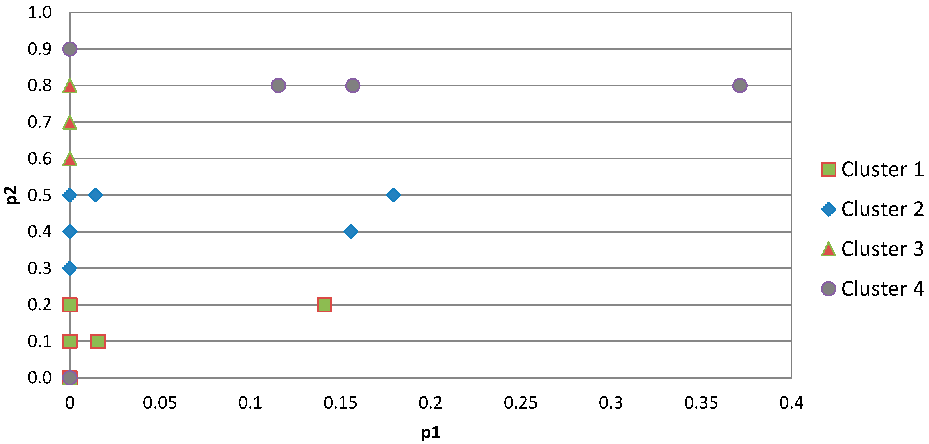
From the analysis of the graph in
Figure 9 and of the coordinates in
Table 3, some interesting considerations can be drawn. The first
cluster is the group of best users, namely those showing parameters that are closer to the origin. The second
cluster, even though showing p2 coordinates similar to the first is characterized by largely worse p1 values.
A classification of this type can be weighted on the basis of parameter p1 (namely |Pobb − (Pm + f)|). This is due to the fact that, even if the two parameters show the same order of magnitude, the one related to relative flexibility is more concentrated in a small range. A classification carried out following this logic can be considered optimal since it is correct to consider among equally reliable users those that have a flexibility promise that is closer to the target value Pobb.
On the basis of the two target values, also in this case, 67 users out of 100 provide the flexibility service, they all belong to the first cluster while the second cluster is discarded. Using the flexibility provided by the cited users and aggregating their load request the following values of power are absorbed in the considered hour:
average absorbed power in the considered hour, Pm_u = 900 W;
average hourly power absorbed by the aggregate of the users, Ptot_u = 60 kW
As it can be noted in both cases (1 and 2), the algorithm is able to cover the request formulated by the platform and fulfill the objectives.
4.3. Uniform and Controlled Power Absorption
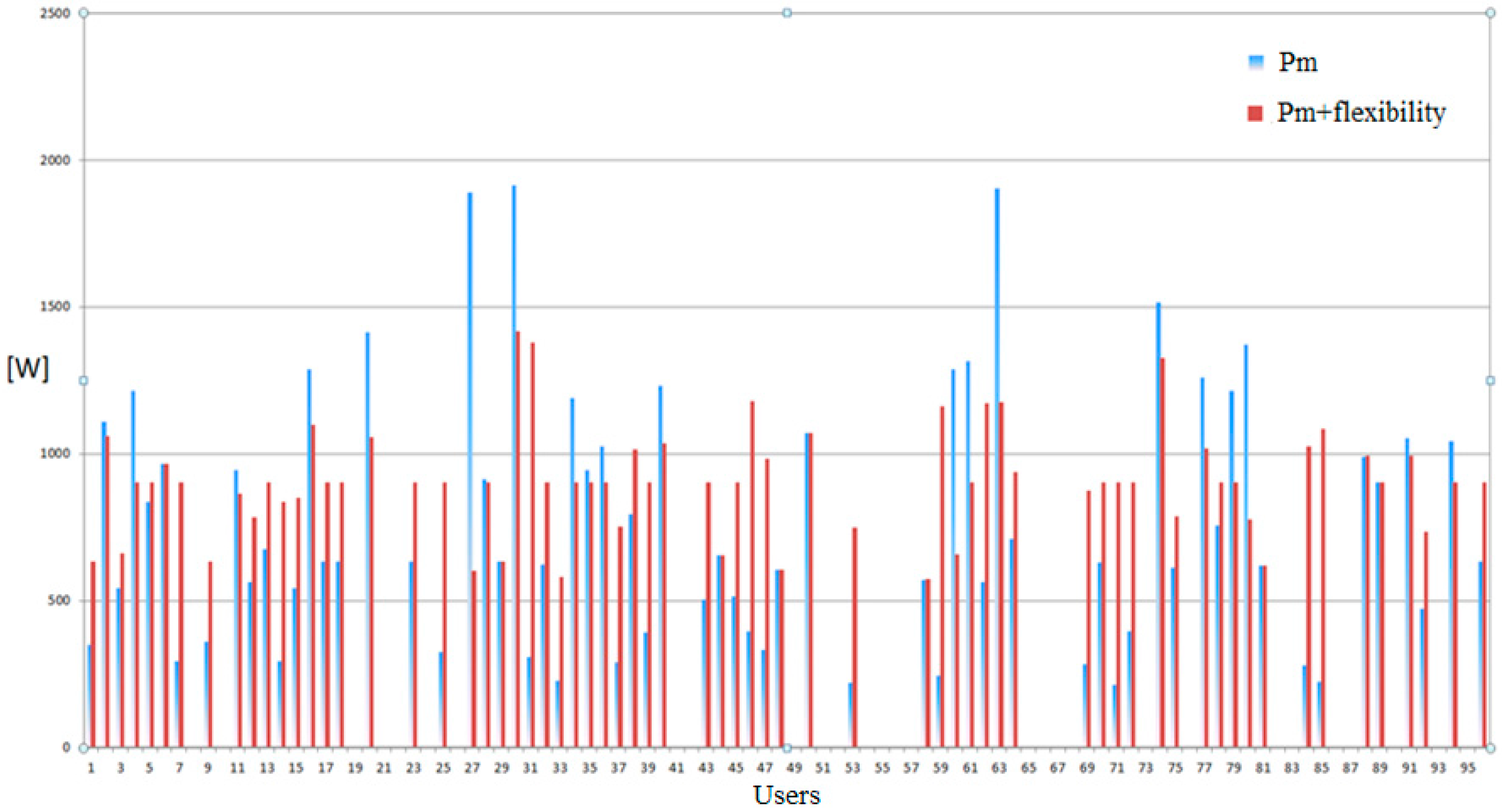
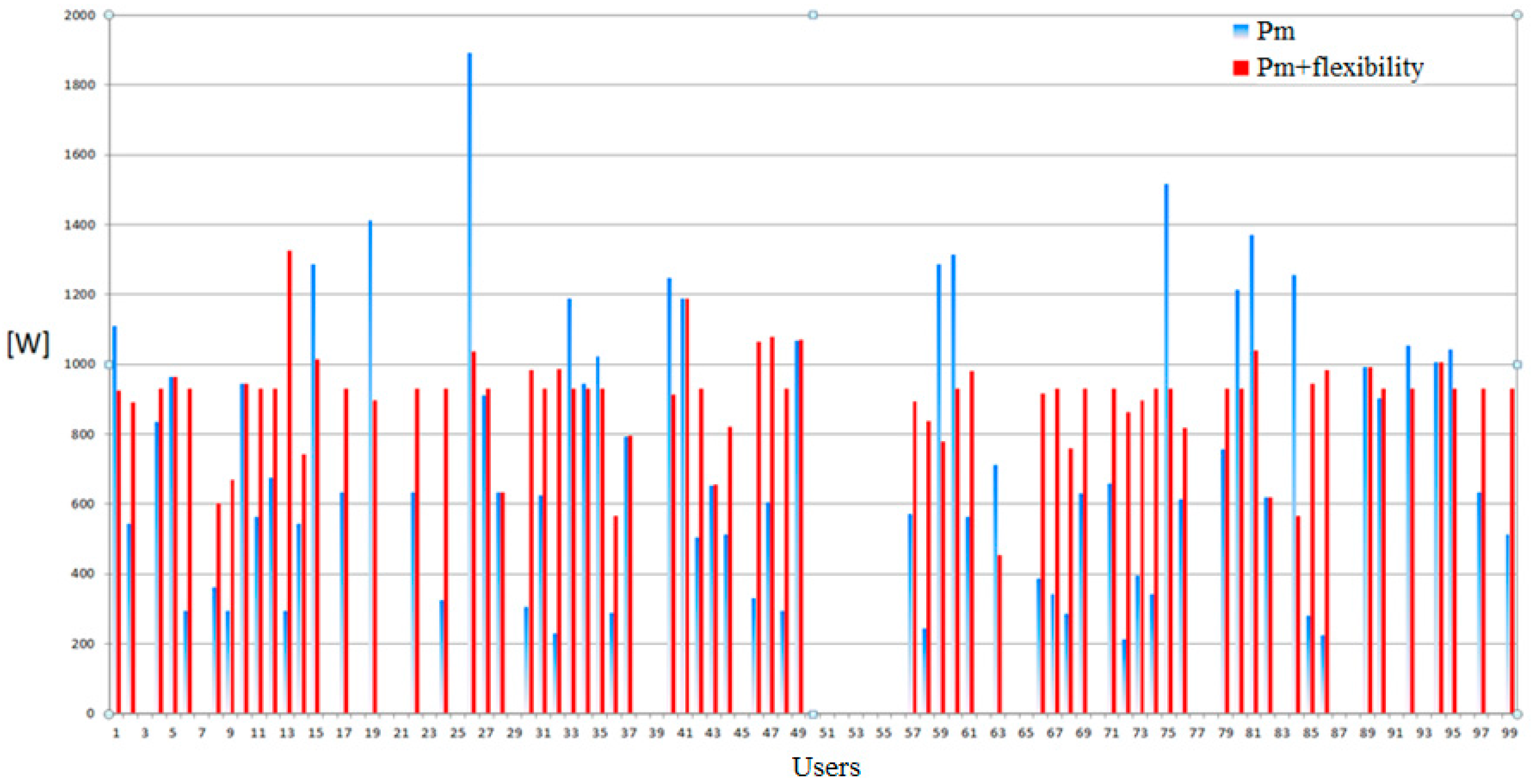
Figure 10 and
Figure 11 show a comparison between the average hourly power absorbed by the 100 users with and without flexibility in the two cases. It is evident that following the target values P
obb implies in both cases large benefits in terms of power absorbed by the users taking part to the service. The aggregated consumers indeed absorb an average hourly controllable power, in relation to the needs of the ancillary service market, and show a uniform behavior.
The above figures allow to identify which users among those that have subscribed in the platform (following the order of
Table 3), are called to take part to the flexibility service in this hour of the day.
4.4. Performance of the Algorithm
For better showing the performance of the clustering algorithm another application example its provided.
Table 4 and
Table 5 report two different communities of customers. In
Table 4 are listed 100 customers showing highly dispersed values of f_up and f_down. On the contrary,
Table 5 shows 100 customers with similar values of f_up and f_down.
Figure 12 and
Figure 13 show the users distribution on the plane p1-p2 for both the cases, demonstrating the good performance of the clustering algorithm also varying the values of f_up and f_down.
5. Conclusions
Some conclusions can be given. The paper has proposed a new framework for loads aggregation in the context of the liberalized energy market. Individual customers can join a load aggregation program through a software platform. Through the platform, the features of the users are evaluated and the customers are clustered according to their reliability and to the width of range of regulation allowed.
The proposed aggregation platform, the clustering method and the algorithm proposed in this work are designed for allowing the participation of the aggregated end-users to the ancillary service market. Nevertheless, the proposed system can be used also for power management.
Some simulations have been done, showing the deployment of an effective clustering and the possibility to meet the target power demand at a given hour, according to each customer’s availability. In particular two cases have been examined. With regards to the results of the simulations, some other considerations can be given.
The number of aggregated users depends not only on the total requested power Ptot, but also by the average hourly power Pobb; indeed, increasing or lowering this latter value, the number of aggregated users can increase or decrease. In particular, if the platform asks the users to increase their own average hourly consumption, a smaller number of aggregated users will be needed to cover Ptot, if the tendency is opposite the number will increase. To explain this concept, the logic on which the platform would act resembles a container with given water capacity (Ptot) that can be filled with water with a given number of glasses of equal dimension (Pobb). On these numbers, the number of glasses needed to fill the container depends.
Acting on the target value Pobb can be useful if only a few users are reliable and many are not; in these conditions, increasing the target value Pobb, means to determine a smaller number of users to take part to the flexibility service.
As an example, in the case 2, increasing the value of Pobb from 900 W to 1500 W a reduction of the number of users taking part to the service decreases from 67 to 40, obtaining the following values of power:
average absorbed power in the considered hour, Pm_u = 1500 W;
average hourly power absorbed by the aggregate of the users, Ptot_u = 60 kW
On the contrary, if a larger number of users must be involved, it will be enough to decrease the value of Pobb. Lowering such value from 900 W to 700 W the following results can be attained, with an increase of the number of involved customers from 67 to 89:
Average absorbed power in the considered hour, Pm_u = 700 W;
Average hourly power absorbed by the aggregate of the users, Ptot_u = 60.2 kW
As a result, acting on the target value Pobb the number of users changes too, attaining the required objectives. Finally, the present paper has not discussed the issue of defining guidelines and benefits for the participation of end-users in the ancillary service market. The simplest solution is to remunerate the end-user proportionally to the provided flexibility. Nevertheless, this latter is a very topical issue and is currently widely discussed in many research papers. In a future extension of this work, we will explore how the effect of policies for remunerating DR programs can affect the user flexibility.

 ,
, 


