Impact of the Complementarity between Variable Generation Resources and Load on the Flexibility of the Korean Power System


Abstract
:1. Introduction
2. Flexibility Index: Ramping Capability Shortage Expectation
Ramping Capability Shortage Expectation (RSE)
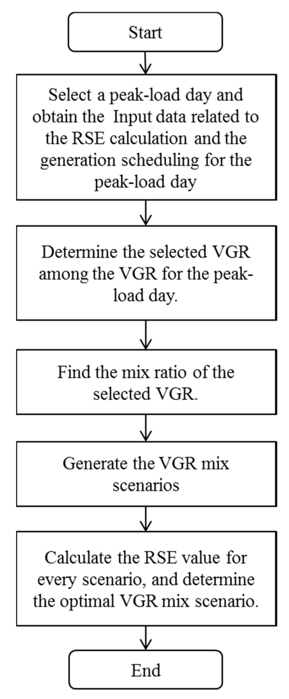
3. VGR Optimal Mix
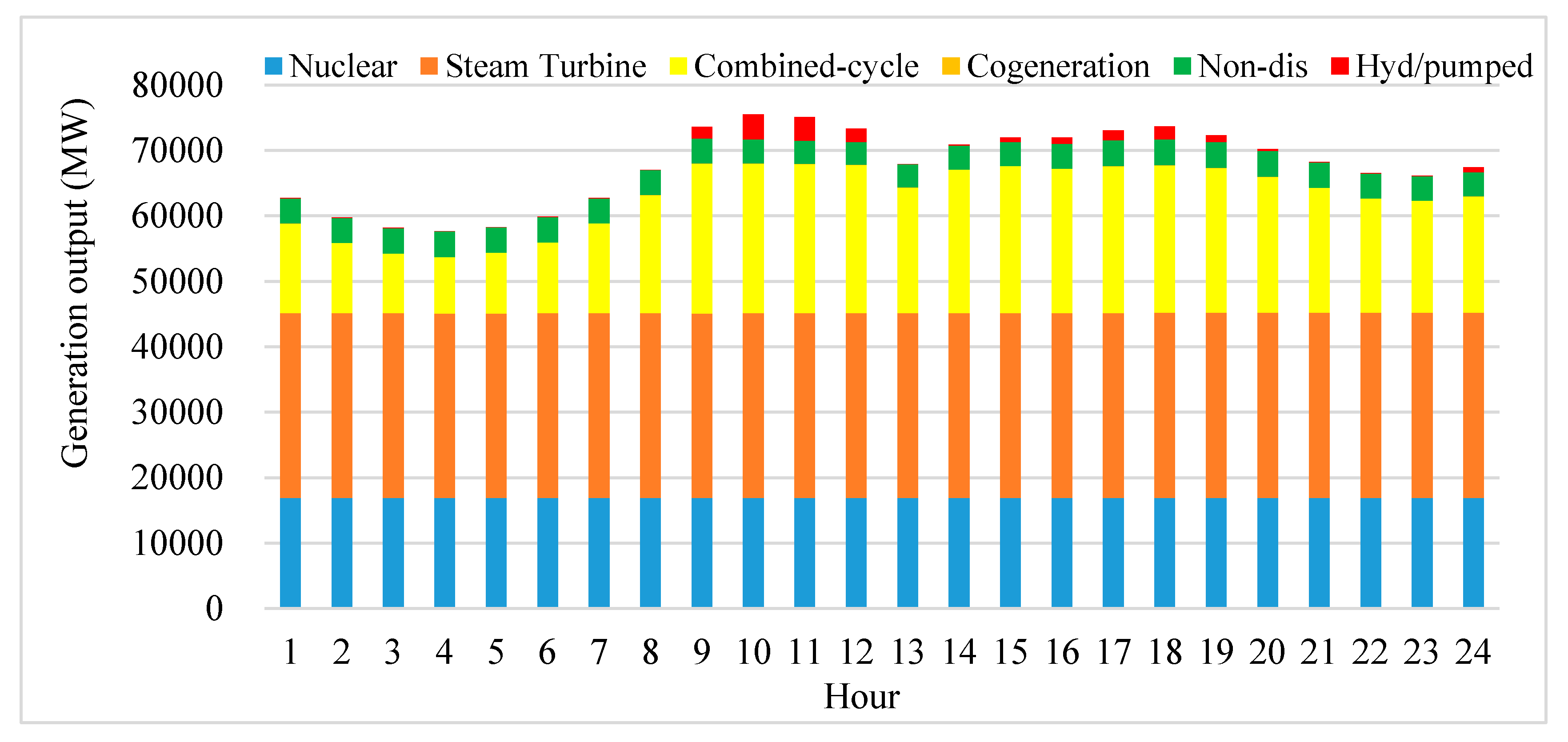
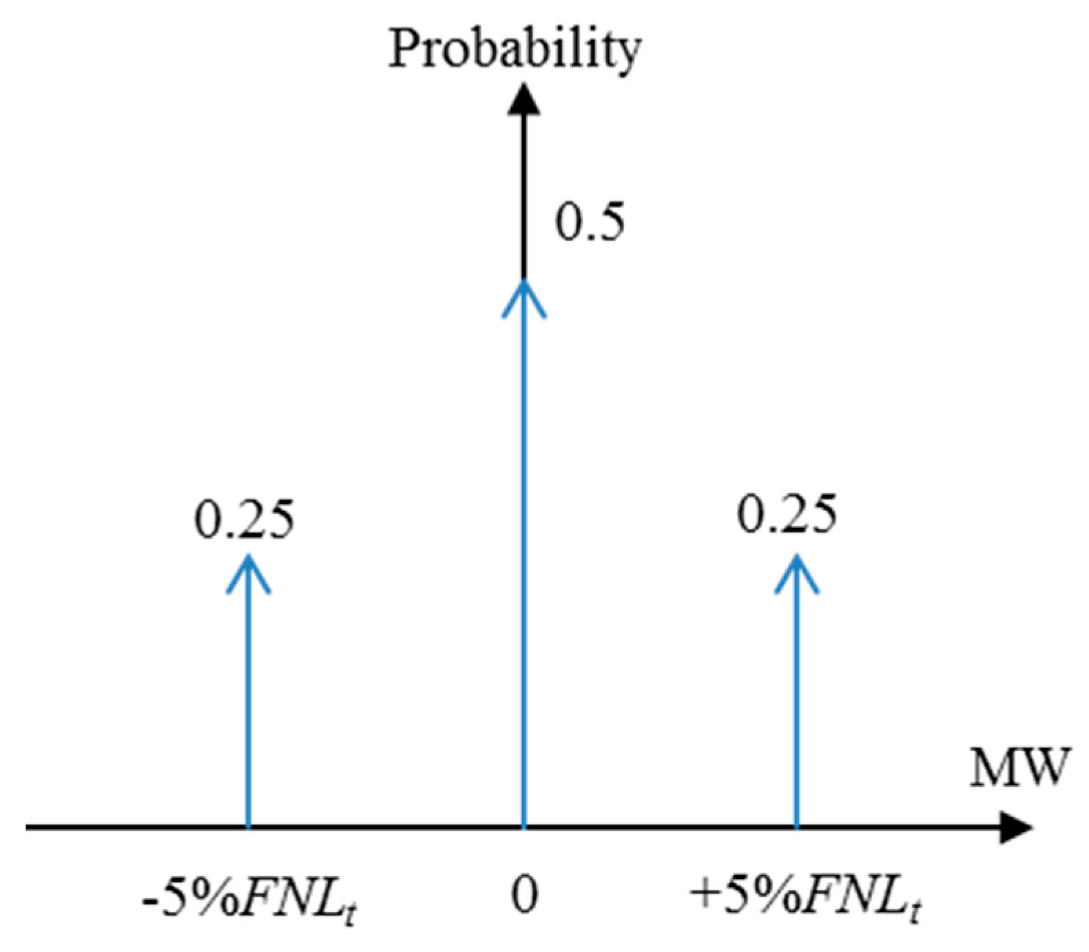
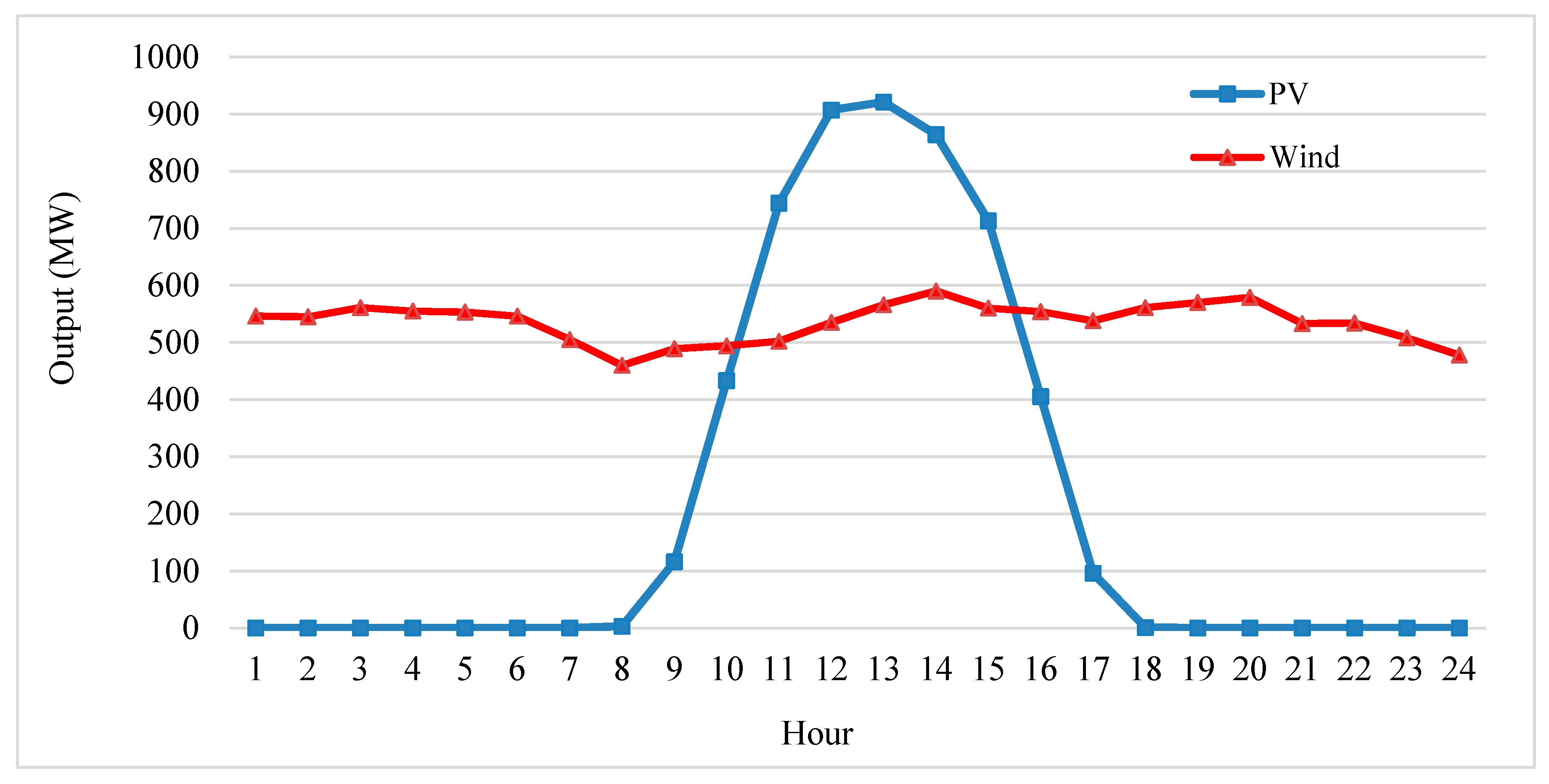
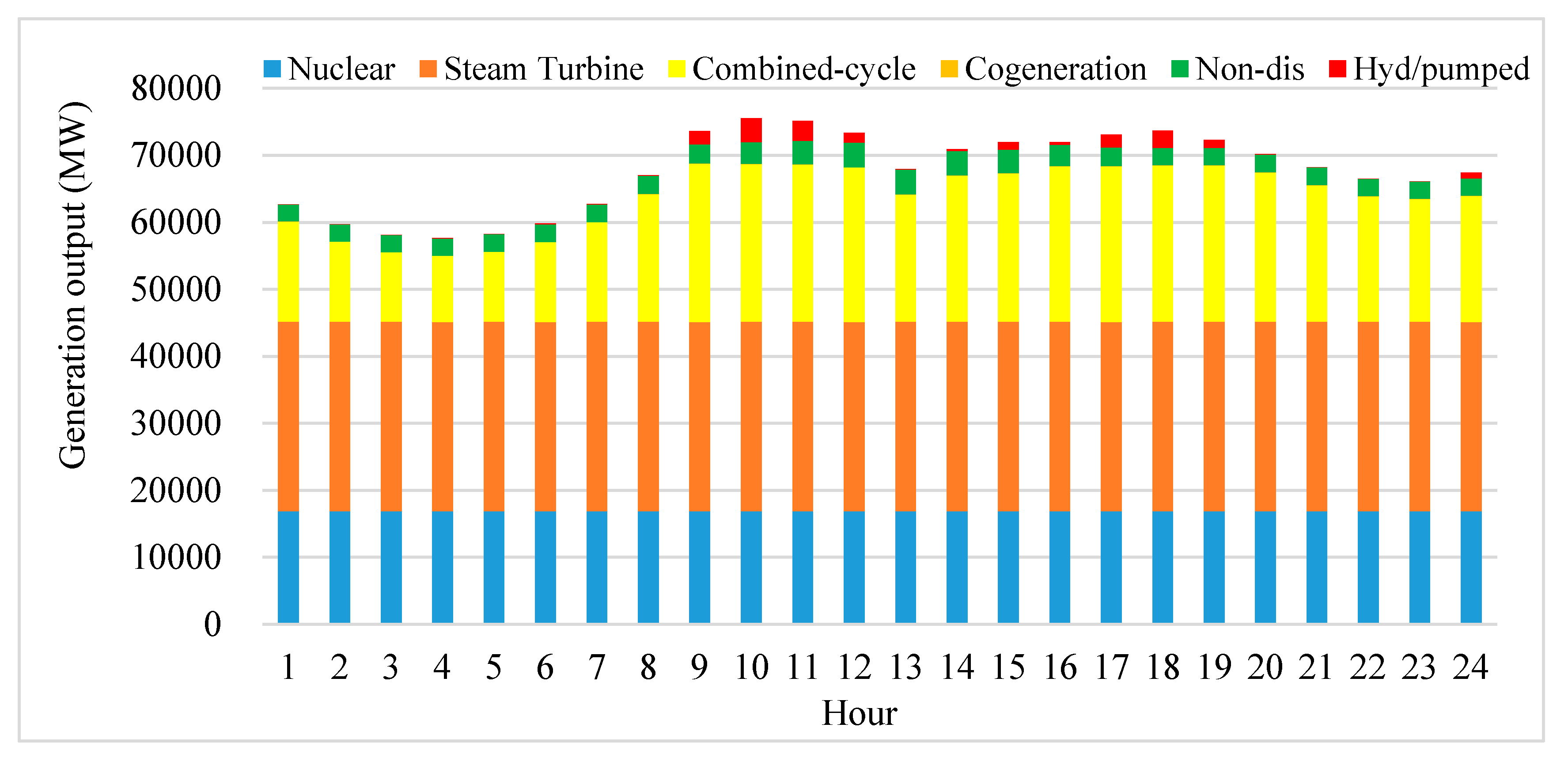
- Step 1. Select a peak-load day. The input data related to the RSE calculation and the generation scheduling for a day is required. For reference, the input data for the RSE calculation are as follows: load and VGR output profiles, generator’s failure and repair rates, forecast error distributions of the load and VGR output, and generation schedule result.
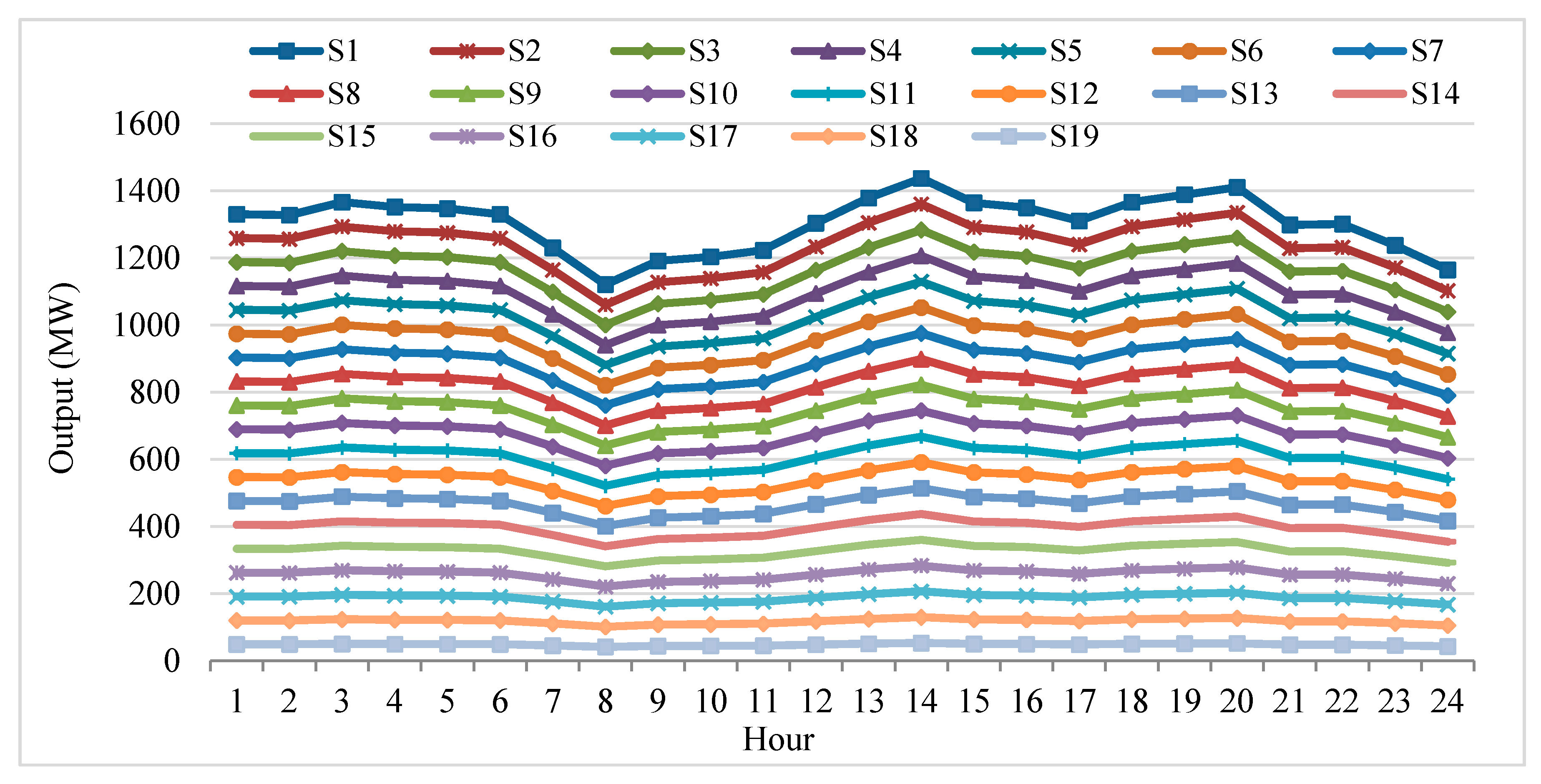
- Step 2. Select more than two VGRs from among the VGR for the day. For reference, all VGRs, of course, can be selected; however, selecting all VGRs may be inefficient because the share of some VGRs is too small to affect the flexibility.
- Step 3. Find the mix ratio of the selected VGR.
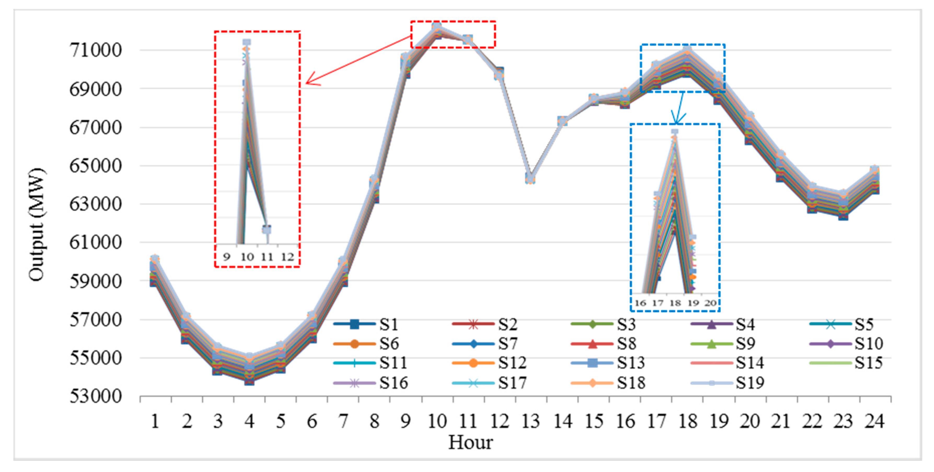
- Step 4. Generate the VGR mix scenarios, i.e., change the ratios in lexicographic order with a constant step size, keeping the same VGR penetration level:
- Step 5. Calculate the RSE value (i.e., flexibility) for every scenario, using Equations (5) and (6). The VGR mix scenario having the smallest RSE value is determined as the optimal VGR mix scenario.
4. Case Study
5. Conclusions
Acknowledgments
Author Contributions
Conflicts of Interest
Nomenclature
| Ai,t | Random variable representing availability of generator i at time t (1 if available, 0 otherwise) |
| αns | Ratio of non-selected VGR j to total VGR |
| αj | Ratio of selected VGR j to total VGR |
| c | Element of Ct−Δt |
| Ct−Δt | Set of combinations of Ai,t−Δt when Oi,t−Δt is nonzero for all i |
| e | Element of Et |
| Et | Set of NLFEt |
| FLt | Forecast load at time t |
| FNLt | Forecast net load at time t |
| FVGt | Forecast variable generation at time t |
| i | Index of generator |
| I | Set of generators |
| j | Index of VGR |
| LFEt | Random variable representing load forecast error at time t |
| NLFEt | Random variable representing net load forecast error at time t |
| Oi,t | Value representing whether generator i is online at time t or not |
| Pi,t | Output of generator i at time t |
| Pmax,i | Maximum output level of generator i |
| PHES | Pumped hydroelectric storage |
| Prob(·) | Probability in the brackets. |
| Probc[·] | Probability of c if condition [·] is satisfied, 0 otherwise. |
| RCRt | Ramping capability requirement at time t |
| rri | Ramp rate of generator i |
| RES | Renewable energy sources |
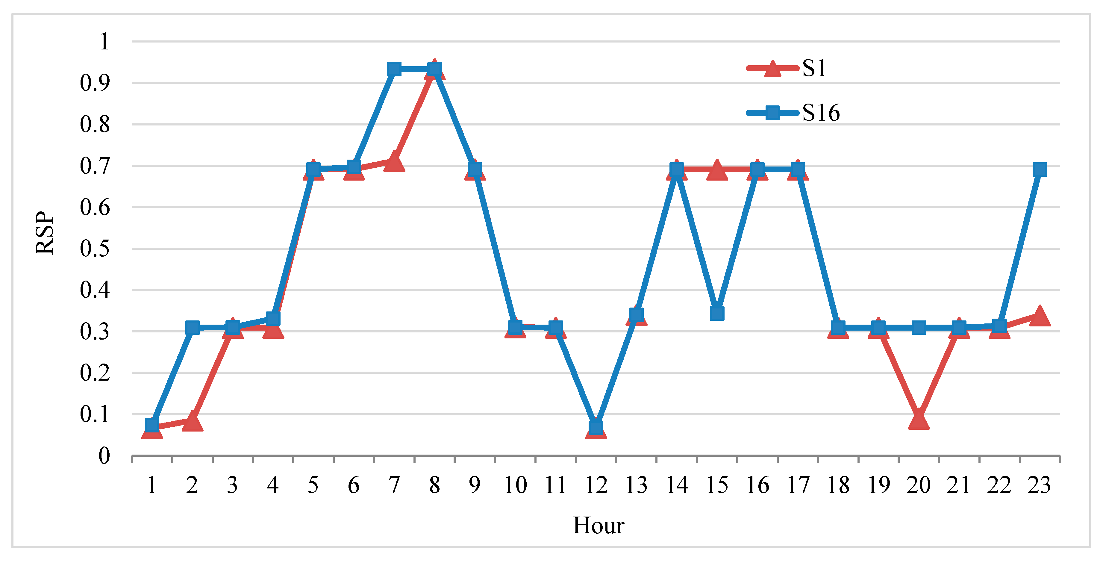
| RSPt | Ramping capability shortage probability at time t |
| SRCt | System ramping capability at time t |
| t | Index of time |
| Δt | Minimum interval between operating points |
| VG | Installed capacity of all VGR |
| VGj | Installed capacity of selected VGR j |
| VGns | Installed capacity of all nonselected VGRs |
| VGR | Variable generation resource |
| VGFEt | Random variable representing variable generation forecast error at time t |
References
- Graabak, I.; Korpås, M. Variability characteristics of european wind and solar power resources—A review. Energies 2016, 9, 449. [Google Scholar] [CrossRef]
- The Ministry of Trade, Industry and Energy. The 7th Basic Plan on Electricity Demand and Supply; MOTIE: Sejong-si, Korea, 2015.
- Min, C.-G.; Kim, M.-K. Net load carrying capability of generating units in power systems. Energies 2017, 10, 1221. [Google Scholar] [CrossRef]
- Min, C.-G.; Kim, M.-K. Flexibility-based reserve scheduling of pumped hydroelectric energy storage in Korea. Energies 2017, 10, 1478. [Google Scholar]
- Gabash, A.; Li, P. Active-reactive optimal power flow in distribution networks with embedded generation and battery storage. IEEE Trans. Power Syst. 2012, 27, 2026–2035. [Google Scholar] [CrossRef]
- Gabash, A.; Li, P. Flexible optimal operation of battery storage systems for energy supply networks. IEEE Trans. Power Syst. 2013, 28, 2788–2797. [Google Scholar] [CrossRef]
- Gabash, A.; Li, P. On variable reverse power flow-part i: Active-reactive optimal power flow with reactive power of wind stations. Energies 2016, 9, 121. [Google Scholar] [CrossRef]
- Gabash, A.; Li, P. On variable reverse power flow-part ii: An electricity market model considering wind station size and location. Energies 2016, 9, 235. [Google Scholar] [CrossRef]
- Díaz-González, F.; Hau, M.; Sumper, A.; Gomis-Bellmunt, O. Participation of wind power plants in system frequency control: Review of grid code requirements and control methods. Renew. Sustain. Energy Rev. 2014, 34, 551–564. [Google Scholar] [CrossRef]
- Widén, J.; Carpman, N.; Castellucci, V.; Lingfors, D.; Olauson, J.; Remouit, F.; Bergkvist, M.; Grabbe, M.; Waters, R. Variability assessment and forecasting of renewables: A review for solar, wind, wave and tidal resources. Renew. Sustain. Energy Rev. 2015, 44, 356–375. [Google Scholar] [CrossRef]
- Xiao, L.; Lin, L.; Liu, Y. Discussions on the architecture and operation mode of future power grids. Energies 2011, 4, 1025–1035. [Google Scholar] [CrossRef]
- Solomon, A.A.; Faiman, D.; Meron, G. Grid matching of large-scale wind energy conversion systems, alone and in tandem with large-scale photovoltaic systems: An Israeli case study. Energy Policy 2010, 38, 7070–7081. [Google Scholar] [CrossRef]
- Halamay, D.A.; Brekken, T.K.; Simmons, A.; McArthur, S. Reserve requirement impacts of large-scale integration of wind, solar, and ocean wave power generation. IEEE Trans. Sustain. Energy 2011, 2, 321–328. [Google Scholar] [CrossRef]
- Prasad, A.A.; Taylor, R.A.; Kay, M. Assessment of solar and wind resource synergy in Australia. Appl. Energy 2017, 190, 354–367. [Google Scholar] [CrossRef]
- Bett, P.E.; Thornton, H.E. The climatological relationships between wind and solar energy supply in Britain. Renew. Energy 2016, 87, 96–110. [Google Scholar] [CrossRef]
- Huang, Q.; Shi, Y.; Wang, Y.; Lu, L.; Cui, Y. Multi-turbine wind-solar hybrid system. Renew. Energy 2015, 76, 401–407. [Google Scholar] [CrossRef]
- Solomon, A.; Kammen, D.M.; Callaway, D. Investigating the impact of wind-solar complementarities on energy storage requirement and the corresponding supply reliability criteria. Appl. Energy 2016, 168, 130–145. [Google Scholar] [CrossRef]
- Hoicka, C.E.; Rowlands, I.H. Solar and wind resource complementarity: Advancing options for renewable electricity integration in Ontario, Canada. Renew. Energy 2011, 36, 97–107. [Google Scholar] [CrossRef]
- Huva, R.; Dargaville, R.; Caine, S. Prototype large-scale renewable energy system optimisation for Victoria, Australia. Energy 2012, 41, 326–334. [Google Scholar] [CrossRef]
- Jerez, S.; Trigo, R.; Sarsa, A.; Lorente-Plazas, R.; Pozo-Vázquez, D.; Montávez, J. Spatio-temporal complementarity between solar and wind power in the Iberian Peninsula. Energy Procedia 2013, 40, 48–57. [Google Scholar] [CrossRef]
- Patsialis, T.; Kougias, I.; Kazakis, N.; Theodossiou, N.; Droege, P. Supporting renewables’ penetration in remote areas through the transformation of non-powered dams. Energies 2016, 9, 1054. [Google Scholar] [CrossRef]
- Beluco, A.; de Souza, P.K.; Krenzinger, A. A dimensionless index evaluating the time complementarity between solar and hydraulic energies. Renew. Energy 2008, 33, 2157–2165. [Google Scholar] [CrossRef]
- Kougias, I.; Szabó, S.; Monforti-Ferrario, F.; Huld, T.; Bódis, K. A methodology for optimization of the complementarity between small-hydropower plants and solar pv systems. Renew. Energy 2016, 87, 1023–1030. [Google Scholar] [CrossRef]
- Fang, W.; Huang, Q.; Huang, S.; Yang, J.; Meng, E.; Li, Y. Optimal sizing of utility-scale photovoltaic power generation complementarily operating with hydropower: A case study of the world’s largest hydro-photovoltaic plant. Energy Convers. Manag. 2017, 136, 161–172. [Google Scholar] [CrossRef]
- Schmidt, J.; Cancella, R.; Pereira, A.O. An optimal mix of solar pv, wind and hydro power for a low-carbon electricity supply in Brazil. Renew. Energy 2016, 85, 137–147. [Google Scholar] [CrossRef]
- Beluco, A.; de Souza, P.K.; Krenzinger, A. A method to evaluate the effect of complementarity in time between hydro and solar energy on the performance of hybrid hydro pv generating plants. Renew. Energy 2012, 45, 24–30. [Google Scholar] [CrossRef]
- Francois, B.; Borga, M.; Creutin, J.-D.; Hingray, B.; Raynaud, D.; Sauterleute, J.-F. Complementarity between solar and hydro power: Sensitivity study to climate characteristics in northern-Italy. Renew. Energy 2016, 86, 543–553. [Google Scholar] [CrossRef]
- Min, C.-G.; Park, J.K.; Hur, D.; Kim, M.-K. A risk evaluation method for ramping capability shortage in power systems. Energy 2016, 113, 1316–1324. [Google Scholar] [CrossRef]
- Borges, C.L.T. An overview of reliability models and methods for distribution systems with renewable energy distributed generation. Renew. Sustain. Energy Rev. 2012, 16, 4008–4015. [Google Scholar] [CrossRef]
- Master’s Space. M-Core User’s Manual; MS: Anyang-si, Korea, 2016. [Google Scholar]
- Li, L. Matlab User Manual; Matlab: Natick, MA, USA, 2001. [Google Scholar]
- Korea Power Exchange. Electric Power Statistics Information System. Available online: http://epsis.kpx.or.kr/epsis/ekesStaticMain.do?cmd=001001&flag=&locale=EN (accessed on 8 September 2017).
- Allan, R.N. Reliability Evaluation of Power Systems; Springer Science & Business Media: Berlin, Germany, 2013. [Google Scholar]


| Scenario | PV Ratio [%] | Wind Ratio [%] |
|---|---|---|
| S1 | 1.3 | 93.4 |
| S2 | 6.3 | 88.4 |
| S3 | 11.3 | 83.4 |
| S4 | 16.3 | 78.4 |
| S5 | 21.3 | 73.4 |
| S6 | 26.3 | 68.4 |
| S7 | 31.3 | 63.4 |
| S8 | 36.3 | 58.4 |
| S9 | 41.3 | 53.4 |
| S10 | 46.3 | 48.4 |
| S11 | 51.3 | 43.4 |
| S12 | 56.3 | 38.4 |
| S13 | 61.3 | 33.4 |
| S14 | 66.3 | 28.4 |
| S15 | 71.3 | 23.4 |
| S16 | 76.3 | 18.4 |
| S17 | 81.3 | 13.4 |
| S18 | 86.3 | 8.4 |
| S19 | 91.3 | 3.4 |
| Scenario | RSE [hours/day] |
|---|---|
| S1 | 9.9435 |
| S2 | 10.6189 |
| S3 | 10.2710 |
| S4 | 10.6162 |
| S5 | 10.6172 |
| S6 | 10.5893 |
| S7 | 10.3990 |
| S8 | 10.6027 |
| S9 | 10.6156 |
| S10 | 10.6136 |
| S11 | 10.6273 |
| S12 | 10.6346 |
| S13 | 10.6370 |
| S14 | 10.6192 |
| S15 | 10.6417 |
| S16 | 10.6500 |
| S17 | 10.6106 |
| S18 | 10.5961 |
| S19 | 10.6263 |
© 2017 by the authors. Licensee MDPI, Basel, Switzerland. This article is an open access article distributed under the terms and conditions of the Creative Commons Attribution (CC BY) license (http://creativecommons.org/licenses/by/4.0/).
Share and Cite
Min, C.-G.; Kim, M.-K. Impact of the Complementarity between Variable Generation Resources and Load on the Flexibility of the Korean Power System. Energies 2017, 10, 1719. https://doi.org/10.3390/en10111719
Min C-G, Kim M-K. Impact of the Complementarity between Variable Generation Resources and Load on the Flexibility of the Korean Power System. Energies. 2017; 10(11):1719. https://doi.org/10.3390/en10111719
Chicago/Turabian StyleMin, Chang-Gi, and Mun-Kyeom Kim. 2017. "Impact of the Complementarity between Variable Generation Resources and Load on the Flexibility of the Korean Power System" Energies 10, no. 11: 1719. https://doi.org/10.3390/en10111719
APA StyleMin, C.-G., & Kim, M.-K. (2017). Impact of the Complementarity between Variable Generation Resources and Load on the Flexibility of the Korean Power System. Energies, 10(11), 1719. https://doi.org/10.3390/en10111719