Transactive-Market-Based Operation of Distributed Electrical Energy Storage with Grid Constraints

Abstract

In a transactive energy market, distributed energy resources (DERs) such as dispatchable distributed generators (DGs), electrical energy storages (EESs), distribution-scale load aggregators (LAs), and renewable energy sources (RESs) have to earn their share of supply or demand through a bidding process. In such a market, the distribution system operator (DSO) may optimally schedule these resources, first in a forward market, i.e., day-ahead, and in a real-time market later on, while maintaining a reliable and economic distribution grid. In this paper, an efficient day-ahead scheduling of these resources, in the presence of interaction with wholesale market at the locational marginal price (LMP), is studied. Due to inclusion of EES units with integer constraints, a detailed mixed integer linear programming (MILP) formulation that incorporates simplified DistFlow equations to account for grid constraints is proposed. Convex quadratic line and transformer apparent power flow constraints have been linearized using an outer approximation. The proposed model schedules DERs based on distribution locational marginal price (DLMP), which is obtained as the Lagrange multiplier of the real power balance constraint at each distribution bus while maintaining physical grid constraints such as line limits, transformer limits, and bus voltage magnitudes. Case studies are performed on a modified IEEE 13-bus system with high DER penetration. Simulation results show the validity and efficiency of the proposed model.

1. Introduction

Market-driven operation of the electric distribution system has recently gained considerable research momentum due to an increasing deployment of various distributed energy resources (DERs) such as renewable energy sources (RESs), electrical energy storages (EESs), dispatchable distributed generation (DG) units, and load aggregators (LAs) [1,2,3,4]. With value as the key operation parameter, transaction-based modeling of DERs in the distribution system operator’s (DSO’s) market is becoming increasingly popular [2]. The study of transactive markets for distribution systems have become particularly interesting due to the interdependency of the wholesale electricity market dispatch to the economic and feasible operation of DERs and the distribution grid.

The structure of the electricity grid plays an important role in the way transactive markets are designed. Typically seen hierarchically layered, the independent system operator (ISO) in the top layer, acting as the wholesale market auctioneer, would consider every DSO as a pricing node that operates locational marginal price (LMP) markets [1]. In the lower layer, the DSO may use forecasted or post-wholesale market dispatches and LMPs to implement a similar energy auction within its own territory, and properly perform in the wholesale market bidding. In the DSO’s market, due to stringent reliability metrics and differences in how various DERs physically function, these resources need to be distinctively handled and modeled for efficient and reliable operation.

Proper DER bidding models are necessary to perform efficient transactive energy markets. For example, loads must be aggregated carefully to include bidding for both traditional and price sensitive loads that are willing to participate in the market and provide demand response services. Load and resource aggregation has been proposed by many researchers as an effective way to meet user demand by bidding on their behalf in the electricity market [5,6,7,8]. Different aggregator models have been proposed that may be incentivized to aggregate classical fixed and price responsive loads, and bid into the distribution market [9,10,11].

Similarly, EES units are crucial resources that play a vital role in the operation, integration, and management of other DERs due to their energy storing capability. An EES unit can provide a wide range of grid services that are valuable in addressing operational reliability challenges resulting from large-scale integration of RESs, such as resource variability, temporal mismatch between generation and demand, forecast uncertainty, and stability impacts [12]. EES units have great potential to help form deeper penetrations of renewable energy into electricity grids and deliver efficient, low-cost, and fundamental grid services [13]. EES operation, however, is restricted by certain physical constraints depending on the unit’s type and technology [14]. Some EES technologies have different depths of discharge (batteries are typically not discharged completely and depth of discharge refers to the extent to which they are discharged), charging/discharging and self-discharging efficiencies. Frequent charging and discharging of EES causes degradation and decreases the unit’s lifetime. Therefore, proper modeling of these constraints is necessary in order to operate EES units in the transactive environment.

Dispatchable and non-dispatchable DGs are another type of distribution-level DER that can participate in the DSO’s market. Dispatchable DGs, ranging from a few hundred kilowatts to a few megawatts, need to be modeled differently than that of their ISO-level counterparts as they are small units that may not be subject to ramp rates or start-up and shut-down costs. Non-dispatchable DGs, such as RESs that are stochastic in nature, provide cheap and clean energy, and need to be wisely included in the DSO’s market model.

In addition to the aforementioned DER types, distribution grid constraints such as line limits, transformer limits, and bus voltages are key considerations in the design of the DSO’s market. A certain schedule of DERs may be profitable from an economic perspective but may violate grid constraints and cause reliability issues. Therefore, models considering both economics and grid constraints are necessary in order to efficiently utilize these resources.

There are few studies that introduce distinctive concepts and models for the DSO’s electricity market [1,15,16]. In [1,15], the transactive DSO market model has been conceptualized without detailed formulation. In [16], a distribution market operator has been introduced that administers optimal scheduling of DERs, which include DGs and loads, while interacting with the ISO. However, this model does not include EES units and grid constraints such as bus voltages.

In this paper, we propose a day-ahead transactive energy auction for a DSO with high penetration of DERs, including DGs, EES units, LAs, and RESs, while considering distribution grid constraints. By allowing power injections at wholesale LMP, the DSO runs a double auction based on bids from different types of DERs to maximize social surplus while accounting for line limits, transformer limits, bus voltages, and the DER’s constraints. Due to inclusion of EES units with integer constraints, a detailed mixed integer linear programming (MILP) formulation, that incorporates simplified DistFlow equations to account for grid constraints, is proposed. The convex quadratic line and transformer apparent power flow constraints are linearized using an outer approximation. The proposed model clears the market at distribution locational marginal price (DLMP) as the Lagrange multiplier of the real power balance constraint at each distribution bus.

The rest of this paper is organized as follows: Section 2 provides the mathematical formulation. Section 3 presents the results, and Section 4 concludes the paper. Nomenclature is provided in the Abbreviations and Nomenclature.

2. Mathematical Formulation

In the proposed model, when the DSO receives the LMP from the ISO, it asks for bids from DG units, EES units, and LAs for each timeslot of the scheduling horizon. The LAs are assumed capable of aggregating their customers demand and dividing them into blocks of bids for each timeslot. A block of bid includes the monetary bid and the maximum amount of energy a LA is willing to purchase at that bid. Since all customers served by a LA are not price responsive, the first block of the LA’s bid is considered a mere energy amount with no monetary bid, representing the base load demand forecast of the LA that needs to be served at market clearing price (MCP) under any circumstance [17]. The rest of the LA’s bid blocks need to contain both monetary and energy amounts representing the aggregation of price responsive loads for participation in the energy auction.

DG units are considered to submit a three to four block bid representing the price and maximum amount they want to supply at each block. The DGs in this paper are assumed small units of fast ramping capability with no start-up or shut-down costs. Thus, the ramping rate constraints and start-up/shut-down costs of these units are not necessary to be included in the model. When required, these constraints can be easily incorporated [18].

Due to their non-dispatchable nature, it is assumed in this paper that RESs only provide their hourly forecast to the DSO to be cleared at MCP, without placing any monetary bid to avoid possible curtailment because of overbidding. Interested readers are referred to [19,20,21] for other bidding strategies of RESs in the electricity market.

The EES units are considered to bid their charging and discharging costs and provide their physical unit constraints parameters to the DSO. The EES constraints parameters include minimum/maximum state of charge (SOC), minimum/maximum power rate, minimum number of consecutive charging/discharging hours, and the initial SOC.

Upon reception of the DER bids and LMP information, the DSO runs its energy auction to allocate energy for least cost operation and clears the market at MCP, i.e., DLMP. An illustration of the MCP as the intersection of the traditional aggregate supply-demand curves is shown in Figure 1. Note that the LA does not place any monetary bid in its first block; therefore, the aggregate demand curve is shifted by an amount equal to the base load, i.e., r1. While accounting for grid constraints, the DLMPs are obtained as the Lagrange multipliers of the supply-demand balance constraint at each distribution bus in the DSO’s scheduling problem for social surplus maximization. Pricing based on DLMP is extensively used in literature for distribution system congestion management, market clearing, and loss minimization [22,23,24,25], as it shows the true marginal cost of supplying the next increment of load.

Figure 2 shows a schematic of a modified IEEE 13-bus distribution system with DERs across different buses and the wholesale market injection modeled as DG1 at Bus 1. In other words, the net demand of the distribution system is modeled as the injection of DG1. The wholesale market LMP at the DSO bus is typically correlated with the demand drawn by the distribution system [26,27]. In [26], this correlation is approximated using a linear equation between LMP and the total demand drawn by the distribution system. Historical LMP and demand data are used to approximate the slope, i.e., elasticity of LMP. For an elastic LMP, the cost of supply from DG1 can be formulated as a quadratic function in the DSO’s auction, which in turn can be approximated using piecewise bid blocks similar to what is currently implemented in the wholesale electricity market for generation companies. Therefore, we assume that the LMP at the DSO bus is inelastic to the demand of the distribution system and can be represented as a single bid block composed of LMP and a high injection amount. Further blocks can simply be added to DG1’s bid to account for LMP elasticity. Note that with higher penetration of DERs that supply energy back to the grid, the wholesale market role can be similarly modeled as a bid block composed of LMP and a high demand amount, in which case the DSO may act as a supplier in the wholesale market. In our previous work, we model the interaction between the LMP and demand as a bilevel optimization problem [28]. In this research, we focus on modeling the transactive operation of the distribution system in day-ahead market and such interactions between LMP and demand is out of the scope of this paper.

We index DERs based on bus indices and each bus $i\in ℬ$ may be connected to different types of DERs, i.e., EES units, DGs, RESs, and LAs. The social surplus maximization of the system can be formulated as in Equation (1) subject to the system constraints given in Equations (2)–(35):

Minimize $\mathcal{C}$:

$$\mathcal{C}={\displaystyle \sum }_{i\in \mathcal{G}, t\in \mathcal{T},q\in \mathcal{Q}}{\mathrm{c}}_{i,q,t}^{\mathrm{G}}·p_{i,q,t}^{\mathrm{G}}+{\displaystyle \sum }_{i\in ℰ, t\in \mathcal{T}}{\hat{\mathrm{c}}}_{i,t}^{\mathrm{E}}·{\widehat{p}}_{i,t}^{\mathrm{E}}-{\displaystyle \sum }_{i\in ℰ, t\in \mathcal{T}}{\check{\mathrm{c}}}_{i,t}^{\mathrm{E}}·{\check{p}}_{i,t}^{\mathrm{E}}-{\displaystyle \sum }_{i\in \mathcal{A}, t\in \mathcal{T},r\in \left\{ℛ\backslash 1\right\}}{\mathrm{c}}_{i,r,t}^{\mathrm{D}}·p_{i,r,t}^{\mathrm{D}}$$

(1)

Subject to power flow, load and DG units, line flow, and EES unit constraints

The objective function in Equation (1) minimizes the operational cost of the system by scheduling least cost generation, least cost energy extraction, and high value energy injections and loads while meeting the DER’s and grid’s constraints. The fourth term in the right hand side of Equation (1) is modeled for $r>1$ to account only for load blocks that bid in the DSO market. The constraints in Equation (1) are explained and formulated next.

(1) Power flow constraints:

In this study, simplified DistFlow equations that have been extensively used in the literature [29,30,31,32,33] have been adopted to set up the distribution system grid constraints. For a radial distribution feeder, as shown in Figure 3, simplified DistFlow equations for every line segment $ij\in ℒ$ can be written as in Equations (2)–(4) for all time $t\in \mathcal{T}$:

$$P_{ij,t}={{\displaystyle \sum }}_k{P}_{jk,t}+p_{j,t}$$

(2)

$$Q_{ij,t}={{\displaystyle \sum }}_k{Q}_{jk,t}+q_{j,t}$$

(3)

$$v_{j,t}=v_{i,t}-\left({\mathrm{r}}_{ij}{P}_{ij,t}+{\mathrm{x}}_{ij}{Q}_{ij,t}\right){\mathrm{V}}_{1,t}{}^{-1}$$

(4)

Here, $v_{j,t}$ is node $j$’s per unit voltage at time $t$, $\left({\mathrm{r}}_{ij},{\mathrm{x}}_{ij}\right)$ is the line resistance/reactance and $\left(P_{ij,t},Q_{ij,t}\right)$ is the line real/reactive power flow at time $t$ for the line connecting bus $i$ to $j$. At time t, the net real and reactive power injection into each bus $j\in ℬ$ is denoted by $\left(p_{j,t},q_{j,t}\right)$, and is given by Equations (5) and (6) as the difference of the LA’s demand, and the DG’s, RES’s, and EES unit’s generation:

$$p_{i,t}=p_{i,t}^{\mathrm{D}}-p_{i,t}^{\mathrm{G}}-p_{i,t}^{\mathrm{FR}}-p_{i,t}^{\mathrm{E}}$$

(5)

$$q_{i,t}=q_{i,t}^{\mathrm{D}}-q_{i,t}^{\mathrm{G}}-q_{i,t}^{\mathrm{FR}}-q_{i,t}^{\mathrm{E}}$$

(6)

The total systems real and reactive power balance constraint is given in Equation (7):

$$\left\{{{\displaystyle \sum }}_{i\in ℬ}{p}_{i,t}=0, {{\displaystyle \sum }}_{i\in ℬ}{q}_{i,t}=0\right\}$$

(7)

For every bus $j\in ℬ$, its per unit voltage has to lie within the normal operation range given by Equation (8):

$$0.95\le v_{j,t}\le 1.05$$

(8)

(2) LA and DG unit constraints:

In Equations (5) and (6), $p_{i,t}^{\mathrm{D}}$, $p_{i,t}^{\mathrm{G}}$, $q_{i,t}^{\mathrm{D}}$, and $q_{i,t}^{\mathrm{G}}$ are given and constrained by Equations (9)–(16):

$$p_{i,t}^{\mathrm{D}}={{\displaystyle \sum }}_r{p}_{i,r,t}^{\mathrm{D}}$$

(9)

$$0\le p_{i,r,t}^{\mathrm{D}}\le {\overline{\mathrm{P}}}_{i,r}^{\mathrm{D}}$$

(10)

$${\underset{¯}{\mathrm{P}}}_i^{\mathrm{D}}\le p_{i,t}^{\mathrm{D}}\le {\overline{\mathrm{P}}}_i^{\mathrm{D}}$$

(11)

$$q_{i,t}^{\mathrm{D}}={\mathsf{\delta }}_i^{\mathrm{D}}·p_{i,t}^{\mathrm{D}}$$

(12)

$$p_{i,t}^{\mathrm{G}}={{\displaystyle \sum }}_q{p}_{i,q,t}^{\mathrm{G}}$$

(13)

$$0\le p_{i,q,t}^{\mathrm{G}}\le {\overline{\mathrm{P}}}_{i,q}^{\mathrm{G}}$$

(14)

$${\underset{¯}{\mathrm{P}}}_i^{\mathrm{G}}\le p_{i,t}^{\mathrm{G}}\le {\overline{\mathrm{P}}}_i^{\mathrm{G}}$$

(15)

$$-{\mathsf{\delta }}_i^{\mathrm{G}}·p_{i,t}^{\mathrm{G}}\le q_{i,t}^{\mathrm{G}}\le {\mathsf{\delta }}_i^{\mathrm{G}}·p_{i,t}^{\mathrm{G}}$$

(16)

Constraints in Equations (9) and (13) ensure the sum of the allocated load and generation at each block must equal the total allocated load and generation at each timeslot, respectively. The block allocation, as well as their sums, have to stay within the given limits in Equations (10), (14) and (11), (15). Equations (12) and (16) show reactive power demand and generation of load and DG units, respectively. It is assumed that the reactive power demand of the load and the reactive generation capability of the DG units are also provided to the DSO as part of their bidding information. The reactive power generation of a generator is constrained by its reactive power capability curve. While only real power is priced, the involuntary production of reactive power incurs an opportunity cost for a generator [34,35]. In this paper, we assume that the reactive power provision capability of the generators lie within a certain percentage,$\mathsf{\delta }$, of their real power output. Furthermore, we do not price reactive power as it does not carry energy and does not directly contribute to fuel costs [36]. We note, however, that the reactive power can also be easily priced using the Lagrange multipliers of the reactive power balance constraint at each distribution bus.

(3) Line flow constraints:

Since each line segment, or transformer, has an apparent power flow (MVA) limit, the following convex quadratic constraint needs to be satisfied for all lines and transformers:

$$P_{ij,t}{}^2+Q_{ij,t}{}^2={\overline{\mathrm{S}}}_{ij}{}^2$$

An outer approximation of the above convex quadratic constraint has been leveraged to linearize the line flow constraints in order to use in the proposed MILP model. This approximation is given by Equation (17) for all $ij\in ℒ$ [37]:

$$\left|P_{ij,t}\right|+\left|Q_{ij,t}\right|\le \sqrt{2} {\overline{\mathrm{S}}}_{ij}$$

(17)

This constraint can simply be expanded into linear constraints for bidirectional power flow.

(4) EES unit constraints:

The EES unit’s SOC is given by Equation (18) for all $i\in ℰ$:

$$c_{i,t}^{\mathrm{E}}={\mathsf{\alpha }}_{i,t}{c}_{i,t-1}^{\mathrm{E}}-\Delta t\left({\hat{\mathsf{\alpha }}}_{i,t}{\widehat{p}}_{i,t-1}^{\mathrm{E}}-\frac{{\check{p}}_{i,t-1}^{\mathrm{E}}}{{\check{\mathsf{\alpha }}}_{i,t}}\right)$$

(18)

An EES unit’s energy is dissipated due to self-discharge (“leakage”), or during charging and discharging. These effects are respectively accounted for using the scaling coefficients,${\mathsf{\alpha }}_{i,t}$, ${\check{\mathsf{\alpha }}}_{i,t}$, and ${\hat{\mathsf{\alpha }}}_{i,t}$, each of which lies in the interval (0,1]. The EES unit’s SOC has to stay within a minimum and maximum SOC given by ${\underset{¯}{\mathrm{C}}}_i$ and ${\overline{\mathrm{C}}}_i$. The difference in grid power injection ${\check{p}}_{i,t}^{\mathrm{E}}$ and extraction ${\widehat{p}}_{i,t}^{\mathrm{E}}$ is modeled as the net grid injection $p_{i,t}^{\mathrm{E}}$ into the EES unit. Both ${\check{p}}_{i,t}^{\mathrm{E}}$ and ${\widehat{p}}_{i,t}^{\mathrm{E}}$ are bound by the EES charging/discharging power rates when the unit is scheduled. These constraints are respectively modeled in Equations (19)–(22). Note that in Equations (21) and (22), the EES unit is prohibited from charging and discharging at the same time by the two binary variables ${\check{𝓏}}_{i,t}$ and ${\widehat{𝓏}}_{i,t}$ and an additional binary constraint explained next:

$${\underset{¯}{\mathrm{C}}}_i\le c_{i,t}^{\mathrm{E}}\le {\overline{\mathrm{C}}}_i$$

(19)

$$p_{i,t}^{\mathrm{E}}={\check{p}}_{i,t}^{\mathrm{E}}-{\widehat{p}}_{i,t}^{\mathrm{E}}$$

(20)

$${\underset{¯}{\mathrm{E}}}_i{\check{𝓏}}_{i,t}\le {\check{p}}_{i,t}^{\mathrm{E}}\le {\overline{\mathrm{E}}}_i{\check{𝓏}}_{i,t}$$

(21)

$${\underset{¯}{\mathrm{E}}}_i{\widehat{𝓏}}_{i,t}\le {\widehat{p}}_{i,t}^{\mathrm{E}}\le {\overline{\mathrm{E}}}_i{\widehat{𝓏}}_{i,t}$$

(22)

Frequent charging and discharging of the EES unit decreases its lifetime [38,39,40]. In this paper, we restrict high number of charging/discharging cycles by including minimum charging/discharging hours using additional mixed integer constraints defined in Equations (23)–(35):

$$0\le {\widehat{𝓏𝒸}}_{i,t}\le \mathsf{{\rm T}}{\widehat{𝓏}}_{i,t}$$

(23)

$$\left(\mathsf{{\rm T}}+1\right){\widehat{𝓏}}_{i,t}-\mathsf{{\rm T}}\le {\widehat{𝓏𝒸}}_{i,t}-{\widehat{𝓏𝒸}}_{i,t-1}\le 1$$

(24)

$${\widehat{𝓏𝒸}}_{i,t}\ge {\widehat{ℳ}}_i{\widehat{𝓏n}}_{i,t+1}$$

(25)

$${\widehat{𝓏}}_{i,t}- {\widehat{𝓏}}_{i,t-1}={\widehat{𝓏m}}_{i,t}-{\widehat{𝓏n}}_{i,t}$$

(26)

$$0\le {\check{𝓏𝒸}}_{i,t}\le \mathsf{{\rm T}}{\check{𝓏}}_{i,t}$$

(27)

$$\left(\mathsf{{\rm T}}+1\right){\check{𝓏}}_{i,t}-\mathsf{{\rm T}}\le {\check{𝓏𝒸}}_{i,t}-{\check{𝓏𝒸}}_{i,t-1}\le 1$$

(28)

$${\check{𝓏𝒸}}_{i,t}\ge {\check{ℳ}}_i{\check{𝓏n}}_{i,t+1}$$

(29)

$${\check{𝓏}}_{i,t}-{\check{𝓏}}_{i,t-1}={\check{𝓏m}}_{i,t}-{\check{𝓏n}}_{i,t}$$

(30)

$${\check{𝓏}}_{i,t}+{\widehat{𝓏}}_{i,t}\le 1$$

(31)

$${\widehat{𝓏m}}_{i,t}+{\widehat{𝓏n}}_{i,t}\le 1$$

(32)

$${\check{𝓏m}}_{i,t}+{\check{𝓏n}}_{i,t}\le 1$$

(33)

$${\widehat{𝓏m}}_{i,t}+{\check{𝓏m}}_{i,t}\le 1$$

(34)

$${\widehat{𝓏n}}_{i,t}+{\check{𝓏n}}_{i,t}\le 1$$

(35)

Equation (23) guarantees that the discharging counter, ${\widehat{𝓏𝒸}}_{i,t}$, is nonnegative and does not exceed the scheduling horizon limit. Equation (24) adds to the discharging counter by one if the unit is discharging. Equation (25) constrains the discharging counter to be higher than the minimum number of consecutive discharging hours,${\widehat{ℳ}}_i$, of the EES unit by use of a not discharging indicator,${\widehat{𝓏n}}_{i,t}$. The not discharging indicator indicates a unity ‘1’ only when the unit stops discharging at which this constraint makes sure the counter is already higher than the specified minimum number of consecutive discharging hours. Equation (26) ensures discharging indicator, ${\widehat{𝓏m}}_{i,t}$, and not discharging indicator, ${\widehat{𝓏n}}_{i,t}$, are activated only when the discharging state, ${\widehat{𝓏}}_{i,t}$, is switched from unity ‘1’, to zero ‘0’ or vice versa. A similar explanation to that of Equations (23)–(26) holds in Equations (27)–(30) for the case of charging counter, ${\check{𝓏𝒸}}_{i,t}$, minimum number of consecutive charging hours,${\check{ℳ}}_i$, charging state, ${\check{𝓏}}_{i,t}$, and charging and not charging indicators, ${\check{𝓏m}}_{i,t}$ and ${\check{𝓏n}}_{i,t}$. Equation (31) ensures the EES unit does not charge and discharge at the same time. Equations (32)–(35) are additional constraints to ensure charging/discharging and not charging/not discharging indicators are not unity ‘1’ at the same time. By modeling and limiting the charging/discharging cycles of EES units in this way, the DSO can properly schedule these units for efficient operation while preventing its degradation due to increased charge/discharge frequency.

3. Simulation Results

Simulation results corroborate the theory presented in Section 2. GAMS/CPLEX [41] was used to implement the proposed MILP formulation on a modified IEEE 13-bus system with high penetration of DERs as depicted in Figure 2. Due to increased penetration of DERs, the overall load of the system was increased by 30%, while maintaining the same capacity in the substation transformer between lines 1 and 2. Two DGs were allocated in Buses 7 and 13. Four RESs (two wind, two solar) were positioned in Buses 4, 5, 9, and 13. Two EES units were allocated in Buses 3 and 7.

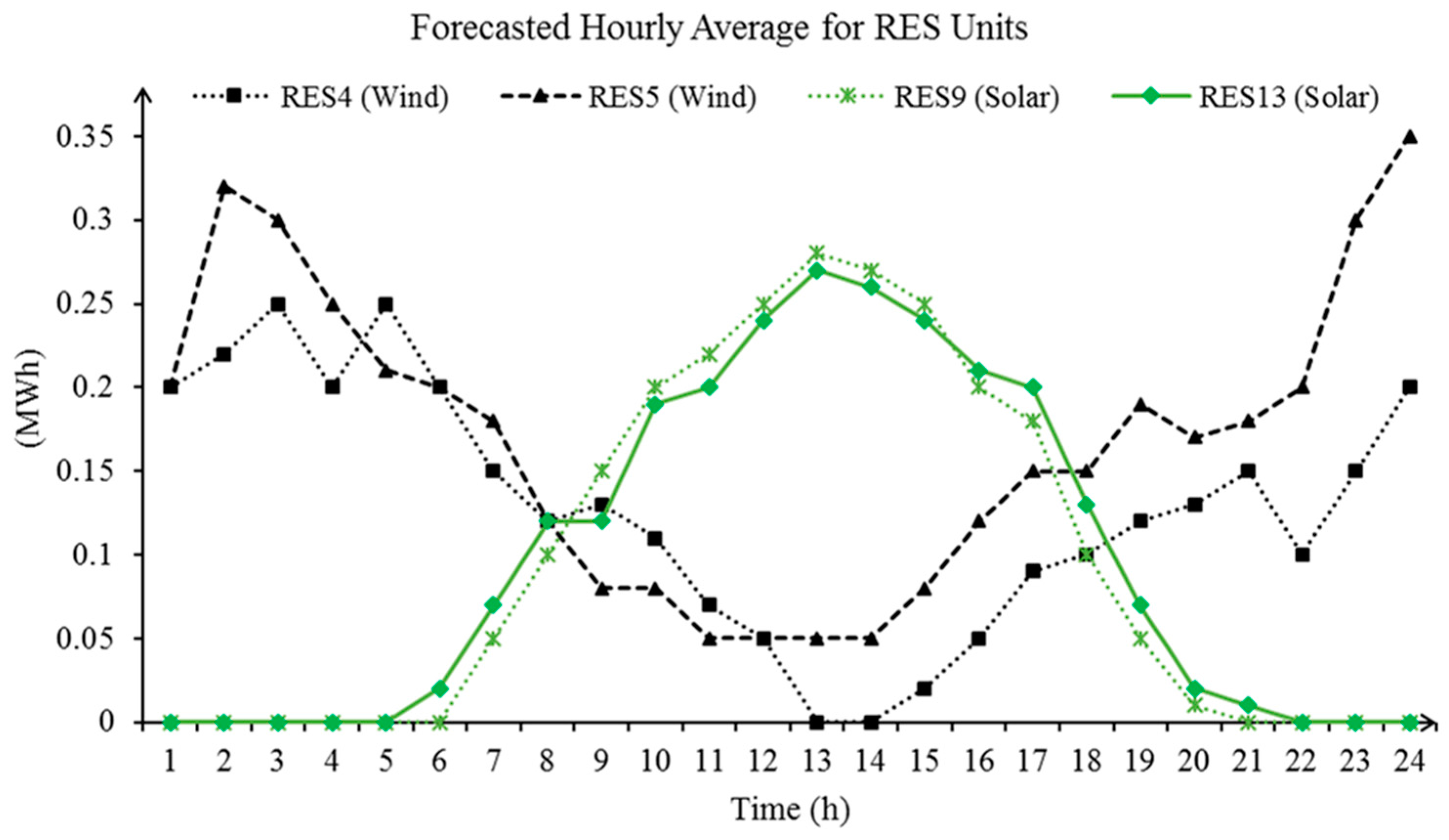
A typical 24-h winter LMP [42], as shown in Figure 4, was used as the bid of the wholesale market. The forecasted hourly generation of the RESs are shown in Figure 5. Due to its non-dispatchable nature, the RES’s generation is considered as a negative fixed load demand and is cleared at DLMP. As seen in Figure 4, the LMP varies from $15/MWh to about $42/MWh. Both EES bids are set to allow charging at 20 $/MWh and discharging at 25 $/MWh. These cost limits are chosen in order to clearly show the charging and discharging schedules of the EES units. Other cost limits can also be applied to the proposed model. Note that a realistic levelized cost of storage (LCOS) constraint should be imposed on the bidding price of the EES units. The LCOS calculation for the EES to participate in the distribution market would account for a number of important factors, including the capital cost, battery degradation, installation labor, operation and maintenance cost, investment tax credit and so on [43]. The calculation of the LCOS is out of the scope of this paper, but the LCOS constraint can be straightforwardly included in the proposed MILP model. EES units charging/discharging bids, as well as its other parameters, are listed in

Table 1. Electrical energy storage (EES) unit parameters.

Bus	Unit	(Min, Max SOC) (MWh)	(Min, Max Power Rate) (MW)	(Min Charge, Discharge Time) (h)	(Injection, ExRaction Cost ($/MWh)	Initial SOC (MWh)
3	EES3	(0.05,0.5)	(0.02,0.05)	(3,3)	(20,25)	0.1
7	EES7	(0.05,0.4)	(0.02,0.05)	(3,3)	(20,25)	0.25

.

The DGs, except DG1, are considered to bid in three blocks. Each block includes a monetary bid and the max amount that the DG can supply at that bid. For DG1, i.e., wholesale injection, only one block with a high supply of 10 MW at LMP is considered. Sample bid blocks of DGs and LAs at 2:00 p.m. are summarized in

Table 2. Energy bids and maximum DG supply (${\mathsf{\delta }}_i^{\mathrm{G}}=\pm 30\%$) for each block at 2:00 p.m.

Bus No, Unit	DG Bids
	Block 1		Block 2		Block 3
	Bid ($/MWh)	Max Supply (MW)	Bid ($/MWh)	Max Supply (MW))	Bid ($/MWh)	Max Supply (MW)
1, DG1	39.80	10	N/A	N/A	N/A	N/A
7, DG7	30.60	1.8	32.40	0.5	35.82	0.5
13, DG13	33.75	0.8	36.72	0.4	39.15	0.3

and

Table 3. LA bid price and maximum demand (${\mathsf{\delta }}_i^{\mathrm{D}}=30\%$) for each block at 2:00 p.m.

Bus No, Unit	LA Bid
	Block 1		Block 2		Block 3
	Bid ($/MWh)	Demand (MW)	Bid ($/MWh)	Demand (MW)	Bid ($/MWh)	Demand (MW)
3, LA3	N/A	0.28	28.05	0.08	23.68	0.10
4, LA4	N/A	0.38	29.29	0.09	23.75	0.17
6, LA6	N/A	0.11	25.25	0.22	20.87	0.16
7, LA7	N/A	0.64	30.38	0.41	25.79	0.48
9, LA9	N/A	0.28	27.91	0.14	21.05	0.17
10, LA10	N/A	0.11	27.66	0.21	22.40	0.18
11, LA11	N/A	0.11	28.79	0.22	23.77	0.28
12, LA12	N/A	0.46	30.73	0.30	25.93	0.19

.

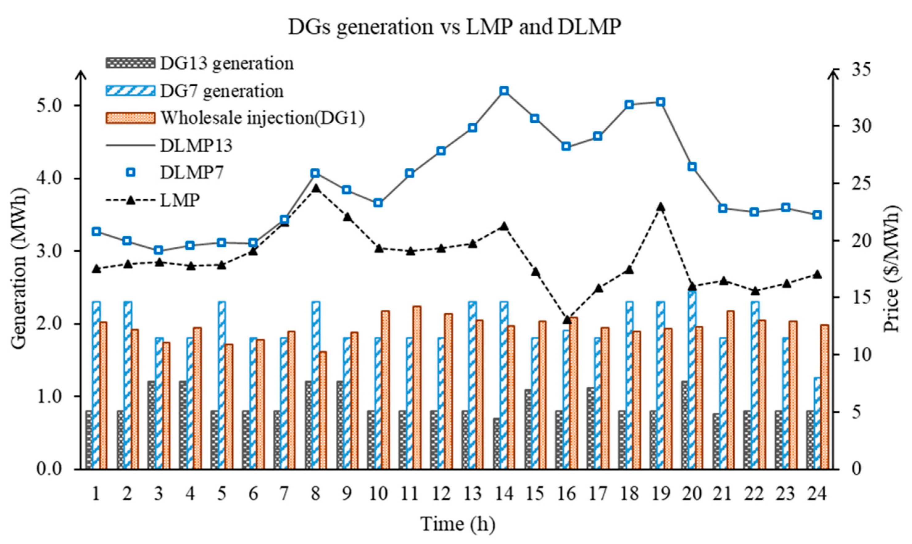
Because of varying LMP throughout the day, DERs and injection from the wholesale market are commissioned at various capacities. As LMP increases, the injection from the wholesale market decreases and the DG’s output increases. This result is depicted in Figure 6 for the DG’s output and the corresponding DLMPs at Buses 1, 7, and 13. DLMPs are calculated by the Lagrange multiplier of the power balance constraint, which shows the marginal price for serving the next MWh at each bus. DLMP 7 and 13 overlap as serving the next increment of load at these buses is equivalent in this case.

As a sample case, the second block bid and the resulting schedule for LA6 versus DLMP at Bus 6 is shown in Figure 7. Note that LAs bid a base load block that needs to be served at all times at DLMP. Figure 7 verifies that only the base load block is scheduled when LA6’s second block bid is lower than the DLMP at Bus 6. The price responsive portion of the LA is only scheduled when its second block bid is higher than the DLMP at that bus.

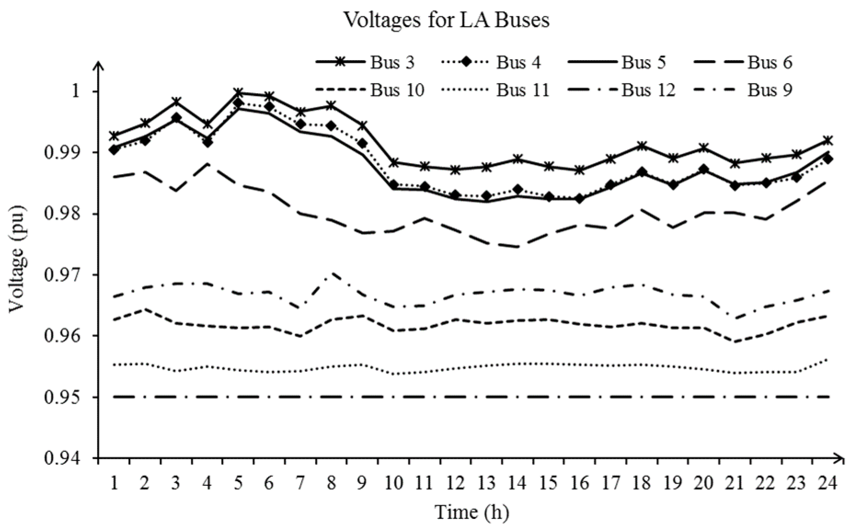
Results of bus voltage magnitudes are within the normal operation limits and are shown in Figure 8 according to the constraint in Equation (8). Notice that buses further away from the substation exhibit higher voltage drops.

The apparent power flow constraint defined in Equation (17) must also be met for all lines. Figure 9 shows the apparent power flow (bars) with respect to the maximum limit for the line from Bus 2 to Bus 3 (horizontal line). Notice that this line hits its maximum limit at hours 13 to 17 and 19 and no further flow is allowed to downstream buses, i.e., Buses 3 and 4. As a result, the DLMPs at Buses 2 and 3 significantly deviate at these hours, as shown in Figure 10. The Lagrange multiplier of the real power flow constraints that reflect the cost of this congestion is activated and is also shown in Figure 10. This verifies that the cost of serving an additional MWh at Bus 3 is higher than that of Bus 2 as no additional power can flow through the lines due to congestion.

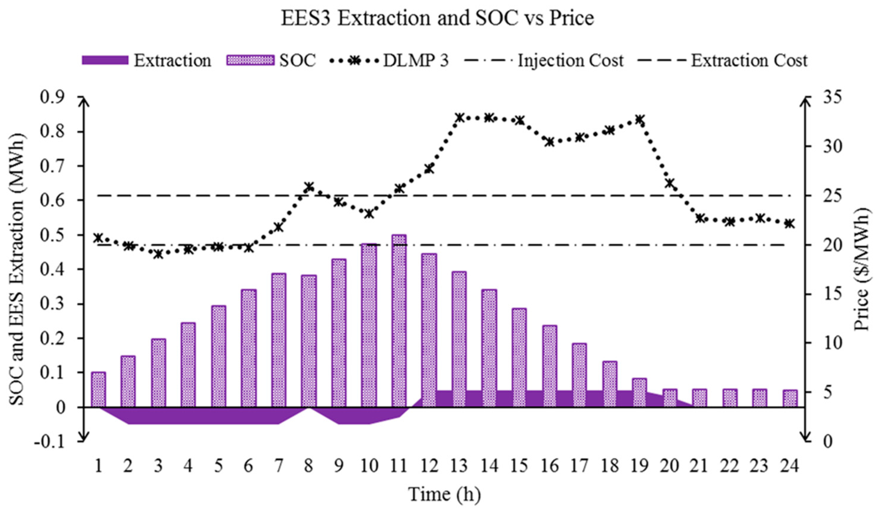
The charge/discharge schedules of the EES units are also dependent on the DLMPs of the buses on which they are located. This result is depicted in Figure 11 and Figure 12 for EES units at Buses 3 and 7 respectively. Here, the dotted graph with markers shows DLMPs and the horizontal lines show the cost of energy injection and extraction of the EES units. The bars and the height of the shaded area show SOC and the amount of energy extraction (charging when negative and discharging when positive) from the EES units respectively. In general, when DLMP is lower than the cost of injection of the EES unit, it is scheduled for charging. Similarly, when DLMP is higher than the cost of extraction, the unit is scheduled for discharging. The SOCs of the units also follow DLMPs, i.e., increase at lower and decrease at higher prices. Note that EES3 at Bus 3 is unable to completely charge until hour 8 since its initial SOC is 0.1 MWh, and the maximum charging rate is 0.05 MW. Furthermore, despite higher DLMPs than the injection cost, it is scheduled for charging during hours 9 to 11. This occurs because DLMPs are much higher later during hours 12 to 20 and it is efficient to charge the unit at slightly higher prices initially, and discharge it at much higher prices later on. This outcome, however, does not ensue in EES7 at Bus 7. This is because the initial SOC of this unit is 0.25 MWh and it is able to fully charge to its maximum limit of 0.4 MWh at lower prices from hours 2 to 7 and discharge during high DLMP from hours 13 to 20.

In Figure 11 and Figure 12, the minimum charging/discharging hours of both EES3 and EES7 were set to 3 consecutive hours. To illustrate the associated constraints, i.e., Equations (23)–(35), are properly met, the minimum charging/discharging hours of EES7 was decreased to 2, and its resulting schedule along with the schedule of EES3 was plotted in Figure 13. In this case, notice that EES7 is allowed an extra cycle of charge/discharge during hours 21 to 24 for further profit, where this schedule change was not possible for the case with 3 minimum charging/discharging hours. The effect of self-discharge can also be seen by the slight slope of SOC of EES7 from hours 6 to 13.

4. Conclusions

In this paper, a detailed MILP model of a DSO’s transactive day-ahead energy auction with high penetration of DERs is proposed. Grid constraints are incorporated in the MILP formulation by use of simplified DistFlow equations. Convex quadratic apparent line flow constraints are linearized using an outer approximation. The proposed model was implemented on a modified IEEE 13-bus system. Simulation results show that the wholesale injection is determined by the LMP at the substation bus. LA’s demand allocation and DG’s supplies are determined by their bids and the DLMP of the bus to which they are connected. When DLMP is lower than the cost of injection of the EES unit, the EES is scheduled for charging. Similarly, when the DLMP is higher than the cost of extraction, the EES is scheduled for discharge. EES units are efficiently scheduled by the DSO while meeting their physical constraints. In our future work, we intend to evaluate and study the effect of bus voltage violations on DLMP and investigate and compare DLMP-based pricing to other administrative valuation approaches such as LMP+D, feed-in tariff, etc. We will also extend this model to its stochastic counterpart to look into how the DSO can efficiently operate the distribution market with uncertainty.

References

- Kristov, L.; De Martini, P.; Taft, J.D. A Tale of Two Visions: Designing a Decentralized Transactive Electric System. IEEE Power Energy Mag. 2016, 14, 63–69. [Google Scholar] [CrossRef]
- Barrager, S.M.; Cazalet, E. A Roadmap toward a Sustainable Business and Regulatory Model: Transactive Energy; 51st State; Baker Street Publishing: San Francisco, CA, USA, 2016; pp. 1–29. [Google Scholar]
- Martini, P.; De Kristov, L. Distribution Systems in a High Distributed Resoures Future: Planning, Market Design, Operation and Oversight; Future Electric Utility Regulation Report No. 2: Berkeley, CA, USA, 2015. [Google Scholar]
- Caramani, M.; Ntakou, E.; Hogan, W.W.; Chakrabortty, A.; Schoene, J. Co-Optimization of Power and Reserves in Dynamic T & D Power Markets With Nondispatchable Renewable Generation and Distributed Energy Resources. Proc. IEEE 2016, 104, 807–836. [Google Scholar]
- Parvania, M.; Fotuhi-Firuzabad, M.; Shahidehpour, M. Optimal demand response aggregation in wholesale electricity markets. IEEE Trans. Smart Grid 2013, 4, 1957–1965. [Google Scholar] [CrossRef]
- Herranz, R.; Muñoz San Roque, A.; Villar, J.; Campos, F.A. Optimal demand-side bidding strategies in electricity spot markets. IEEE Trans. Power Syst. 2012, 27, 1204–1213. [Google Scholar] [CrossRef]
- Wu, D.; Aliprantis, D.C.; Ying, L. Load scheduling and dispatch for aggregators of plug-in electric vehicles. IEEE Trans. Smart Grid 2012, 3, 368–376. [Google Scholar] [CrossRef]
- Sardou, I.G.; Khodayar, M.E.; Khaledian, K.; Soleimani-Damaneh, M.; Ameli, M.T. Energy and reserve market clearing with microgrid aggregators. IEEE Trans. Smart Grid 2015, PP, 1–10. [Google Scholar] [CrossRef]
- Gkatzikis, L.; Koutsopoulos, I.; Salonidis, T. The role of aggregators in smart grid demand response markets. IEEE J. Sel. Areas Commun. 2013, 31, 1247–1257. [Google Scholar] [CrossRef]
- Carlini, E.M.; Sbordone, D.A.; Di Pietra, B.; Devetsikiotis, M. The future interaction between virtual aggregator-TSO-DSO to increase DG penetration. In Proceedings of the International Conference on Smart Grid and Clean Energy Technologies (ICSGCE), Offenburg, Germany, 20–23 October 2015; pp. 201–205. [Google Scholar]
- Faqiry, M.N.; Das, S. Double-Sided Energy Auction in Microgrid: Equilibrium under Price Anticipation. IEEE Access 2016, 4, 3794–3805. [Google Scholar] [CrossRef]
- Zhang, Y.; Gevorgian, V.; Wang, C.; Lei, X.; Chou, E.; Yang, R.; Li, Q.; Jiang, L. Grid-level application of electrical energy storage. IEEE Power Energy Mag. 2017, 15, 51–58. [Google Scholar] [CrossRef]
- Fitzgerald, G.; Mandel, J.; Morris, J.; Touati, H. The Economics of Battery Storage; Rocky Mountain Institute (RMI): Boulder, CO, USA, 2015. [Google Scholar]
- Telaretti, E.; Ippolito, M.; Dusonchet, L. A simple operating strategy of small-scale battery energy storages for energy arbitrage under dynamic pricing tariffs. Energies 2016, 9, 12. [Google Scholar] [CrossRef]
- Rahimi, F.; Mokhtari, S. From ISO to DSO: Imagining new construct--an independent system operator for the distribution network. Public Util. Fortn 2014, 152, 42–50. [Google Scholar]
- Parhizi, S.; Khodaei, A.; Shahidehpour, M. Market-based vs. Price-based Microgrid Optimal Scheduling. In Proceedings of the IEEE International Conference on Smart Grid Communications (SmartGridComm), Miami, FL, USA, 2–5 Novermber 2015; pp. 1–9. [Google Scholar] [CrossRef]
- Wu, H.; Shahidehpour, M.; Khodayar, M.E. Hourly demand response in day-ahead scheduling considering generating unit ramping cost. IEEE Trans. Power Syst. 2013, 28, 2446–2454. [Google Scholar] [CrossRef]
- Faqiry, M.N.; Zarabie, A.K.; Nassery, F.; Wu, H.; Das, S. A Day Ahead Market Energy Auction for Distribution System Operation. In Proceedings of the IEEE Conference on Electro-Information Technology, Lincoln, NE, USA, 14–17 May 2017; pp. 1–6. [Google Scholar]
- Baringo, L.; Conejo, A.J. Offering Strategy of Wind-Power Producer: A Multi-Stage Risk-Constrained Approach. IEEE Trans. Power Syst. 2016, 31, 1420–1429. [Google Scholar] [CrossRef]
- Baringo, L.; Conejo, A.J. Strategic offering for a wind power producer. IEEE Trans. Power Syst. 2013, 28, 4645–4654. [Google Scholar] [CrossRef]
- Baillo, A.; Cerisola, S.; Fernandez-Lopez, J.M.; Bellido, R. Strategic bidding in electricity spot markets under uncertainty: A roadmap. In Proceedings of the IEEE Power Engineering Society General Meeting, Montreal, QC, Canada, 18–22 June 2006. [Google Scholar] [CrossRef]
- Sotkiewicz, P.M.; Vignolo, J.M. Nodal pricing for distribution networks: Efficient pricing for efficiency enhancing DG. IEEE Trans. Power Syst. 2006, 21, 1013–1014. [Google Scholar] [CrossRef]
- Verzijlbergh, R.A.; De Vries, L.J.; Lukszo, Z. Renewable Energy Sources and Responsive Demand. Do We Need Congestion Management in the Distribution Grid? Power Syst. IEEE Trans. 2014, 29, 2119–2128. [Google Scholar] [CrossRef]
- Liu, Z.; Wu, Q.; Oren, S.; Huang, S.; Li, R.; Cheng, L. Distribution Locational Marginal Pricing for Optimal Electric Vehicle Charging through Chance Constrained Mixed-Integer Programming. IEEE Trans. Smart Grid 2016, PP, 1. [Google Scholar] [CrossRef]
- O’Connell, N.; Wu, Q.; Østergaard, J.; Nielsen, A.H.; Cha, S.T.; Ding, Y. Day-ahead tariffs for the alleviation of distribution grid congestion from electric vehicles. Electr. Power Syst. Res. 2012, 92, 106–114. [Google Scholar] [CrossRef] [Green Version]
- Kristoffersen, T.K.; Capion, K.; Meibom, P. Optimal charging of electric drive vehicles in a market environment. Appl. Energy 2011, 88, 1940–1948. [Google Scholar] [CrossRef]
- Faqiry, M.N.; Sanjoy, D. Distributed Bi-level Energy Allocation Mechanism with Grid Constraints and Hidden User Information. arXiv, 2017; arXiv:1707.05429. [Google Scholar]
- Wu, H.; Shahidehpour, M.; Alabdulwahab, A.S.; Abusorrah, A. A Game Theoretic Approach to Risk-Based Optimal Bidding Strategies for Electric Vehicle Aggregators in Electricity Markets With. IEEE Trans. Sustain. Energy 2016, 7, 374–385. [Google Scholar] [CrossRef]
- Wu, F.F. Network reconfiguration in distribution systems for loss reduction and load balancing. IEEE Trans. Power Deliv. 1989, 4, 1401–1407. [Google Scholar]
- Baran, M.E.; Wu, F.F. Optimal sizing of capacitors placed on a radial distribution system. IEEE Trans. Power Deliv. 1989, 4, 735–743. [Google Scholar] [CrossRef]
- Yeh, H.; Member, S.; Gayme, D.F.; Low, S.H. Adaptive VAR Control for Distribution Circuits With Photovoltaic Generators. IEEE Trans. Power Syst. 2012, 27, 1656–1663. [Google Scholar] [CrossRef]
- Wang, Z.; Chen, B.; Wang, J.; Kim, J. Decentralized Energy Management System for Networked Microgrids in Grid-Connected and Islanded Modes. IEEE Trans. Smart Grid 2016, 7, 1097–1105. [Google Scholar] [CrossRef]
- Turitsyn, K.; Šulc, P.; Backhaus, S.; Chertkov, M. Distributed control of reactive power flow in a radial distribution circuit with high photovoltaic penetration. In Proceedings of the IEEE PES General Meeting, Providence, RI, USA, 25–29 July 2010. [Google Scholar]
- Lamont, J.W.; Fu, J. Cost analysis of reactive power support. IEEE Trans. Power Syst. 1999, 14, 890–898. [Google Scholar] [CrossRef]
- Bhattacharya, K.; Zhong, J. Reactive power as an ancillary service. IEEE Trans. Power Syst. 2001, 16, 294–300. [Google Scholar] [CrossRef]
- Kahn, E.; Baldick, R. Reactive Power is a Cheap Constraint. Int. Assoc. Energy Econ. 2017, 15, 191–201. [Google Scholar]
- Taylor, J.A. Convex Optimization of Power Systems; Cambridge University Press: Cambridge, UK, 2015; ISBN 978110707687. [Google Scholar]
- Divya, K.C.; Østergaard, J. Battery energy storage technology for power systems—An overview. Electr. Power Syst. Res. 2009, 79, 511–520. [Google Scholar] [CrossRef]
- Fitzgerald, G.; Mandel, J.; Morris, J.; Touati, H. The Economics of Battery Energy Storage: How Multi-Use, Customer-Sted Batteries Deliver the Most Services and Value to Customers and the Grid; Rocky Mountain Institute: Boulder, CO, USA, 2015; p. 41. [Google Scholar]
- He, G.; Chen, Q.; Kang, C.; Pinson, P.; Xia, Q. Optimal Bidding Strategy of Battery Storage in Power Markets Considering Performance-Based Regulation and Battery Cycle Life. IEEE Trans. Smart Grid 2016, 7, 2359–2367. [Google Scholar] [CrossRef]
- GAMS Development Corporation. General Algebraic Modeling System (GAMS) Release 24.7.4.; GAMS Development Corporation: Washington, DC, USA, 2016. [Google Scholar]
- SPP Locational Marginal Price. Available online: https://marketplace.spp.org/pages/rtbm-lmp-by-location (accessed on 8 October 2017).
- DiOrio, N.; Dobos, A.; Janzou, S. Economic Analysis Case Studies of Battery Energy Storage with SAM; National Renewable Energy Laboratory: Denver, CO, USA, 2015.
Figure 1.
Piecewise traditional supply-demand curve with supply blocks labeled ‘q’, demand blocks labeled ‘r’, and prices labeled ‘cr’ and ‘cq’. Demand curve is shifted due to LA’s base load block (r1).
Figure 2.
Radial IEEE 13-bus distribution system with different types of distributed energy resources (DERs) on each bus.
Figure 3.
Schematic diagram of single branch radial distribution system with N nodes.
Figure 4.
Realistic locational marginal price (LMP) values for different seasons.
Figure 5.
Wind and Solar forecasted hourly average generation.
Figure 6.
Wholesale injection at LMP versus DG7 and DG13’s schedules and DLMPs.
Figure 7.
LA6 bid versus DLMP at Bus 6 and its schedule.
Figure 8.
Voltage magnitudes for LA buses.
Figure 9.
Apparent power flow in Line 2–3 demonstrating line limits are not exceeded.
Figure 10.
DLMP at Bus 2, 3, and the effect of congestion at Line 2–3.
Figure 11.
EES3’s schedule is dependent upon the DLMP at Bus 3.
Figure 12.
EES7’s schedule is dependent upon the DLMP at Bus 7.
Figure 13.
EES injection/extraction with 2-h minimum charging/discharging constraint.