Modeling and Control of Fluid Flow Networks with Application to a Nuclear-Solar Hybrid Plant


Institute of Nuclear and New Energy Technology, Collaborative Innovation Centre of Advanced Nuclear Energy Technology, Key Laboratory of Advanced Reactor Engineering and Safety of Ministry of Education, Tsinghua University, Beijing 100084, China
*
Author to whom correspondence should be addressed.
Energies 2017, 10(11), 1912; https://doi.org/10.3390/en10111912
Submission received: 1 November 2017
/
Revised: 13 November 2017
/
Accepted: 18 November 2017
/
Published: 20 November 2017
(This article belongs to the Special Issue The Future of Solar Thermal Energy)
Abstract
:Fluid flow networks (FFNs) can be utilized to integrate multiple once-through heat supply system (OTHSS) modules based on either the same or different energy resources such as the renewable, nuclear and fossil for multi-modular and hybrid energy systems. Modeling and control is very important for the safe, stable and efficient operation of the FFNs, whose objective is to maintain both the flowrates and pressure-drops of the network branches within specific bounds. In this paper, a differential-algebraic nonlinear dynamic model for general FFNs with multiple pump branches is proposed based on both the branch hydraulics and network graph properties. Then, an adaptive decentralized FFN flowrate-pressure control law, which takes a proportional-integral (PI) form with saturation on the integral terms, is established. This newly-built control not only guarantees satisfactory closed-loop global stability but also has no need for the values of network hydraulic parameters. This adaptive control is then applied to the flowrate-pressure regulation of the secondary FFN of a two-modular nuclear-solar hybrid energy system and numerical simulation results show the feasibility and high performance of this network control strategy. Due to its concise form, this new flowrate-pressure FFN controller can be easily implemented practically.
1. Introduction
Distributed energy systems can be built by electrical interconnection of power plants through the grid [1] and can also be built by thermal interconnection [2] of homogeneous or heterogeneous once-through heat supply system (OTHSS) modules based on fluid flow networks (FFNs). As shown in Figure 1, OTHSS refers to a thermodynamic system composed of a heat source, primary coolant circuit(s) and once-through steam generator(s) (OTSG) or once-through heat exchanger(s) (OTHX), whose heat source can be fired-coal, nuclear fission reaction, solar and etc. The coolant inside the primary circuits is used to absorb the heat from the source and transfers it to the secondary coolant through OTSGs or OTHXs. The secondary coolant is injected to the secondary side of the OTSGs or OTHXs and is changed to be the satisfactory working fluid for driving different thermal loads such as a steam turbine. Actually, OTHSS are very common in practical engineering such as the integral pressurized water reactors (iPWR, e.g., Nuscale, IRIS and mPower) with internal OTSGs [3,4,5,6], modular high temperature gas-cooled reactor (MHTGR, e.g., HTR-Module [7,8,9], MHTGR [10] and HTR-PM [11,12,13]) with side-by-side arranged OTSGs, concentrating solar power (CSP) plants with OTSGs [14] or OTHXs [15] and even coal-fired once-through boilers. A thermally interconnected distributed energy system is called a hybrid energy system (HES) [16,17,18] if the heat sources of OTHSS modules are of different types, otherwise it is called a multimodular energy system.
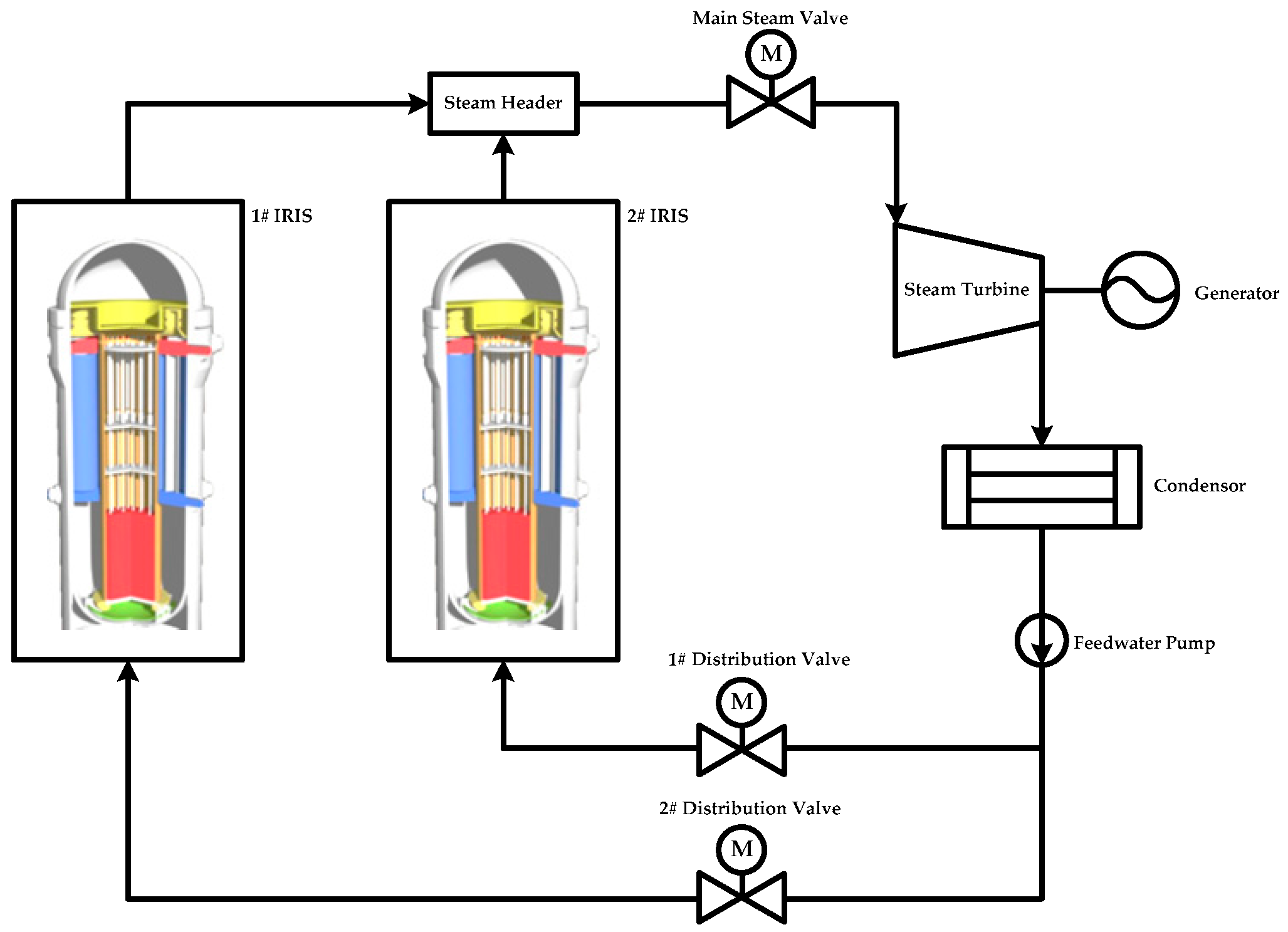
FFNs can be used to build multimodular nuclear plants based on small modular reactor (SMRs) which are defined to be those fission reactors with electric power no more than 300 MWe. Figure 2 illustrates the schematic diagram of a two-modular IRIS-based nuclear plant [19], where the live superheated steam flows of 331 °C/5.8 MPa provided by the two IRIS-based nuclear steam supply system (NSSS) modules are combined together to drive the turbine and the condensed water are then pressurized by the feedwater pump and distributed to each IRIS module by the valves. The secondary-side of the fluid flow network (FFN) that interconnects these two IRIS modules of the plant is shown by Figure 3a, where branch f is the pump branch including the feedwater pump, branch i is the secondary side of the ith IRIS module (i = 1, 2) and branch 3 composes of the equipment such as the turbine, condenser, deaerator, etc. Similarly, m-modular IRIS plant can be realized by the parallel operation of m IRIS module through feedwater distribution and steam combination and the corresponding secondary FFN is illustrated by Figure 3b. Moreover, Figure 4 shows the simplified diagram of a two-modular MHTGR-based nuclear plant HTR-PM which is under construction at China, Shandong Shidao bay, where the NSSS module is mainly constituted by a pebble-bed MHTGR, a primary helium blower and a side-by-side arranged OTSG, each NSSS module is independently equipped with a feedwater pump and the live steam flows from multiple modules and with the parameters of 571 °C/13.9 MPa are combined to drive the turbine [13]. The secondary FFN of HTR-PM plant is shown by Figure 5a and the FFN corresponding to the m-modular MHTGR plant with independent feedwater strategy is shown by Figure 5b [20]. From Figure 2, Figure 3, Figure 4 and Figure 5, if the live steam parameters of different NSSS modules are identical, then these modules can be integrated by parallel operation, based on which the strong safety feature of SMRs can be applicable to large-scale nuclear plants at any desired power ratings.
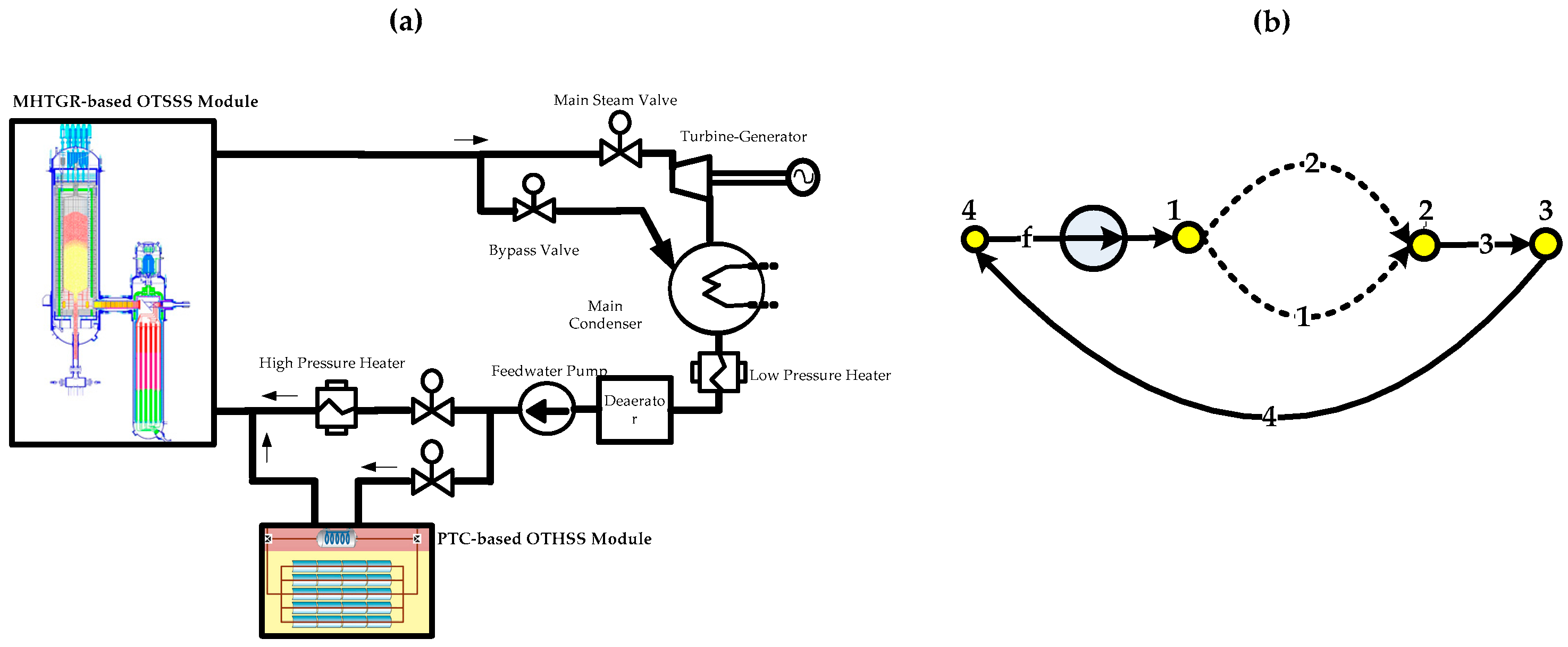
Moreover, FFNs can also be applied to build nuclear-solar HESs by integrating the OTSSS modules based on NSSS and CSP. For CSP modules, the parabolic through collector (PTC) system and solar power tower (SPT) system are two significant types [21]. The PTC system consists of a group of reflectors that are curved in on dimension in parabolic shape to focus sunrays onto an absorber tube mounted in the focal line of the parabola. The SPT system uses a field of heliostats to reflect and concentrate the sunrays onto a central receiver placed in the top of a fixed tower. Both the PTC and SPT systems can power a secondary steam circuit and Rankine power cycle. Based on the secondary FFN given by Figure 3 or Figure 5, e.g., the SPT-based OTSSS proposed in [12] can be integrated in parallel with the MHTGR-based OTSSS introduced in [13] to realize a HES shown in Figure 6 if the live steam parameters of these heterogeneous OTSSS modules are identical. Furthermore, a nuclear-solar HES can also be realized by serial integration of different modules, e.g., Figure 7 gives the schematic diagram of a serially integrated HES [13], where a PTC-based OTHSS is adopted to heat up the feedwater flow of a MHTGR-based NSSS module in parallel with a high-pressure heater (HPH). Here, in Figure 7b, branch f is the pump branch including the feedwater pump, branch 1 contains the original HPH, branch 2 is the secondary side of the PTC-based module, branch 3 is the secondary side of the OTSG of the MHTGR-based module and branch 4 composes of the equipment such as the turbine, condenser, deaerator and etc. Through the heterogeneous integration scheme shown by Figure 7, there is less necessity of storage devices with large capacity for the CSP-module, which leads to system simplification and cost reduction. Moreover, there is higher steam parameters, which induces better turbine efficiency. Therefore, based on the above introduction as well as the instances shown in Figure 2, Figure 3, Figure 4, Figure 5, Figure 6 and Figure 7, FFN is central in thermally integrating homogeneous or heterogeneous OTHSS modules with parallel, serial and some other integration manners.
Based on the above discussion, to guarantee the stable and efficient operation of multi-modular or hybrid energy systems, it is basically needed to drive the flowrates and (or) pressure-drops of their secondary FFN to their desired values. To achieve this objective, it is crucial to give a proper FFN control law which is the mechanism of adjusting the resistances of network branches and (or) the pressure-heads of pumps or blowers by changing the valve openings and (or) the rotation speeds of pumps/blowers. FFN control method was studied since1970s [22,23,24,25]. In [25], a FFN flowrate controller was proposed by Kocić based on the linearized model of a mine ventilation network, which however cannot handle the network nonlinearity. After 2000, some important progresses in FFN control have been made [26,27,28]. By incorporating the branch fluid dynamics and network graph features, the non-mininal and minimal models for FFNs with single pump were proposed and two centralized flowrate controllers, which need the flowrate measurements of all the network branches, were also given [26]. By analyzing the dissipativity of FFN with a single pump, Dong proposed a decentralized flowrate controller that not only guarantees globally asymptotic stability (GAS) but also takes the simple proportional-integral (PI) form [27]. By giving a nonlinear differential-algebraic model for FFN with a single pump, a flowrate-pressure controller providing globally bounded stability was proposed in [28] and was then applied for realizing module coordination control of multi-modular nuclear plants integrated by the feedwater distribution scheme shown in Figure 3.
However, there is still no result in the dynamic modelling and flowrate-pressure control of general FFNs with multiple pumps or blowers, which is crucial in building multi-modular and hybrid energy systems based on integrating multiple OTHSS modules. In this paper, a nonlinear differential-algebraic model for FFNs with multiple pumps is proposed based on the branch dynamics and network graph property. Then, a novel adaptive decentralized flowrate-pressure controller is given for FNNs with a simple form. Finally, this newly-built control law is applied to realize the flowrate-pressure regulation for a FFN utilized to realize a two-modular nuclear-solar hybrid energy system (HES) and numerical simulation results show the feasibility and satisfactory performance of this newly-built FFN control. The novelty of this paper lies on two aspects, where the first one is to convert the control problem of hybrid and multimodular energy system to the control problem of FFNs and the second one is the modeling and flowrate-pressure control design for fluid flow networks.
2. Nonlinear Differential-Algebraic Model
Suppose that there are n branches without pump, m fan branches and nc nodes in a FFN, where each fan branch has a single fan or pump. In this section, the branch dynamics and graph properties of a FFN are introduced and then a differential-algebraic model describing the FFN dynamics is given.
2.1. Branch Dynamics
Based on the conservation law of momentum, the fluid motion in the branches without pump can be written as [29]:
where = [Q1, …, Qn]T, = diag(Q1|Q1|, …, Qn|Qn|), K = diag(K1, …, Kn), R = [R1, …, Rn]T, H = [H1, …, Hn]T and scalars Qj, Rj, Hj and Kj is respectively the flowrate, dynamic resistance, pressure drop and inertia coefficient of branch j (j = 1, …, n).
2.2. Graph Properties
Assume that node i is connected to the fan branch i (i = 1, …, m). The fluid flow network can be divided in to a tree containing the fan branches and its complement, i.e., the co-tree whose branches are referred to as the links. The number of links is [30]:
From Kirchhoff’s voltage law (KVL) [30],
where Hf = [Hfj]m×1, EH = [EHij](l-k)×n, eHf = [eHfij]k×n, ΓHf = [λHfij]k×m, k is the number of fundamental loops containing the fan branches, Hfj (j = 1, …, m) is the pressure drop of pump branch j. If branch j (j = 1, …, n) is contained in fundamental loop (FL) i (i = 1, …, k) with the same (opposite) direction, then EHij = 1(−1), else EHij = 0. If branch j (j = 1, …, n) is in FL l – k + i (i = 1, …, k) with the same (opposite) direction, then eHfij = 1(−1), else eHfij = 0. Moreover, if fan branch j (j = 1, …, m) is in FL l − k + i with the same (opposite) direction, then λHfij = 1(−1), else λHfij = 0. Here, Hf can be further expressed as
where Hd = [Hdj]m×1, Rf = diag(Rf1, …, Rfn), Qf = [Qfj]m×1, Hdj is the pressure head provided by fan (or pump) j, Qfj is the flowrate of pump branch j and Rfj is the resistance coefficient of pump branch j (j = 1, …, m).
From Kirchhoff’s current law (KCL) [30],
where EQ = [EQij](nc-m-1)×n, eQf = [eQfij]m×n, ΓQf = [λQfij]m×m. If branch j (j = 1, …, n) is connected to node i + m (i = 1, …, nc − m − 1) with flow going away (into) from node i + m, then EQij = 1(−1), else EQij = 0. If branch j (j = 1, …, n) is connected to node i + 1 with flow going into node i + m, EQij = 0 if branch j is not connected to node i + m. If branch j is connected to node i (i = 1, …, m) with flow going into (away from) the node, then eQfij = 1(−1), else eQfij = 0. If fan branch j is connected to node i (i = 1, …, m) with flow going into (away from the node, λQfij = 1(−1), else λQfij = 0.
2.3. Differential-Algebraic Network Model
It is not loss of generality to make the following assumptions:
- (A1)
- Branches 1 to l correspond to the links.
- (A2)
- Branches l + 1 to n + m correspond to tree-branches and all the fan branches are in the tree.
From assumptions (A1) and (A2) as well as Equations (3) and (5),
where Hc = [H1, …, Hl]T, Ha = [Hl+1, …, Hn]T, Qc = [Q1, …, Ql]T, Qa = [Ql+1, …, Qn]T.
Then, based on the duality of KVL and KCL [30] and by choosing
EQa = Inc−m−1, ΓQf = Im, eQfa = Om×(nc−m−1), i.e.,
we have
From Equation (10),
From Equation (7),
From Equations (3), (4), (8) and (11), we can derive that
where
By substituting (14) with
we have
Since EQ is a constant matrix, from Equation (5),
Substitute (1) to (18),
Then from (14) and (19), we can obtain that
The above analysis and derivation can be summarized as following Proposition 1.
Proposition 1.
The dynamics of fluid flow networks with multiple pumps can be expressed by differential-algebraic model
Remark 1.
From model (21), FFN dynamical behavior is given by branch hydraulic parameters Rfj (j = 1, …, m) and Ki (i = 1, …, n) as well as network topological matrices EQc and eQfc.
3. Flowrate-Pressure Control Design
3.1. State-Space Model
Define
From Equations(16), (22) and (23),
Suppose the referenced values (setpoints) of Qc, Qa, Rcc, Ra and Hd are constant vectors Qcr, Qar, Rccr, Rar and Hdr respectively. Define Qce = Qc − Qcr, Qae = Qa − Qar, Rcce = Rcc − Rccr, Rae = Ra − Rar, Hde = Hd − Hdr, where it can be seen from (13) that Qae = −EQcQce. Here, Rcc, Ra and Hd are chosen as the control input to regulate the branch flowrates and pressure-drops.
Then, the state-space model for control design can be expressed as
where
and matrices Ωc and Ωa are all positive-definite.
3.2. Globally Asymptotic Control Design
Choose the Lyapunov function as
which represents the variation of kinetic energy stored in the FFN. Differentiate V1 along the trajectory given by model (25),
Moreover, from the second equation of model (25),
Through adding (27) and (28), we have
Design Hde, Rcce and Rae as
respectively, where constant matrices Γd, Γcc and Γa are all positive-definite. Then, substitute (30)–(32) to (29),
where
From Equation (33), if matrix inequality
is well satisfied, then
i.e., the closed-loop is globally asymptotically stable. The above control design can be summarized as the following Proposition 2.
Proposition 2.
Consider nonlinear differential-algebraic system (25) with the control input
Then, the closed-loop system globally asymptotically stable if matrix Inequality (36) is well satisfied.
Remark 2.
Usually, due to the network parameter uncertainty, referenced vectors Hdr, Rccr and Rar are very hard to be obtained, which means that control laws (38)–(40) cannot be implemented in practical engineering. Therefore, it is necessary to design adaptive laws for the estimation of these parameters. Since Hdr, Rccr and Rar related to the practical feedwater headers and valve openings, it is reasonable to assume that they are norm-bounded, i.e.,
where Hdrm, Rccrm and Rarm are all given positive constants.
3.3. Adaptive Control Design
According to (38)–(40), choose the control input as
where , and are estimations of Hdr, Rccr and Rar respectively.
In order to design the adaptation laws for estimation , and , choose the extended LyaPunov function as
where , , and constant diagonal matrices Ξd, Ξcc and Ξa are all positive-definite. Differentiate V2 along the closed-loop trajectory given by model (25) and control inputs (44)–(46),
Design the adaptation laws as
where function proj(∙) is defined by
with scalar given by
From (41)–(43), (52) and (53), estimation , and as well as estimation error , and are all bounded.
Then, by substituting (49)–(51) to (48), if matrix inequality
is well satisfied, where Γe is an arbitrarily given positive-definite matrix and Πa is given by equation (35), then
which means that the closed-loop system is globally bounded stable.
The above adaptive control design can be summarized as the following Proposition 3.
Proposition 3.
Consider nonlinear differential-algebraic system (25) with adaptive flowrate-pressure control given by
If Inequality (54) holds, then the closed-loop constituted by model (21) and adaptive control (56) is globally bounded stable.
Remark 3.
From (56), the flowrate-pressure control law can be rewritten as
which takes form of proportional-integral (PI) feedback laws.
Remark 4.
Moreover, the tuning method of FFN flowrate-pressure control law is determined from the design process given before Proposition 3. From inequality of (55) and (54) as well as Equation (35), the entries of diagonal positive-definite matrices Γd, Γc and Γa is larger, the speed of function V2 converging to the origin is faster, which means that the errors of the flowrates and pressures decrease faster. Moreover, the function of positive matrices Ξd, Ξcc and Ξa is to make the steady control errors of flowrates and pressures to be zero.
Remark 5.
The pressure-drop can be measured by the sensors such as elastic pressure gauge and membranometer, which depends on the scope of FFN operation pressure. The flowrate can be measured by difference pressure flow meter. Moreover, from Equation (57), flowrate-pressure control law are decentralized, which means that each flowrate or pressure control input only needs the measurement of the process variable regulated by this control input.
4. Application to a Nuclear-Solar Hybrid Plant
4.1. Feasibility of HES Based on MHTGR and STP
Due to the demand of clean renewable electric power, a number of CSP plant are being considered for deployment around the world. It has been pointed out by International Energy Agency (IEA) that CSP could provide 11.3% of global electricity by 2050. As introduced in Section 1, SPT plant is an important type of CSP plant and is also known as central receiver system. A SPT uses a heliostat field collector (HFC), i.e., a field of sun tracking reflectors called heliostat that reflect and concentrate the sunrays onto a central receiver placed in the top of a fixed tower. In the central receiver, heat is absorbed by a heat transfer fluid (HTF) such as the widely adopted molten salt, which then transfers heat to power a steam Rankine cycle. Relative to PTC, SPT achieves very high temperatures, which can increase the efficiency of conversion from heat to electricity and can also reduce the cost of thermal storage. Additionally, the piping system is concentrated in the central area of a SPT plant, which reduces the related energy losses, material costs and maintenance [31].
STPs with or without thermal storage are commonly equipped with a fuel backup system (BS) that helps to regulate production and to guarantee a nearly constant generation capacity. The integration of STP and BS modules can further reduce investments in reserving solar field and storage capacity [21,31]. Nowadays, the BS modules are usually realized through burning fossil fuels. Actually, since nuclear fission is a crucial clean base-load energy source that can substitute the fossil in a centralized way and in a great amount, it can be adopted for building the BS module of a STP, which induces the realization of nuclear-solar HESs with the virtue of persistent power supply. However, it is necessary to find the nuclear reactors with the ability of generating superheated steam, which can be coupled with STPs for building thermally coupled nuclear-solar HESs. Actually, modular high temperature gas-cooled reactor (MHTGR), which uses helium as the coolant and graphite as both the moderator and structure material, is a suitable fission reactor for building nuclear superheated steam supply system (Su-NSSS) modules that can be adopted as the BS of STP modules for realizing nuclear-solar hybrid plants.
The nuclear-solar HES composed of STP-based and MHTGR-based OTSSSs is a clean energy system fully free from carbon-emission. Due to its low power density, strong temperature negative feedback effect and large surface-to-volume ratio, MHTGR has the crucial inherent safety feature, which induces the simplification of safety-related systems and the reduction in reactor maintenance and leads to the feasibility of building MHTGR-STP coupled HES near large load centers. Moreover, since the primary coolant of MHTGR is helium and due to the high thermal efficiency of both MHTGR-based and SPT-based OTSSSs that induced by high live steam temperature, the water requirement of MHTGR-STP coupled HES should be lower than the pressurized water reactor (PWR) nuclear plant, PTC plant and their coupled HESs, which leads to the feasibility of building MHTGR-STP coupled HESs for the locations with water scarcity. Based on the above discussion, it can be seen that nuclear-solar HESs constituted by MHTGR-based and STP-based OTSSSs has the virtues of inherent nuclear safety, high thermal efficiency and low cost of construction and maintenance, which shows the strong feasibility of its deployment.
4.2. A MHTGR-STP Coupled HES
4.2.1. Schematic Diagram and Design Parameters
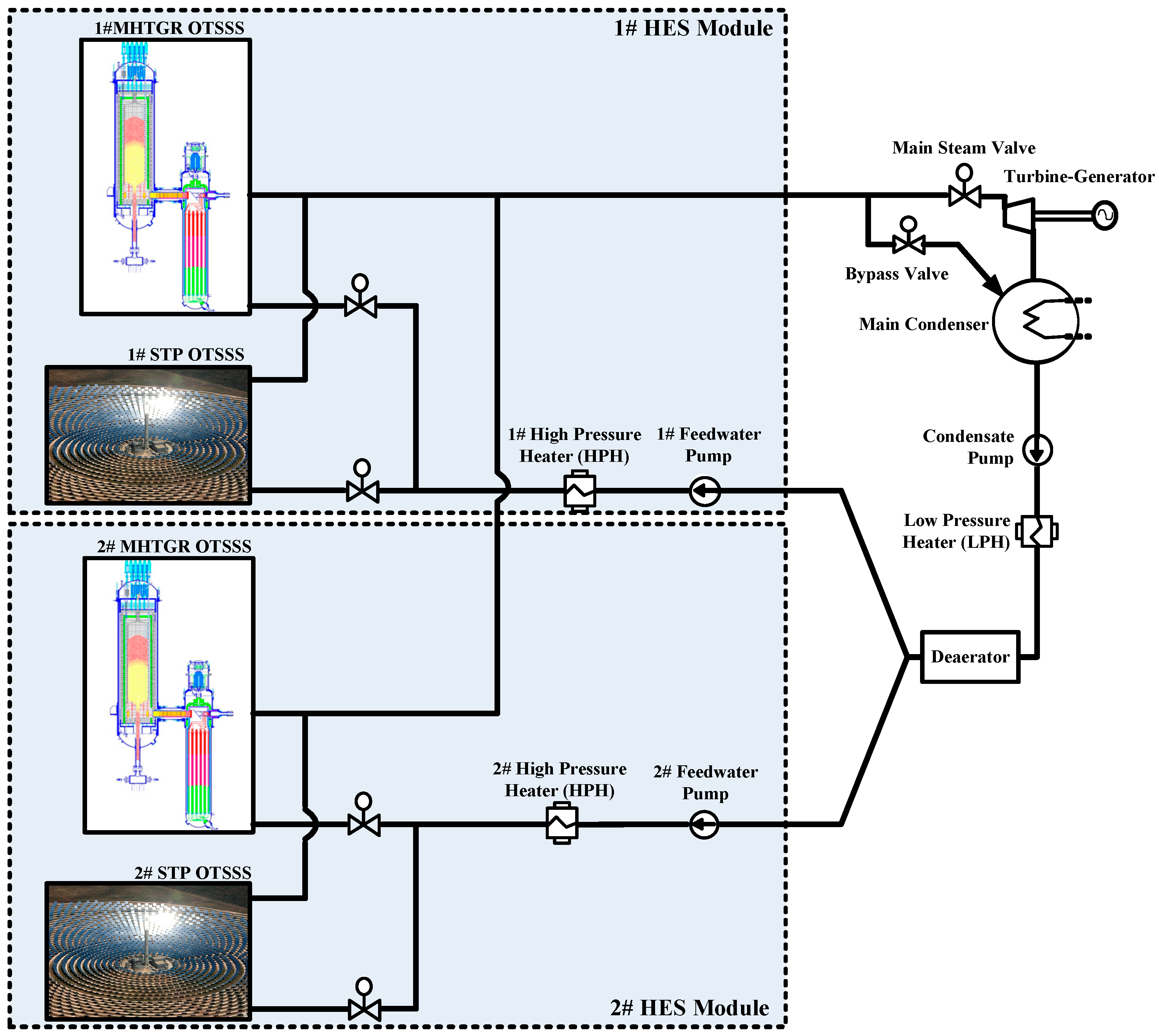
Figure 8 gives a schematic diagram of a nuclear-solar HES having two superheated steam supply system (4S) modules operating in parallel. Every 4S module is composed of a STP-based OTSSS and an MHTGR-based OTSSS and is independently equipped with a feedwater pump as well as a high-pressure heater (HPH). Moreover, for a 4S module, the feedwater is distributed to the MHTGR- based and STP-based OTSSSs of this module through adjusting the opening of governing valves. For the STP-based OTSSS, the molten salt is heated up in the central receiver to a high temperature by absorbing solar energy and transfers the heat to the feedwater for superheated steam production. For the MHTGR-based OTSSS, the cold helium is injected by the primary blower into the reactor core where it is heated up to a high temperature and flows to the primary-side of helical-coil OTSG where it turns the feedwater to superheated steam. The superheated live steam flows generated by the STP-based and MHTGR-based OTSSSs belonging to the two 4S modules are combined together to drive the turbine/generator set for electricity production. The condensed water is pressurized by the condensate pump and heated up by the low-pressure heater (LPH) successively and then flows into the deaerator. The water inside the common deaerator is fed to a 4S module by its feedwater pump and the feedwater is further heated up by the HPH before being distributed to the two OTSSSs in the same module for a new cycle. The designed values of the main parameters of MHTGR-based and STP-based OTSSSs at rated condition are given in Table 1 [13,32,33], where the main design parameters of the STP is computed based on [32,33].
4.2.2. Secondary FFN and Control Strategy
Moreover, the secondary FFN of this two-modular nuclear-solar HES is shown in Figure 9, where branches f1 and f2 are the pump branches including the feedwater pump and high pressure heater (HPH), branch 2i − 1 is the secondary side of the ith MHTGR-based OTSSS (i = 1, 2), branch 2i is the secondary side of the ith STP-based OTSSS (i = 1, 2) and branch 5 composes of the equipment such as the turbine, condenser, low pressure heater (LPH) and deaerator. Since the realization and stable operation of the two-modular nuclear-solar HES shown in Figure 9 heavily depends on the condition that the pressure of the live steam flows generated by different OTSSSs of the two modules should be identical in both steady and transient states, it is necessary to regulate the OTSSS flowrates and main steam pressure, which are just the flowrates of branch i (i = 1, …, 4) and pressure-drops of branch 5 of the secondary FFN shown in Figure 9 respectively. Here, the newly-built adaptive flowrate-pressure control law (57) is applied to solve this FFN regulation problem, where header Hd adjusted by the rotation speed of pumps is utilized to regulate the flowrates of branches 1 and 2, resistance Rcc adjusted by the opening of feedwater valves in branches 3 and 4 is utilized to regulate the corresponding flowrates and resistance Ra adjusted by the steam valve opening is utilized to regulate the main steam pressure.
4.3. Simulation Results with Discussions
4.3.1. Controller Parameters
For the FFN given by Figure 9, it can be seen that nc = 4, m = 2, n = 5, l = 4 and topology matrices EQc and eQfc are given by
respectively. In this simulation, the network parameters are chosen to be Ki = 0.1 (kg/MPa∙s2) (i = 1, …, 5), R1 = R2 = 0.006 MPa/(kg/s)2, Rf1 = Rf2 = 0.0001 MPa/(kg/s)2 and the parameters FFN pressure-flowrate controller (56) are set to be Γd = 0.5I2, Πd = 100 I2, , Γcc = 0.05 , Πcc = 200 , , Γa = 0.01 , Πa = 1 × 10³ and . The MHTGR-based OTSSS control adopts the one given in [34]. For the STP-based OTSSS, molten salt flowrate is utilized to regulate the receiver outlet temperature and feedwater flowrate is applied for regulating the live steam temperature, where PI algorithms are adopted [35,36]. The case study of the ramp switch from the nuclear to solar power and its inverse are studied in this numerical simulation which was done in Matlab/Simulink.
4.3.2. Simulation Cases and Results
Initially, both 1# and 2# MHTGRs operate at 250 MWth and 1# and 2# STPs run at 30 MWth and 50 MWth respectively, which corresponds to the case of cloudy or nighttime period. Then, at 20,000 s, 1# and 2# MHTGRs maneuver from 250 MWth to 150 MWth and 125 MWth respectively with a constant speed of 12.5 MWth/min and at the same time, 1# and 2# STPs maneuver respectively from 30 MWth and 50 MWth to 150 MWth with a constant speed of 7.5 MWth/min, which corresponds to the switch from nuclear power to solar power. Furthermore, at 40,000 s, 1# and 2# MHTGRs start to maneuver back to 250 MWth with a constant speed of 12.5 MWth/min and 1# and 2# SPTs maneuver back to the power-level of 30 MWth and 50 MWth respectively in a speed of 7.5 MWth/min.
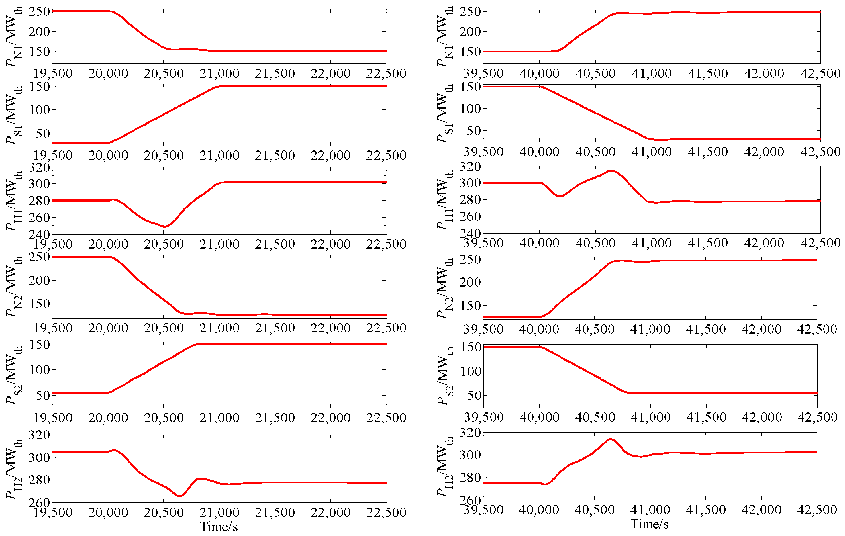
The responses of 1# MHTGR-based OTSSS, i.e., the normalized nuclear power, reactor outlet helium temperature, live steam temperature, primary helium flowrate and secondary feedwater flowrate are shown in Figure 10 and the responses of 2# MHTGR-based OTSSS are shown in Figure 11. The responses of 1# SPT-based OTSSS, i.e., the outlet and inlet molten salt of the receiver, live steam temperature, flowrates of molten salt and feedwater are shown in Figure 12 and the responses of 2# SPT-based OTSSS are given in Figure 13. The responses of main steam pressure, header given by 1# and 2# feedwater pump and fluid resistance caused by governing valves in branch 3 and 4 are all given in Figure 14. The responses thermal power of different OTSSSs and HES modules are shown in Figure 15.
4.3.3. Discussions
The transience happens at 20,000 s is just a switch from nuclear power to solar power. From the left column of Figure 10, Figure 11 and Figure 15, it can be seen that 1# and 2# MHTGR-based OTSSSs maneuver stably from the power-level of 250 MWth to that of 150 and 125 MWth respectively. From the left column of Figure 12, Figure 13 and Figure 15, it can also be seen that the power-levels of 1# and 2# STP-based OTSSS increase smoothly from 30 and 50 to 150 MWth respectively. This power-level maneuver of different OTSSSs relies not only on the control laws of MHTGR-based and STP-based OTSSSs but also heavily on the pressure-flowrate control of secondary FFN with topological structure shown in Figure 9. Since the pump headers is utilized to control the feedwater flowrates of the MHTGR-based OTSSSs, the headers should be reduced in the case of MHTGR power-level decrease. However, the power increase of STP-based OTSSSs needs the increase of feedwater header, which is in contradict with the reduction of pump headers but can be realized by enlarging the opening of the governing valves located in branch 3 and 4. The variation of the OTSSS flowrates can further induce the fluctuation of main steam pressure, which can be suppressed by the steam valve mounted in branch 5. From the left column of Figure 14, FFN control law (57) can guarantee satisfactory transience for branch flowrates and stability for main steam pressure.
Similarly, the transience starts at 40,000 s is a switch from solar power to nuclear power, which may be happens in cloudy days or nighttime. The MHTGR power-level increase needs the increase in pump headers that are adopted to regulate the feedwater flowrates of MHTGR-based OTSSSs, which can also lead to the increase of the feedwater flowrates of STP-based OTSSSs. To realize decrease the feedwater flowrates of STP-based OTSSSs, which is necessary for power-level reduction, the opening of the governing valves in branches 3 and 4 should be lessen. The steam pressure should also be well maintained during the switch from solar power to nuclear power. As we can see from the right column of Figure 14, due to the feedback effect of FFN controller (57), the responses of branch flowrates and steam pressures are satisfactory. Moreover, from the right column of Figure 10, Figure 11, Figure 12 and Figure 13 and Figure 15, 1# and 2# MHTGR-based OTSSSs maneuver stably from 150 and 125 MWth back to 250 MWth respectively and the thermal powers 1# and 2# STP-based OTSSSs also smoothly decrease to 30 and 50 MWth from 150 MWth.
In a summary, the FFN control law (57) realizes the coordinated control of the two HES modules, constituted by a STP-based OTSSS and an MHTGR-based OTSSS, which plays a key role in building thermally coupled multimoduar and hybrid energy systems. From (57), this newly-built FFN controller is just composed of some simple decentralized PI feedback laws with knowledge of plant physical and thermal-hydraulic parameters which are easy to be implemented and commissioned on current digital control system platforms.
5. Conclusions
Multimodular and hybrid energy systems can be built by integrating multiple homogeneous or heterogeneous OTHSS modules based on renewable, nuclear or fossil energy sources, where the module integration can be realized through FFNs. Thus, modeling and flowrate-pressure control of FFNs is crucial for those multimodular and hybrid energy systems with modules interconnected by FFNs. In the aspect of dynamical modeling, a simple control-design-oriented nonlinear differential-algebraic model for the FFNs with multiple pump branches is first proposed based on branch dynamics and network graph property. In the aspect of control design, a novel adaptive decentralized flowrate-pressure control law is given for FNNs with multiple pumps, which can provide satisfactory closed-loop stability as well as transient performance and does not need the values of plant physical and thermal-hydraulic parameters. Moreover, this newly-built FFN controller takes a proportional-integral (PI) form with saturation in the integration term, which induces easy practical implementation. Finally, this new controller has been applied to the power-level maneuver of a two-modular nuclear-solar HES constituted by MHTGR-based and STP-based OTSSSs and realize the regulation of feedwater flowrates of different OTSSSs and stabilization of main steam pressure. Simulation results show the feasibility and high performance of this new FFN controller. The novelty of this paper focuses on converting the control of hybrid and multimodular energy system to modeling and flowrate-pressure control design for FFNs. One of the future research work is to apply the results in this paper to the control of other types of HESs driven by the fossil, nuclear and renewables.
Acknowledgments
This work is jointly supported by the National S&T Major Project of China (Grant Nos. 2008ZX06901, 2010ZX06906) and the Natural Science Foundation of China (NSFC) (Grant No. 61374045, 61773228).
Author Contributions
Zhe Dong gave the modeling and the pressure-fowrate control law for fluid flow networks. Yifei Pan developed the simulation software, and did the verification. Zuoyi Zhang, Yujie Dong and Xiaojin Huang led this research work. Zuoyi Zhang provides the design result of the MHTGR-based NSSS. Yujie Dong gives the design result for the secondary-circuit of the plant. Xiaojin Huang develops the operation strategy for the hybrid plant.
Conflicts of Interest
The authors declare no conflict of interest.
References
- Ruth, M.F.; Zinaman, O.R.; Antkowiak, M.; Boardman, R.D.; Cherry, R.S.; Bazilian, M.D. Nuclear-renewable hybrid energy systems: Opportunities, interconnections and needs. Energy Convers. Manag. 2014, 78, 684–694. [Google Scholar] [CrossRef]
- Montes, M.J.; Rovira, A.; Muñoz, M.; Martínez-Val, J.M. Performance analysis of an integrated solar combined cycle using direct steam generation in parabolic through collectors. Appl. Energy 2011, 88, 3228–3238. [Google Scholar] [CrossRef]
- Ingersoll, D.T. Deliberately small reactors and the second nuclear era. Prog. Nucl. Energy 2009, 51, 589–603. [Google Scholar] [CrossRef]
- Vujić, J.; Bergmann, R.M.; Škoda, R.; Miletić, M. Small modular reactors: Simpler, safer, cheaper? Energy 2012, 45, 288–295. [Google Scholar] [CrossRef]
- Rowinski, M.K.; White, T.J.; Zhao, J. Small and medium sized reactors (SMR): A review of technology. Renew. Sustain. Energy Rev. 2015, 44, 643–656. [Google Scholar] [CrossRef]
- Ingersoll, D.T.; Houghton, Z.J.; Bromm, R.; Desportes, C. Nuscale small modular reactor for co-generation of electricity and water. Desalination 2014, 340, 84–93. [Google Scholar] [CrossRef]
- Reutler, H.; Lohnert, G.H. The modular high-temperature reactor. Nucl. Technol. 1983, 62, 22–30. [Google Scholar] [CrossRef]
- Reutler, H.; Lohnert, G.H. Advantages of going modular. Nucl. Eng. Des. 1984, 78, 129–136. [Google Scholar] [CrossRef]
- Lohnert, G.H. Technical design features and essential safety-related properties of the HTR-MODULE. Nucl. Eng. Des. 1990, 121, 259–275. [Google Scholar] [CrossRef]
- Lanning, D.D. Modularized high-temperature gas-cooled reactor systems. Nucl. Technol. 1989, 88, 139–156. [Google Scholar] [CrossRef]
- Zhang, Z.; Sun, Y. Economic potential of modular reactor nuclear power plants based on the Chinese HTR-PM project. Nucl. Eng. Des. 2007, 237, 2265–2274. [Google Scholar] [CrossRef]
- Zhang, Z.; Wu, Z.; Wang, D.; Xu, Y.; Sun, Y.; Li, F.; Dong, Y. Current status and technical description of Chinese 2 × 250 MWth HTR-PM demonstration plant. Nucl. Eng. Des. 2009, 239, 1212–1219. [Google Scholar] [CrossRef]
- Zhang, Z.; Dong, Y.; Li, F.; Zhang, Z.; Wang, H.; Huang, X.; Li, H.; Liu, B.; Wu, X.; Wang, H.; et al. The shandong shidao bay 200 MWe high-temperature-gas-cooled reactor pebble-bed module (HTR-PM) demonstration power plant: An engineering and technological innovation. Engineering 2016, 2, 112–118. [Google Scholar] [CrossRef]
- Flueckiger, S.M.; Iverson, B.D.; Garimella, S.V.; Pacheco, J.E. System-level simulation of a solar power tower plant with thermocline thermal energy storage. Appl. Energy 2014, 113, 86–96. [Google Scholar] [CrossRef]
- Peng, S.; Hong, H.; Wang, Y.; Wang, Z.; Jin, H. Off-design thermodynamic performances on typical days of a 330MW solar aided coal-fired power plant in China. Appl. Energy 2014, 130, 500–509. [Google Scholar] [CrossRef]
- Kim, K.K.; Bernard, J.A. Considerations in the control of PWR-type multimodular reactor plants. IEEE Trans. Nucl. Sci. 1994, 41, 2686–2697. [Google Scholar]
- Garcia, H.E.; Chen, J.; Kim, J.S.; Vilim, R.B.; Binder, W.R.; Sitton, S.M.B.; Boardman, R.D.; McKellar, M.G.; Paredis, C.J.J. Dynamic performance analysis of two regional nuclear hybrid energy systems. Energy 2016, 107, 234–258. [Google Scholar] [CrossRef]
- Lykidi, M.; Gourdel, P. How to manage flexible nuclear power plants in a deregulated electricity market from the point of view of social welfare? Energy 2015, 85, 167–180. [Google Scholar] [CrossRef]
- Perillo, S.R.P.; Upadhyaya, B.R.; Li, F. Control and instrumentation strategies for multi-modular integral nuclear reactor systems. IEEE Trans. Nucl. Sci. 2011, 58, 2442–2451. [Google Scholar] [CrossRef]
- Dong, Z.; Song, M.; Huang, X.; Zhang, Z.; Wu, Z. Module coordination control of MHTGR-based multi-modular nuclear plants. IEEE Trans. Nucl. Sci. 2016, 63, 1889–1900. [Google Scholar] [CrossRef]
- Zhang, H.L.; Baeyens, J.; Degrѐve, J.; Cacѐres, G. Concentrated solar power plants: Review and design methodology. Renew. Sustain. Energy Rev. 2013, 22, 466–481. [Google Scholar] [CrossRef]
- Mahdi, A.A.; McPherson, M.J. An introduction to automatic control of mine ventilation systems. Min. Technol. 1971, 53, 5–10. [Google Scholar]
- DeMoyer, R.J. System modeling and simulation for water distribution control. Model. Simul. 1974, 5, 185. [Google Scholar]
- Rao, H.S. Modeling of water distribution systems. In Proceedings of the 16th IEEE Conference on Decision and Control, New York, NY, USA, 7–9 December 1977; pp. 653–658. [Google Scholar]
- Kocić, D.D. On the autonomy of local systems in ventilation control. In Proceedings of the 2nd Mine Ventilation Congress, Reno, NV, USA, 4–8 November 1979. [Google Scholar]
- Hu, Y.; Koroleva, O.I.; Kristić, M. Nonlinear control of mine ventilation networks. Syst. Control Lett. 2003, 49, 239–254. [Google Scholar] [CrossRef]
- Dong, Z. Dissipation analysis and adaptive control of fluid networks. In Proceedings of the American Control Conference, Chicago, IL, USA, 1–3 July 2015; pp. 671–676. [Google Scholar]
- Dong, Z.; Song, M.; Huang, X.; Zhang, Z.; Wu, Z. Coordination control of SMR-based NSSS modules integrated by feedwater distribution. IEEE Trans. Nucl. Sci. 2016, 63, 2682–2690. [Google Scholar] [CrossRef]
- Ward-Smith, A.J. Internal Fluid Flow—The Fluid Dynamics of Flow in Pipes and Ducts; Clarendon Press: Oxford, UK, 1980. [Google Scholar]
- Desoer, C.A.; Kuh, E.S. Basic Circuit Theory; McGraw-Hill: New York, NY, USA, 1969. [Google Scholar]
- Reddy, V.S.; Kaushik, S.C.; Ranjan, K.R.; Tyagi, S.K. State-of-the-art of solar thermal power plants—A review. Renew. Sustain. Energy Rev. 2013, 27, 258–273. [Google Scholar] [CrossRef]
- Li, X.; Kong, W.; Wang, Z.; Chang, C.; Bai, F. Thermal model and thermodynamic performance of molten salt cavity receiver. Renew. Energy 2010, 35, 981–988. [Google Scholar] [CrossRef]
- Benammar, S.; Khellaf, A.; Mohammedi, K. Contribution to the modeling and simulation of solar power tower plants using energy analysis. Energy Convers. Manag. 2014, 78, 923–930. [Google Scholar] [CrossRef]
- Dong, Z.; Pan, Y.; Zhang, Z.; Dong, Y.; Huang, X. Model-free adaptive control law for nuclear superheated-steam supply systems. Energy 2017, 135, 53–67. [Google Scholar] [CrossRef]
- Camacho, E.F.; Rubio, F.R.; Berenguel, M.; Valenzuela, L. A survey on control schemes for distributed solar collector fields. Part I: Modeling and basic control approaches. Sol. Energy 2007, 81, 1240–1251. [Google Scholar] [CrossRef]
- Cirre, C.M.; Berenguel, M.; Valenzuela, L.; Camacho, E.F. Feedback linearization control for a distributed solar collector field. Control Eng. Pract. 2007, 15, 1533–1544. [Google Scholar] [CrossRef]
Figure 1.
Schematic diagram of a once-through heat supply system (OTHSS) module.
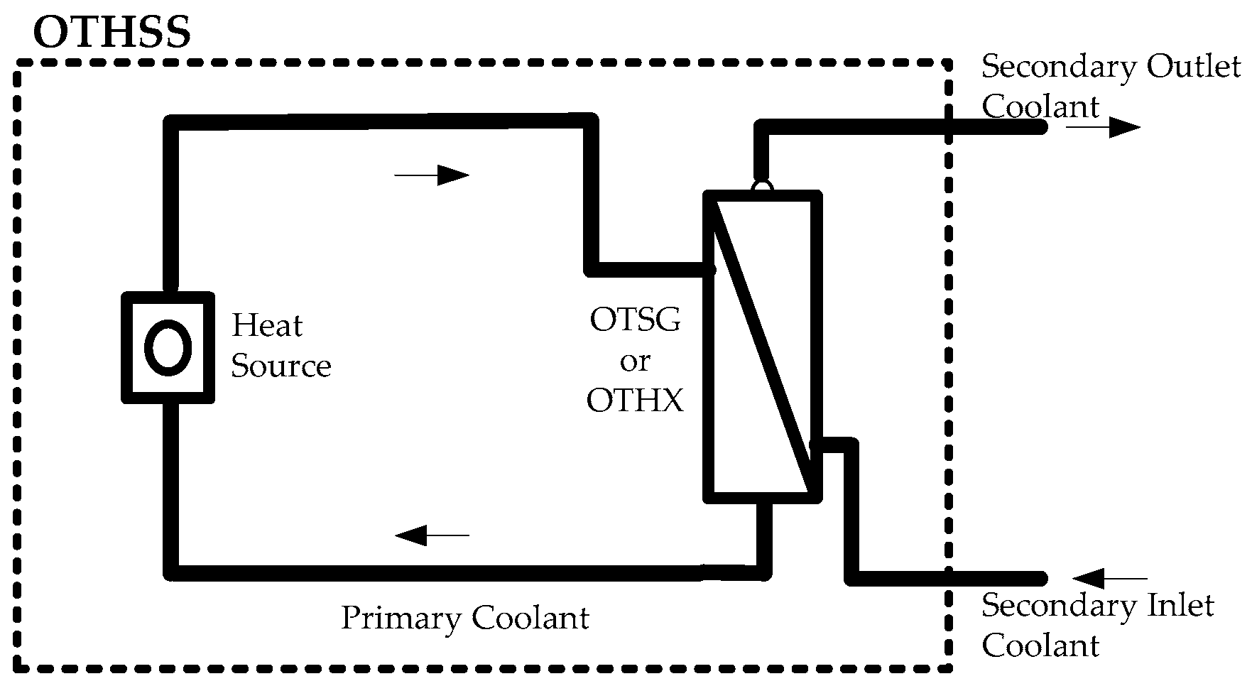
Figure 2.
Schematic diagram of a two-modular international reactor innovative and secure (IRIS)-based plant.
Figure 2.
Schematic diagram of a two-modular international reactor innovative and secure (IRIS)-based plant.

Figure 3.
Secondary-side fluid flow network (FFN) of (a) 2 and (b) m modular IRIS plant by feedwater distribution.
Figure 3.
Secondary-side fluid flow network (FFN) of (a) 2 and (b) m modular IRIS plant by feedwater distribution.
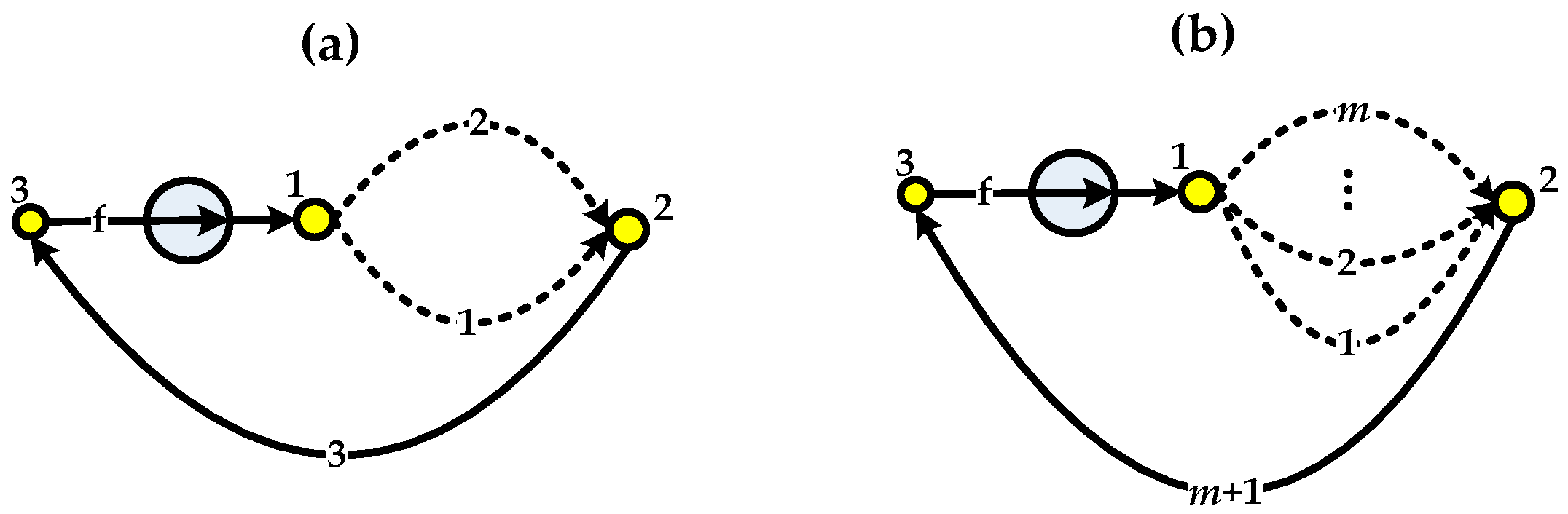
Figure 4.
Schematic diagram of the high temperature reactor (HTR)-PM plant.
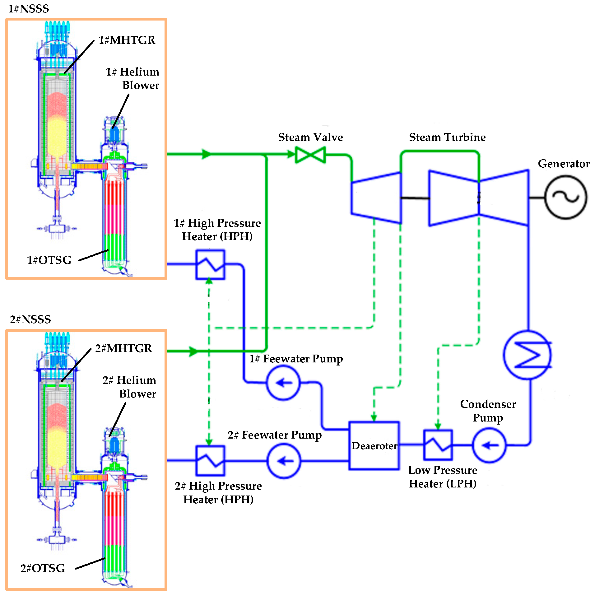
Figure 5.
Secondary-side FFN of (a) 2 and (b) m modular high temperature gas-cooled reactor (MHTGR) plant by independent feedwater strategy.
Figure 5.
Secondary-side FFN of (a) 2 and (b) m modular high temperature gas-cooled reactor (MHTGR) plant by independent feedwater strategy.
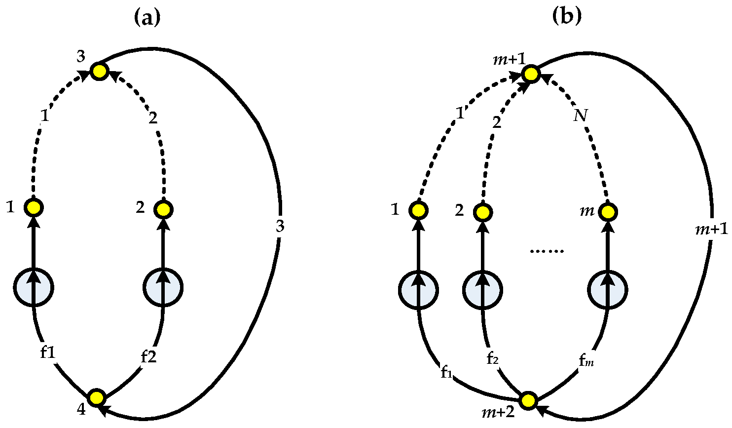
Figure 6.
A nuclear-solar hybrid energy system (HES) constituted by an MHTGR-based and a solar power tower STP-based OTSSSs.
Figure 6.
A nuclear-solar hybrid energy system (HES) constituted by an MHTGR-based and a solar power tower STP-based OTSSSs.
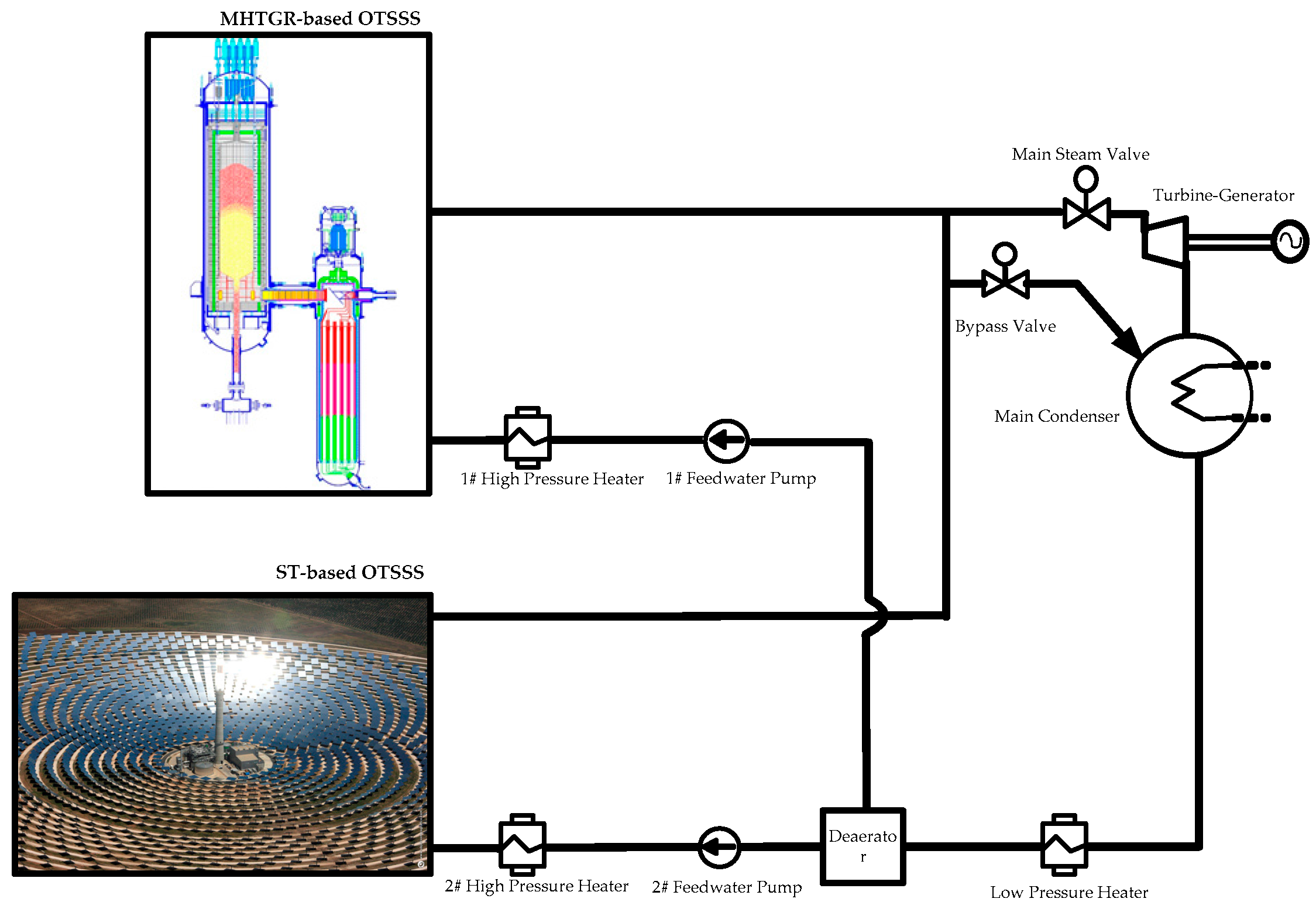
Figure 7.
An HES constituted by an MHTGR-based OTSSS module and a parabolic through collector (PTC)-based OTHSS module: (a) simplified process diagram; (b) structure of the FFN.
Figure 7.
An HES constituted by an MHTGR-based OTSSS module and a parabolic through collector (PTC)-based OTHSS module: (a) simplified process diagram; (b) structure of the FFN.

Figure 8.
Schematic diagram of a nuclear-solar multimodular hybrid energy system (HES).

Figure 9.
FFN of the nuclear-solar hybrid energy system (HES).
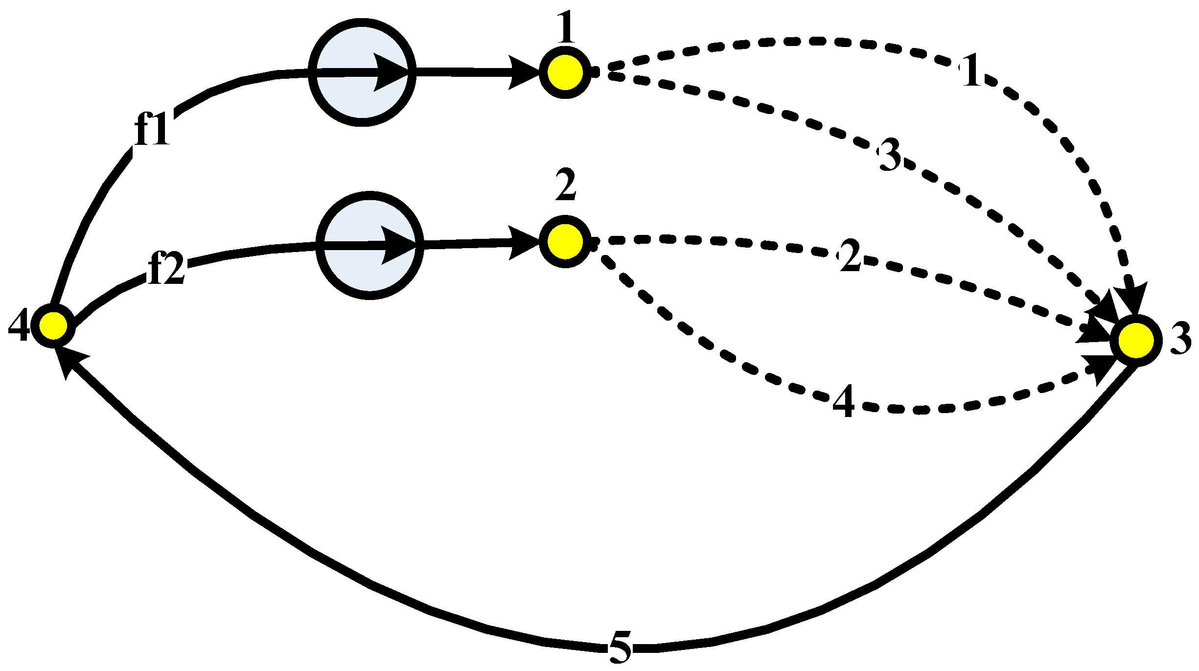
Figure 10.
Responses of 1# MHTGR-based OTSSS, nr1: normalized nuclear power, Tcout1: reactor outlet helium temperature, Ts1: live steam temperature, Gh1: primary helium flowrate, Gfw1: secondary feedwater flowrate.
Figure 10.
Responses of 1# MHTGR-based OTSSS, nr1: normalized nuclear power, Tcout1: reactor outlet helium temperature, Ts1: live steam temperature, Gh1: primary helium flowrate, Gfw1: secondary feedwater flowrate.
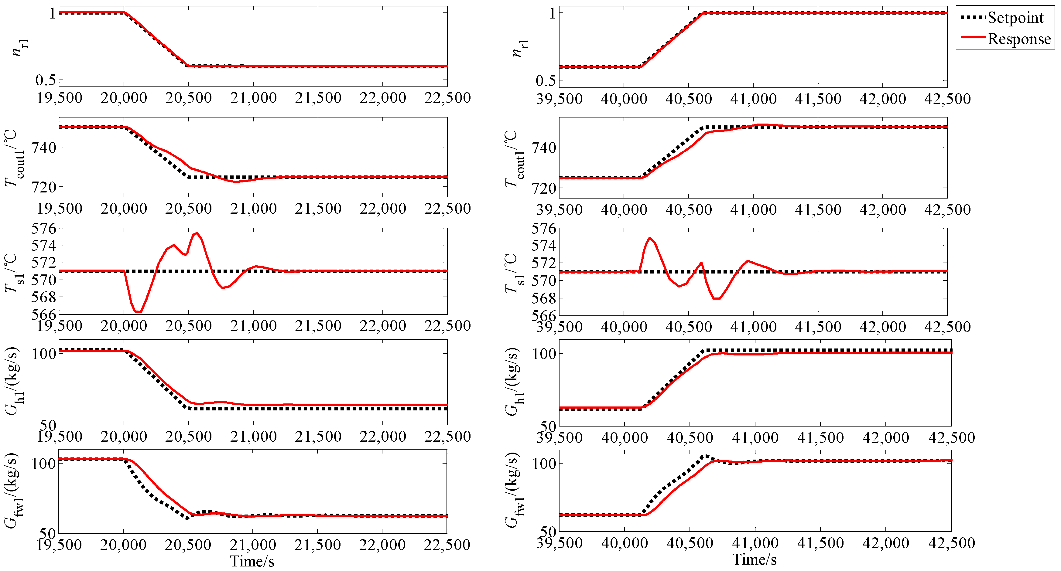
Figure 11.
Responses of 2# MHTGR-based OTSSS, nr2: normalized nuclear power, Tcout2: reactor outlet helium temperature, Tst2: live steam temperature, Gh2: primary helium flowrate, Gfw2: secondary feedwater flowrate.
Figure 11.
Responses of 2# MHTGR-based OTSSS, nr2: normalized nuclear power, Tcout2: reactor outlet helium temperature, Tst2: live steam temperature, Gh2: primary helium flowrate, Gfw2: secondary feedwater flowrate.
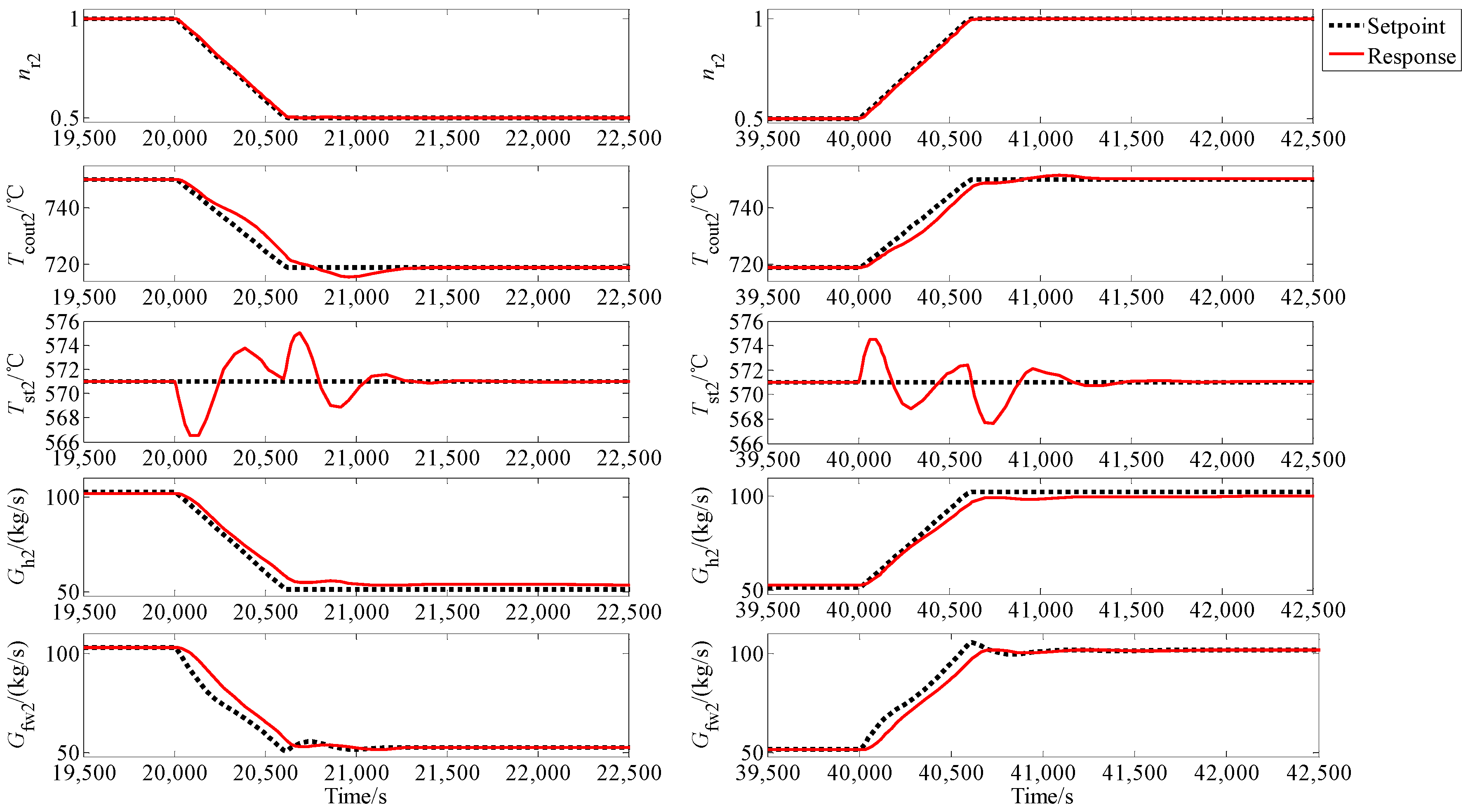
Figure 12.
Responses of 1# STP-based OTSSS, Tmso3: receiver outlet molten salt temperature, Tmsi3: receiver inlet molten salt temperature, Tst3: live steam temperature, Gms1: primary molton salt flowrate, Gfw1: secondary feedwater flowrate.
Figure 12.
Responses of 1# STP-based OTSSS, Tmso3: receiver outlet molten salt temperature, Tmsi3: receiver inlet molten salt temperature, Tst3: live steam temperature, Gms1: primary molton salt flowrate, Gfw1: secondary feedwater flowrate.
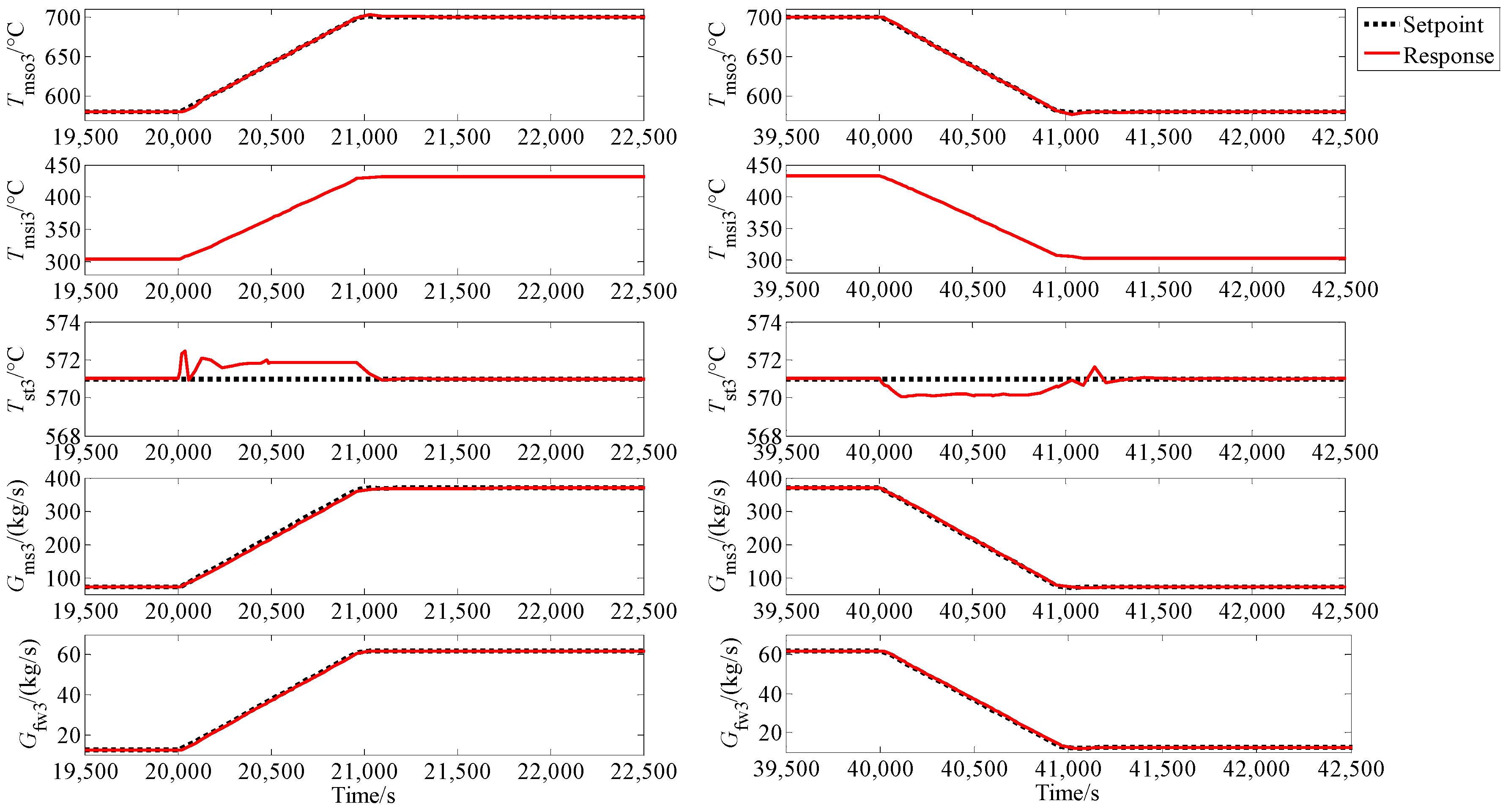
Figure 13.
Responses of 2# STP-based OTSSS, Tmso4: receiver outlet molten salt temperature, Tmsi4: receiver inlet molten salt temperature, Tst4: live steam temperature, Gms4: primary molton salt flowrate, Gfw4: secondary feedwater flowrate.
Figure 13.
Responses of 2# STP-based OTSSS, Tmso4: receiver outlet molten salt temperature, Tmsi4: receiver inlet molten salt temperature, Tst4: live steam temperature, Gms4: primary molton salt flowrate, Gfw4: secondary feedwater flowrate.
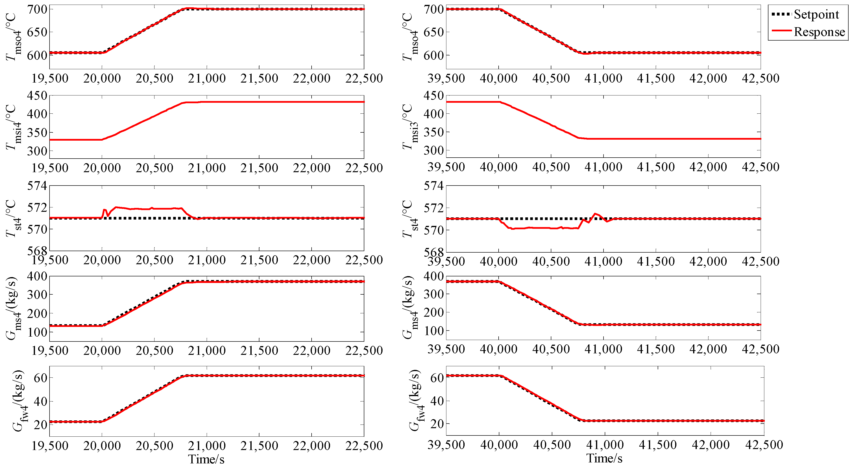
Figure 14.
Responses of main steam pressure, feedwater header and branch resistances, Pst: main steam pressure, Hf1 and Hf2: header given by 1# and 2# feedwater pump, Ri: fluid resistances in branch i (i = 3, 4, 5).
Figure 14.
Responses of main steam pressure, feedwater header and branch resistances, Pst: main steam pressure, Hf1 and Hf2: header given by 1# and 2# feedwater pump, Ri: fluid resistances in branch i (i = 3, 4, 5).
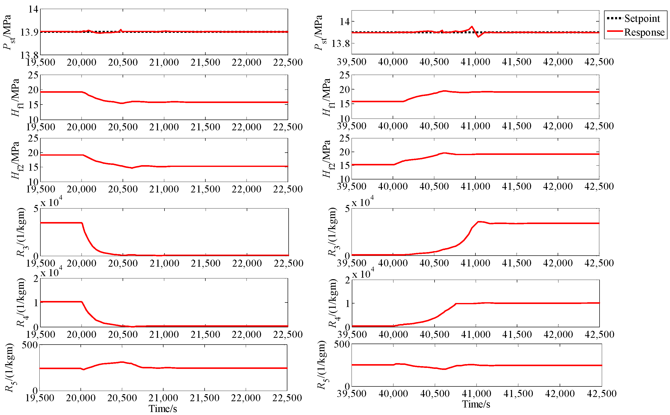
Figure 15.
Responses of thermal powers, PNi: thermal power of i# MHTGR-based OTSSS, PSi: thermal power of i# STP-based OTSSS, PHi thermal power of i# HES module composed of i# MHTGR-based OTSSS and i# STP-based OTSSS (i = 1, 2).
Figure 15.
Responses of thermal powers, PNi: thermal power of i# MHTGR-based OTSSS, PSi: thermal power of i# STP-based OTSSS, PHi thermal power of i# HES module composed of i# MHTGR-based OTSSS and i# STP-based OTSSS (i = 1, 2).

Table 1.
Main design parameters of the nuclear-solar hybrid energy system (HES) at rated condition.
| Parameter | Unit | Value | |
|---|---|---|---|
| Plant | Maximal Plant thermal power | MWt | 800 |
| Maximal Plant electrical power | MWe | 320 | |
| Number of modules | 2 | ||
| Main steam temperature | °C | 571 | |
| Main steam pressure | MPa | 13.9 | |
| MHTGR-Based OTSSS | Rated thermal power | MWth | 250 |
| Average core power density | MW/m3 | 3.22 | |
| Active core diameter/height | m | 3/11 | |
| Primary helium pressure | MPa | 7 | |
| Helium temperature at reactor inlet/outlet | °C | 277/750 | |
| Helium flowrate | kg/s | 102 | |
| Feedwater temperature | °C | 250 | |
| Feedwater flowrate | kg/s | 103 | |
| STP-Based OTSSS | Rated thermal power | MWth | 150 |
| Heat transfer fluid (HTF) | Molten nitrate salt mixture (60 wt % NaNO3, 40 wt % KNO3) | ||
| HTF temperature at cold/hot leg | °C | 432/700 | |
| HTF flowrate | kg/s | 368 | |
| Feedwater temperature | °C | 250 | |
| Feedwater flowrate | kg/s | 61 |
© 2017 by the authors. Licensee MDPI, Basel, Switzerland. This article is an open access article distributed under the terms and conditions of the Creative Commons Attribution (CC BY) license (http://creativecommons.org/licenses/by/4.0/).
Share and Cite
MDPI and ACS Style
Dong, Z.; Pan, Y.; Zhang, Z.; Dong, Y.; Huang, X. Modeling and Control of Fluid Flow Networks with Application to a Nuclear-Solar Hybrid Plant. Energies 2017, 10, 1912. https://doi.org/10.3390/en10111912
AMA Style
Dong Z, Pan Y, Zhang Z, Dong Y, Huang X. Modeling and Control of Fluid Flow Networks with Application to a Nuclear-Solar Hybrid Plant. Energies. 2017; 10(11):1912. https://doi.org/10.3390/en10111912
Chicago/Turabian StyleDong, Zhe, Yifei Pan, Zuoyi Zhang, Yujie Dong, and Xiaojin Huang. 2017. "Modeling and Control of Fluid Flow Networks with Application to a Nuclear-Solar Hybrid Plant" Energies 10, no. 11: 1912. https://doi.org/10.3390/en10111912
Note that from the first issue of 2016, this journal uses article numbers instead of page numbers. See further details here.