Failure Prognosis of High Voltage Circuit Breakers with Temporal Latent Dirichlet Allocation †


Abstract
:1. Introduction
- (1)
- Weak correlation. The underlying hypothesis behind association-based sequence mining, especially for the rule-based methods, is the strong correlation between events. In contrast, the dependency of the failures on HVCBs is much weaker and probabilistic.
- (2)
- Complexity. The primary objective of most existing applications is a binary decision: whether a failure will happen or not. However, accurate life-cycle management requires information about which failure might occur. The increasing complexity of encoding categories into sequential values can impose serious challenges on the analysis method design, which is called the “curse of cardinality”.
- (3)
- Sparsity. Despite the cardinality problem, the types of failure occurring on an individual basis is relatively small. Some events in a single case may have never been observed before, which makes establishing a statistical significance challenging. The inevitable truncation also aggravates the sparsity problem to a higher degree.
2. Data Preprocessing
2.1. Description of the HVCB Event Logs
2.2. Failure Classification
2.3. Sequence Aligning and Spatial Compression
3. Proposed Method
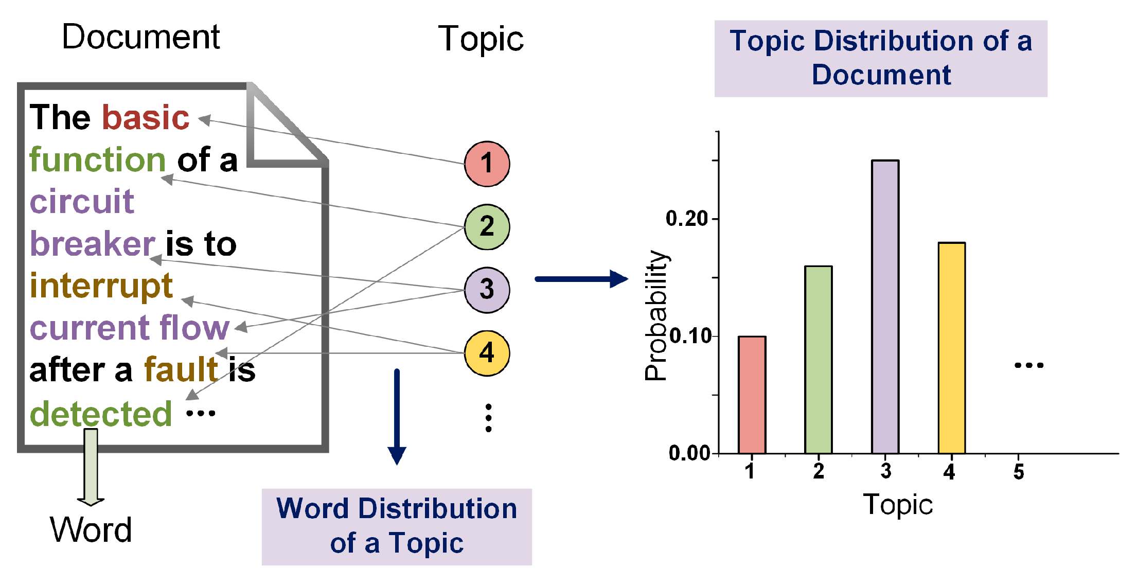
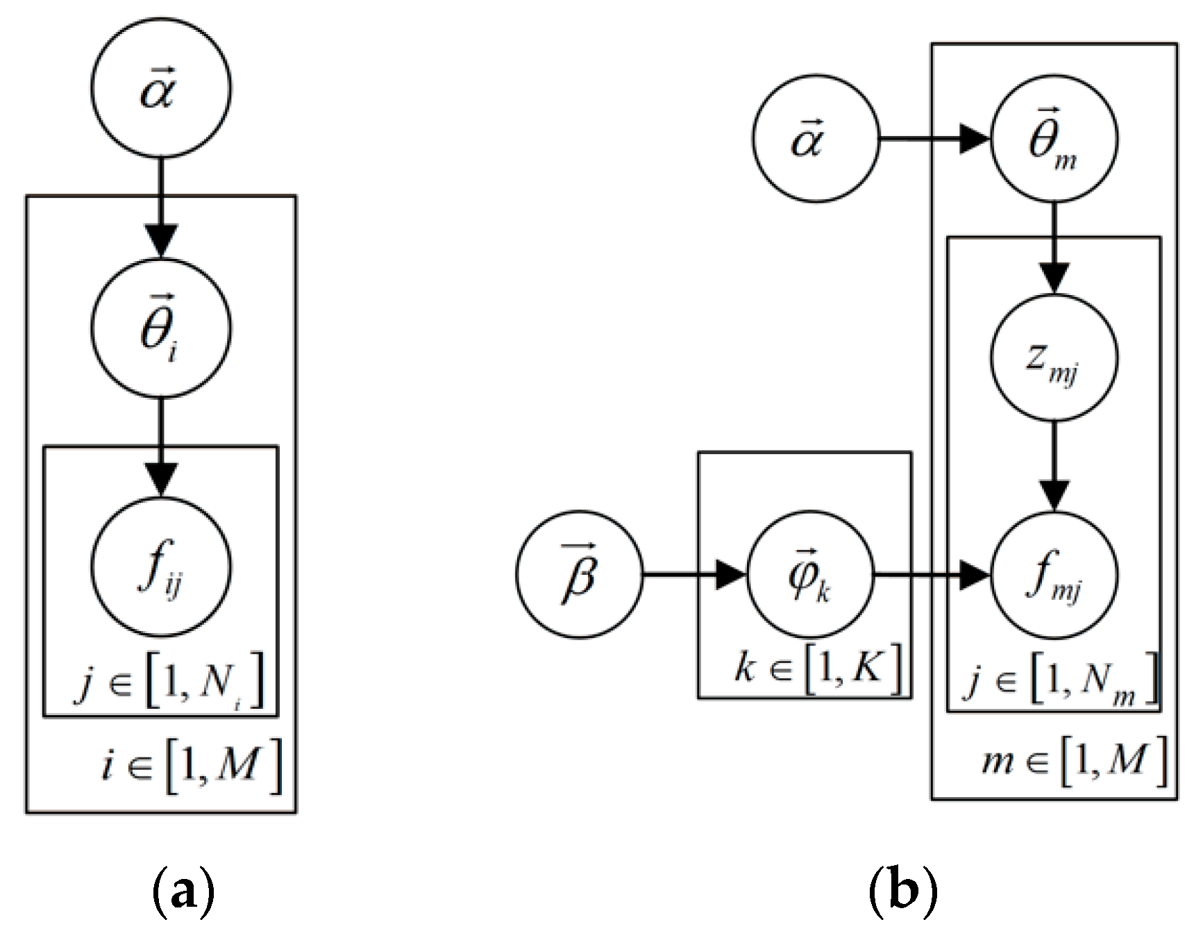
3.1. Latent Dirichlet Allocation Model
3.1.1. Dirichlet Distribution
- (1)
- Choose , where ;
- (2)
- Choose a failure , where .
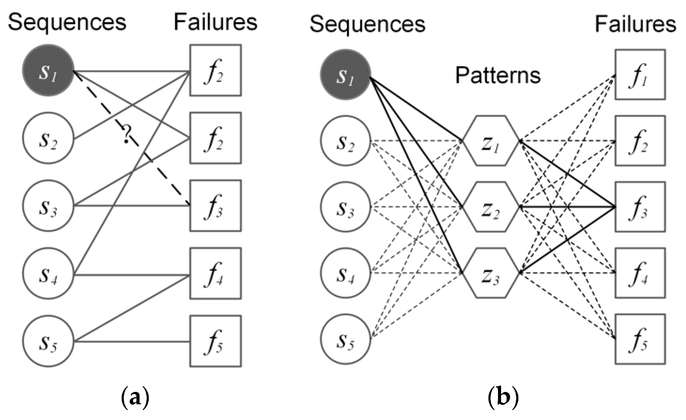
3.1.2. Latent Layer
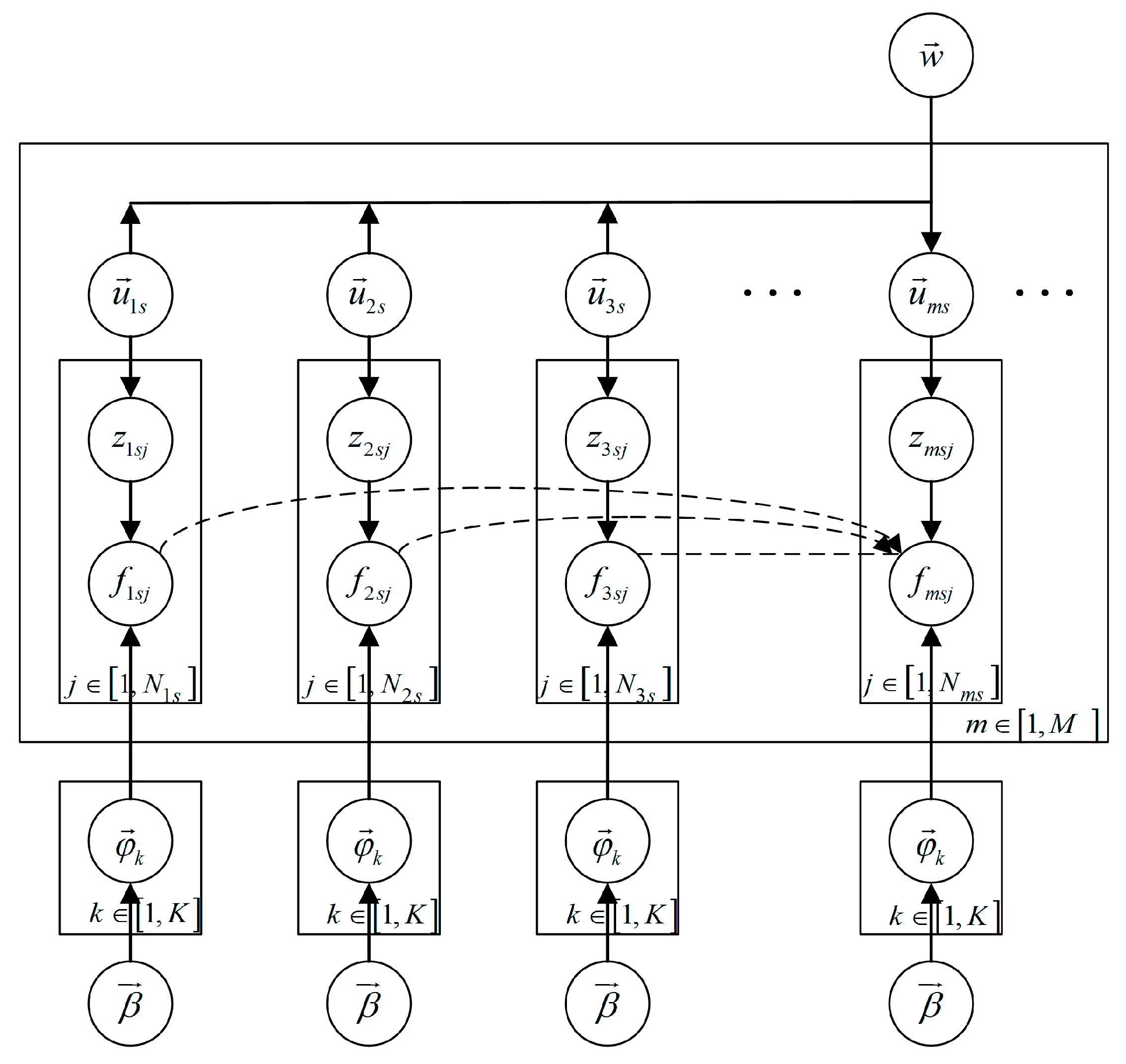
3.1.3. Latent Dirichlet Allocation
- (1)
- Choose , where ;
- (2)
- Choose , where ;For each failure ,
- (3)
- Choose a latent value ;
- (4)
- Choose a failure .
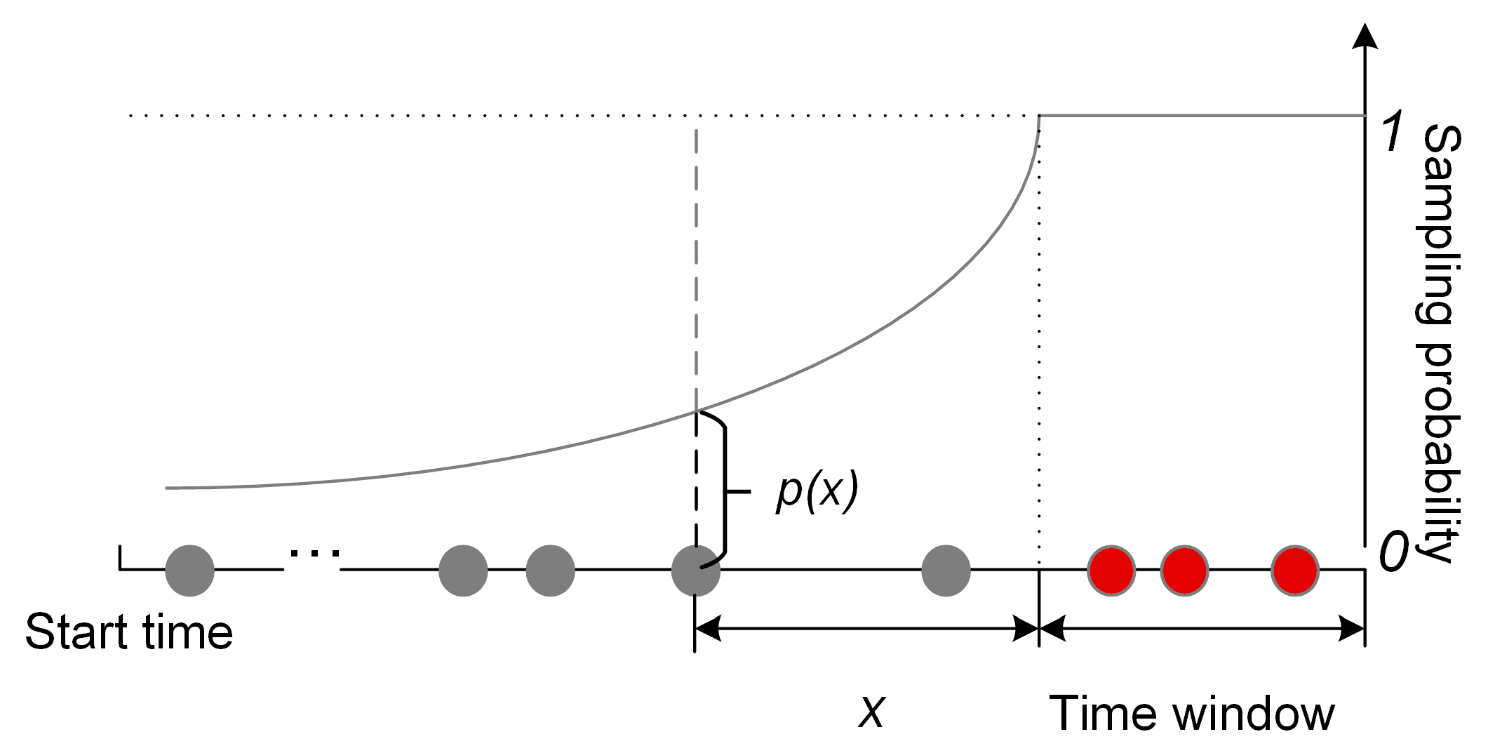
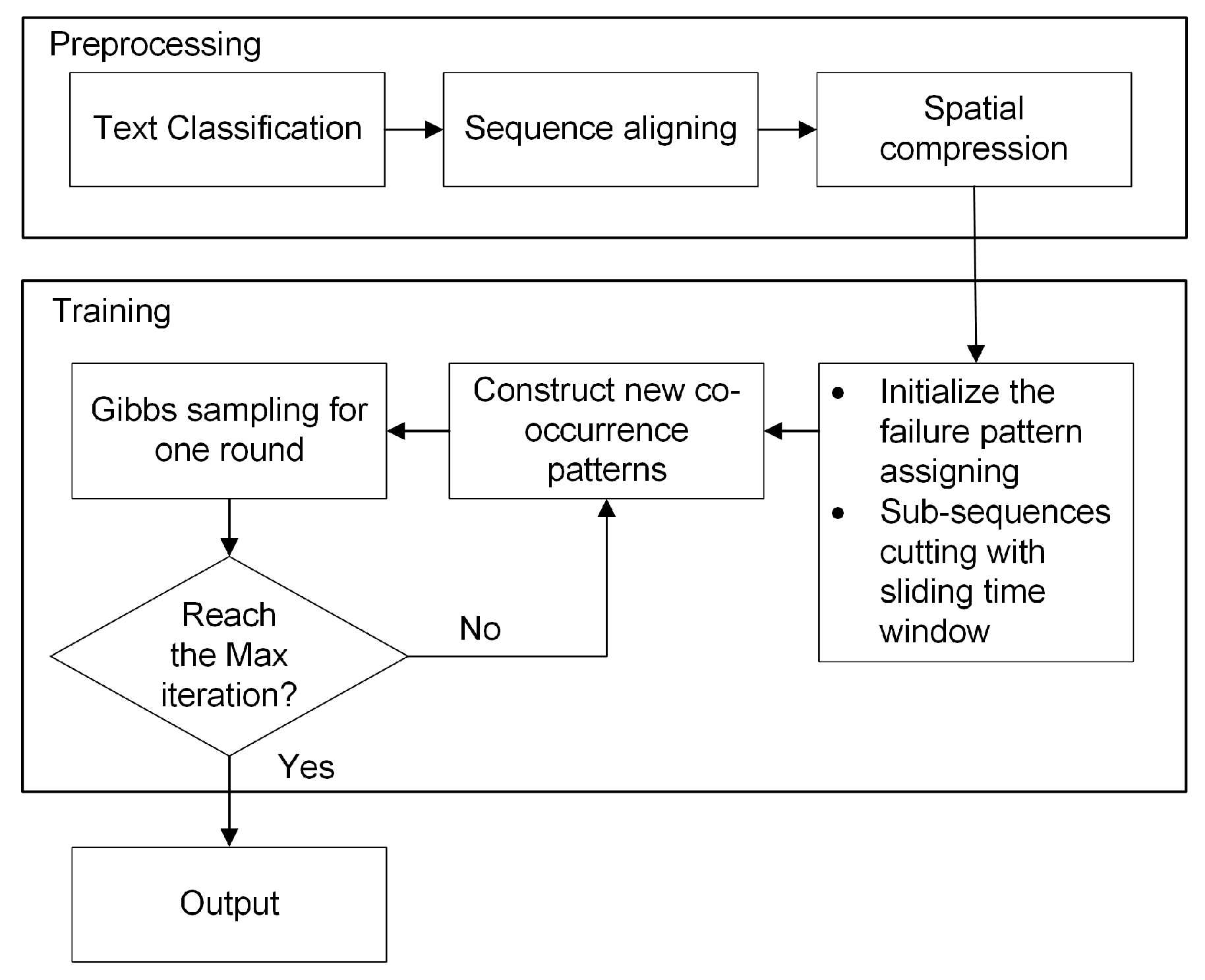
3.2. Introducing the Temporal Association into LDA
| Algorithm 1 Gibbs sampling with the new co-occurrence patterns | |
| Input: Sequences, MaxIteration, , , , | |
| Output: posterior inference of and | |
| 1: | Initialization: randomly assign failure patterns and make sub-sequences by ; |
| 2: | Compute the statistics , , , in Equation (11) for each sub-sequence; |
| 3: | for iter in 1 to MaxIteration do |
| 4: | Foreach sequence in Sequences do |
| 5: | Foreach sub-sequence in sequence do |
| 6: | Add new failures in the current sub-sequence based on Equation (16); |
| 7: | Foreach failure in the new sub-sequence do |
| 8: | Draw new from Equation (11); |
| 9: | Update the statistics in Equation (11); |
| 10: | End for |
| 11: | End for |
| 12: | End for |
| 13: | Compute the posterior mean of and based on Equations (12) and (13) |
| 14: | End for |
| 15: | Compute the mean of and of last several iterations |
4. Evaluation Criteria
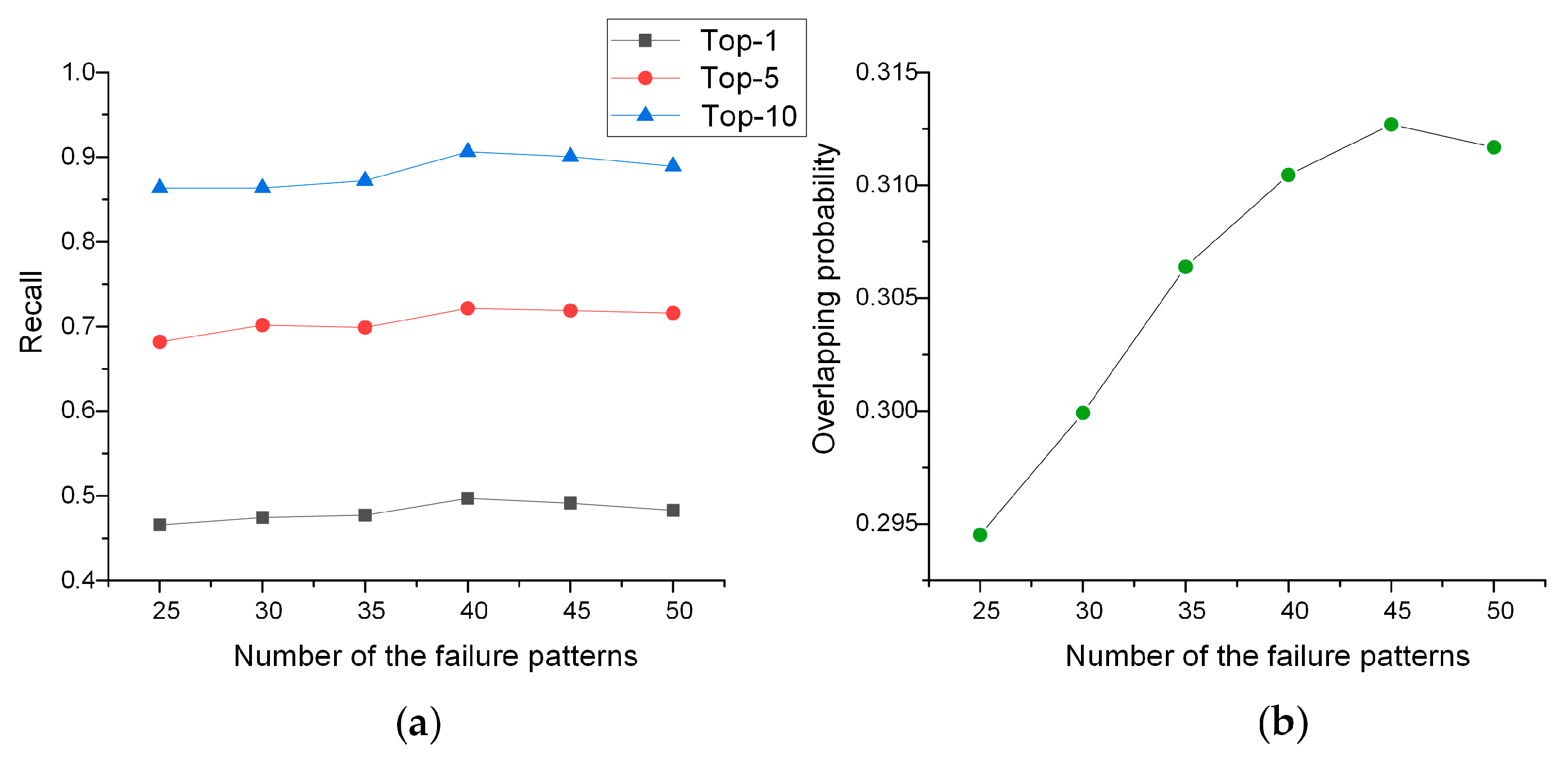
4.1. Quantitative Criteria
4.1.1. Top-N Recall
4.1.2. Overlapping Probability
4.2. Qualitative Criteria
5. Case Study
5.1. Quantitative Analysis
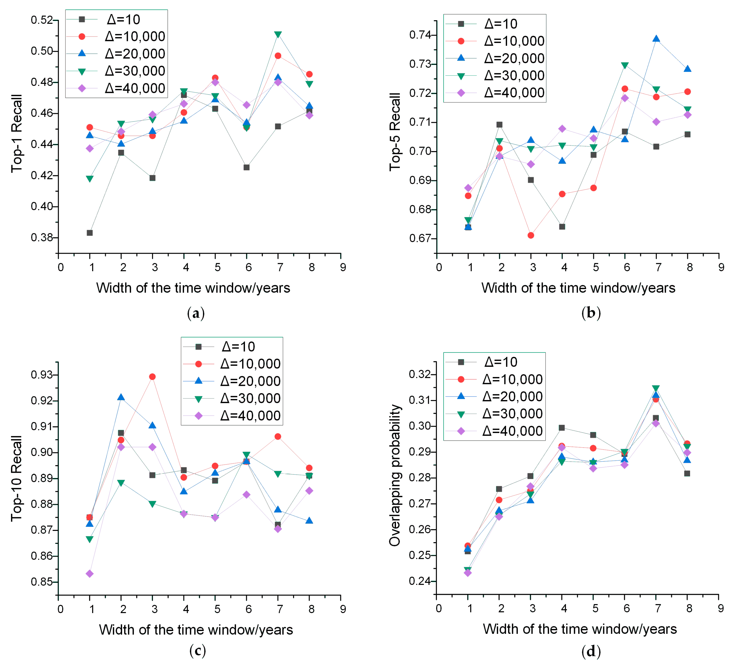
5.1.1. Parameter Analysis
5.1.2. Comparison with Baselines
5.2. Qualitative Analysis
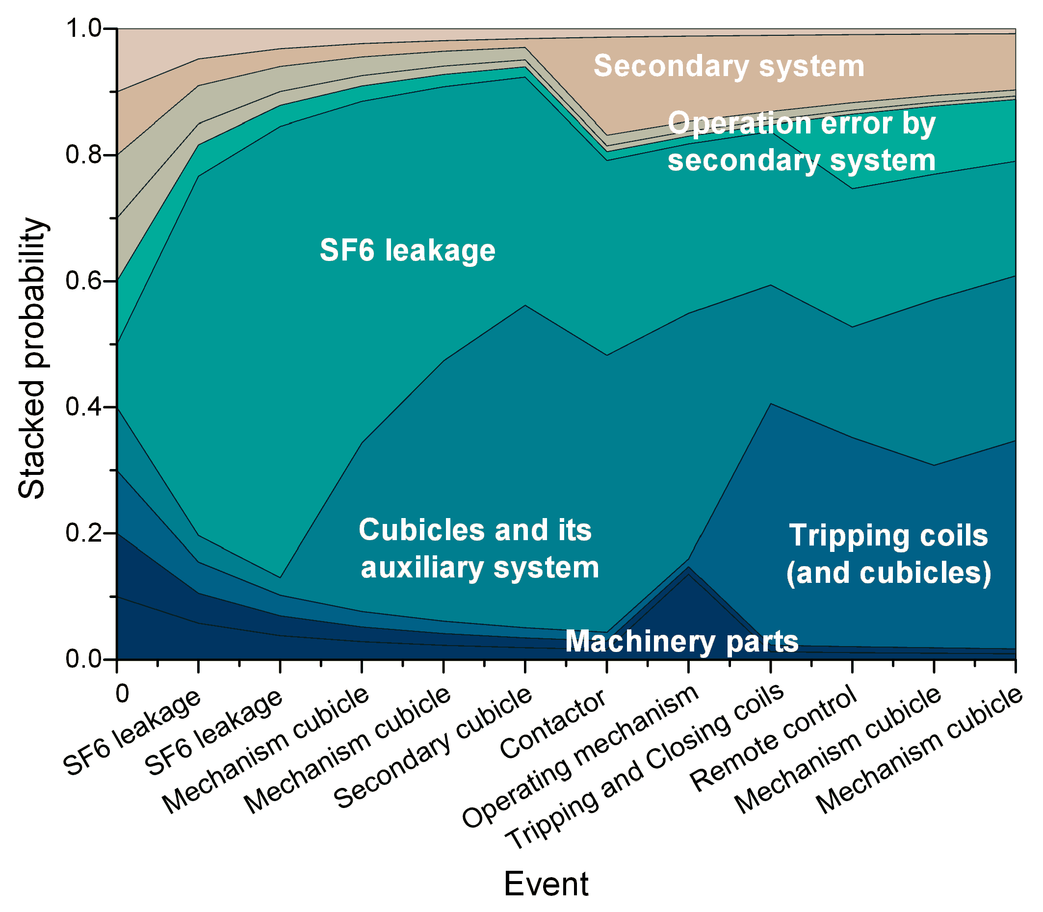
5.2.1. Failure Patterns Extraction
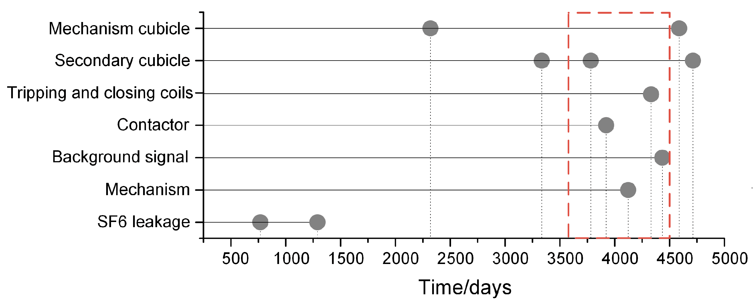
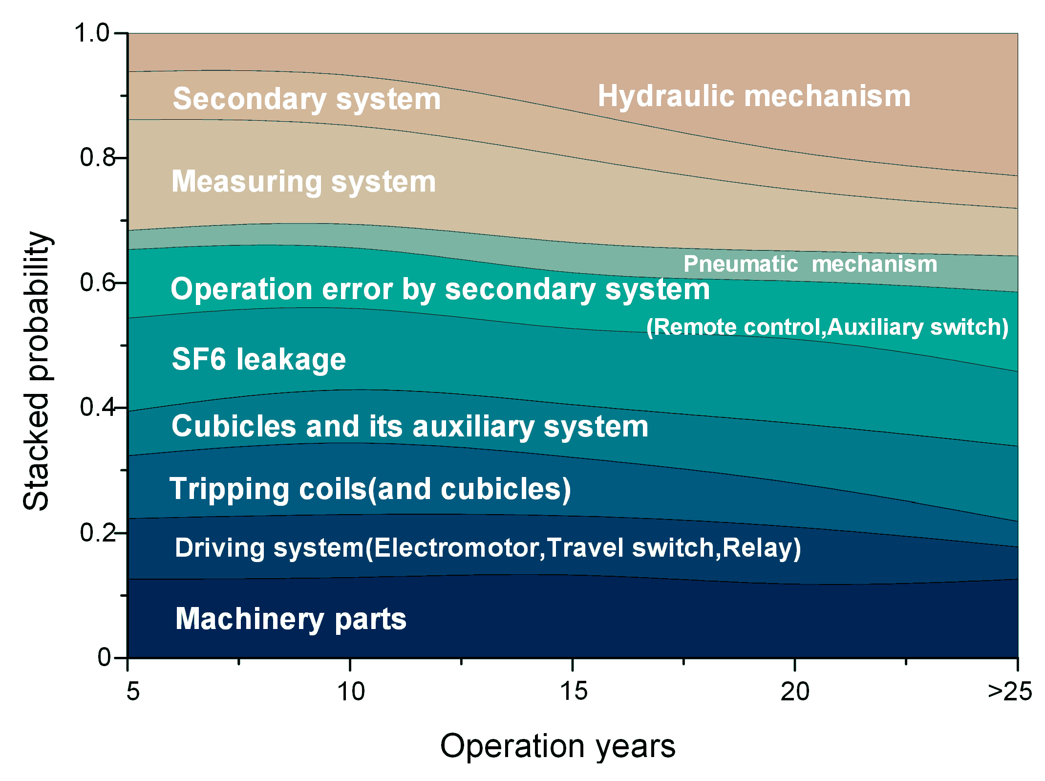
5.2.2. Temporal Features of the Failure Patterns
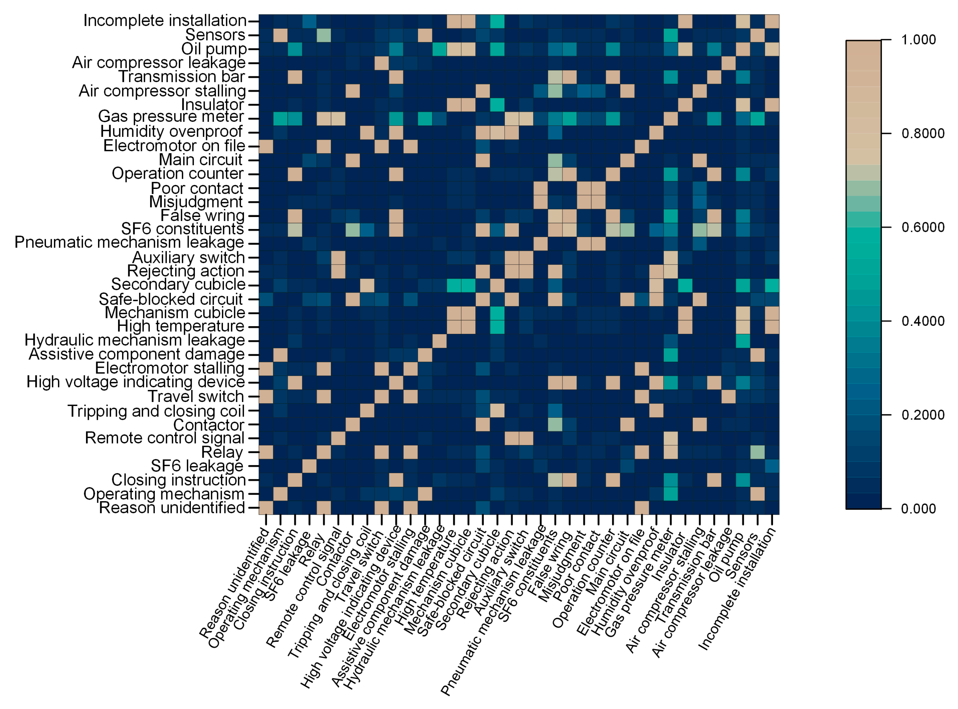
5.2.3. Similarities between Failures
6. Conclusions and Future Work
Acknowledgments
Author Contributions
Conflicts of Interest
References
- Hale, P.S.; Arno, R.G. Survey of reliability and availability information for power distribution, power generation, and HVAC components for commercial, industrial, and utility installations. IEEE Trans. Ind. Appl. 2001, 37, 191–196. [Google Scholar] [CrossRef]
- Lindquist, T.M.; Bertling, L.; Eriksson, R. Circuit breaker failure data and reliability modelling. IET Gener. Transm. Distrib. 2008, 2, 813–820. [Google Scholar] [CrossRef]
- Janssen, A.; Makareinis, D.; Solver, C.E. International Surveys on Circuit-Breaker Reliability Data for Substation and System Studies. IEEE Trans. Power Deliv. 2014, 29, 808–814. [Google Scholar] [CrossRef]
- Pitz, V.; Weber, T. Forecasting of circuit-breaker behaviour in high-voltage electrical power systems: Necessity for future maintenance management. J. Intell. Robot. Syst. 2001, 31, 223–228. [Google Scholar] [CrossRef]
- Jardine, A.K.; Lin, D.; Banjevic, D. A review on machinery diagnostics and prognostics implementing condition-based maintenance. Mech. Syst. Signal Process. 2006, 20, 1483–1510. [Google Scholar] [CrossRef]
- Liu, H.; Wang, Y.; Yang, Y.; Liao, R.; Geng, Y.; Zhou, L. A Failure Probability Calculation Method for Power Equipment Based on Multi-Characteristic Parameters. Energies 2017, 10, 704. [Google Scholar] [CrossRef]
- Peng, Y.; Dong, M.; Zuo, M.J. Current status of machine prognostics in condition-based maintenance: A review. Int. J. Adv. Manuf. Technol. 2010, 50, 297–313. [Google Scholar] [CrossRef]
- Rong, M.; Wang, X.; Yang, W.; Jia, S. Mechanical condition recognition of medium-voltage vacuum circuit breaker based on mechanism dynamic features simulation and ANN. IEEE Trans. Power Deliv. 2005, 20, 1904–1909. [Google Scholar] [CrossRef]
- Rusek, B.; Balzer, G.; Holstein, M.; Claessens, M.S. Timings of high voltage circuit-breaker. Electr. Power Syst. Res. 2008, 78, 2011–2016. [Google Scholar] [CrossRef]
- Natti, S.; Kezunovic, M. Assessing circuit breaker performance using condition-based data and Bayesian approach. Electr. Power Syst. Res. 2011, 81, 1796–1804. [Google Scholar] [CrossRef]
- Cheng, T.; Gao, W.; Liu, W.; Li, R. Evaluation method of contact erosion for high voltage SF6 circuit breakers using dynamic contact resistance measurement. Electr. Power Syst. Res. 2017. [Google Scholar] [CrossRef]
- Tang, J.; Jin, M.; Zeng, F.; Zhou, S.; Zhang, X.; Yang, Y.; Ma, Y. Feature Selection for Partial Discharge Severity Assessment in Gas-Insulated Switchgear Based on Minimum Redundancy and Maximum Relevance. Energies 2017, 10, 1516. [Google Scholar] [CrossRef]
- Gao, W.; Zhao, D.; Ding, D.; Yao, S.; Zhao, Y.; Liu, W. Investigation of frequency characteristics of typical pd and the propagation properties in gis. IEEE Trans. Dielectr. Electr. Insul. 2015, 22, 1654–1662. [Google Scholar] [CrossRef]
- Yang, D.; Tang, J.; Yang, X.; Li, K.; Zeng, F.; Yao, Q.; Miao, Y.; Chen, L. Correlation Characteristics Comparison of SF6 Decomposition versus Gas Pressure under Negative DC Partial Discharge Initiated by Two Typical Defects. Energies 2017, 10, 1085. [Google Scholar] [CrossRef]
- Huang, N.; Fang, L.; Cai, G.; Xu, D.; Chen, H.; Nie, Y. Mechanical Fault Diagnosis of High Voltage Circuit Breakers with Unknown Fault Type Using Hybrid Classifier Based on LMD and Time Segmentation Energy Entropy. Entropy 2016, 18, 322. [Google Scholar] [CrossRef]
- Wang, Z.; Jones, G.R.; Spencer, J.W.; Wang, X.; Rong, M. Spectroscopic On-Line Monitoring of Cu/W Contacts Erosion in HVCBs Using Optical-Fibre Based Sensor and Chromatic Methodology. Sensors 2017, 17, 519. [Google Scholar] [CrossRef] [PubMed]
- Tang, J.; Zhuo, R.; Wang, D.; Wu, J.; Zhang, X. Application of SA-SVM incremental algorithm in GIS PD pattern recognition. J. Electr. Eng. Technol. 2016, 11, 192–199. [Google Scholar] [CrossRef]
- Liao, R.; Zheng, H.; Grzybowski, S.; Yang, L.; Zhang, Y.; Liao, Y. An integrated decision-making model for condition assessment of power transformers using fuzzy approach and evidential reasoning. IEEE Trans. Power Deliv. 2011, 26, 1111–1118. [Google Scholar] [CrossRef]
- Jiang, T.; Li, J.; Zheng, Y.; Sun, C. Improved bagging algorithm for pattern recognition in UHF signals of partial discharges. Energies 2011, 4, 1087–1101. [Google Scholar] [CrossRef]
- Mazza, G.; Michaca, R. The first international enquiry on circuit-breaker failures and defects in service. Electra 1981, 79, 21–91. [Google Scholar]
- International Conference on Large High Voltage Electric Systems; Study Committee 13 (Switching Equipment); Working Group 06 (Reliability of HV circuit breakers). Final Report of the Second International Enquiry on High Voltage Circuit-Breaker Failures and Defects in Service; CIGRE: Paris, France, 1994. [Google Scholar]
- Ejnar, S.C.; Antonio, C.; Manuel, C.; Hiroshi, F.; Wolfgang, G.; Antoni, H.; Dagmar, K.; Johan, K.; Mathias, K.; Dirk, M. Final Report of the 2004–2007 International Enquiry on Reliability of High Voltage Equipment; Part 2—Reliability of High Voltage SFCircuit Breakers. Electra 2012, 16, 49–53. [Google Scholar]
- Boudreau, J.F.; Poirier, S. End-of-life assessment of electric power equipment allowing for non-constant hazard rate—Application to circuit breakers. Int. J. Electr. Power Energy Syst. 2014, 62, 556–561. [Google Scholar] [CrossRef]
- Salfner, F.; Lenk, M.; Malek, M. A survey of online failure prediction methods. ACM Comput. Surv. 2010, 42. [Google Scholar] [CrossRef]
- Fu, X.; Ren, R.; Zhan, J.; Zhou, W.; Jia, Z.; Lu, G. LogMaster: Mining Event Correlations in Logs of Large-Scale Cluster Systems. In Proceedings of the 2012 IEEE 31st Symposium on Reliable Distributed Systems (SRDS), Irvine, CA, USA, 8–11 October 2012; IEEE: Piscataway, NJ, USA, 2012; pp. 71–80. [Google Scholar]
- Gainaru, A.; Cappello, F.; Fullop, J.; Trausan-Matu, S.; Kramer, W. Adaptive event prediction strategy with dynamic time window for large-scale hpc systems. In Proceedings of the Managing Large-Scale Systems via the Analysis of System Logs and the Application of Machine Learning Techniques, Cascais, Portugal, 23–26 October 2011; ACM: New York, NY, USA, 2011; p. 4. [Google Scholar]
- Wang, F.; Lee, N.; Hu, J.; Sun, J.; Ebadollahi, S.; Laine, A.F. A framework for mining signatures from event sequences and its applications in healthcare data. IEEE Trans. Pattern Anal. Mach. Intell. 2013, 35, 272–285. [Google Scholar] [CrossRef] [PubMed]
- Macfadyen, L.P.; Dawson, S. Mining LMS data to develop an “early warning system” for educators: A proof of concept. Comput. Educ. 2010, 54, 588–599. [Google Scholar] [CrossRef]
- Agrawal, R.; Imieliński, T.; Swami, A. Mining association rules between sets of items in large databases. In Proceedings of the 1993 ACM SIGMOD International Conference on Management of Data, Washington, DC, USA, 25–28 May 1993; ACM: New York, NY, USA, 1993; pp. 207–216. [Google Scholar]
- Li, Z.; Zhou, S.; Choubey, S.; Sievenpiper, C. Failure event prediction using the Cox proportional hazard model driven by frequent failure signatures. IIE Trans. 2007, 39, 303–315. [Google Scholar] [CrossRef]
- Fronza, I.; Sillitti, A.; Succi, G.; Terho, M.; Vlasenko, J. Failure prediction based on log files using random indexing and support vector machines. J. Syst. Softw. 2013, 86, 2–11. [Google Scholar] [CrossRef]
- Mikolov, T.; Chen, K.; Corrado, G.; Dean, J. Efficient Estimation of Word Representations in Vector Space. Comput.Sci. 2013; arXiv:1301.3781. [Google Scholar]
- Blei, D.M.; Ng, A.Y.; Jordan, M.I. Latent dirichlet allocation. J. Mach. Learn. Res. 2003, 3, 993–1022. [Google Scholar]
- Guo, C.; Li, G.; Zhang, H.; Ju, X.; Zhang, Y.; Wang, X. Defect distribution prognosis of high voltage circuit breakers with enhanced latent Dirichlet allocation. In Proceedings of the Prognostics and System Health Management Conference (PHM-Harbin), Harbin, China, 9–12 July 2017; IEEE: Piscataway, NJ, USA, 2017; pp. 1–7. [Google Scholar]
- Sutskever, I.; Vinyals, O.; Le, Q.V. Sequence to Sequence Learning with Neural Networks. Adv. Neural Inf. Process. Syst. 2014, 4, 3104–3112. [Google Scholar]
- Anderson, C. The Long Tail: Why the Future of Business Is Selling Less of More; Hachette Books: New York, NY, USA, 2006. [Google Scholar]
- Pinoli, P.; Chicco, D.; Masseroli, M. Latent Dirichlet allocation based on Gibbs sampling for gene function prediction. In Proceedings of the 2014 IEEE Conference on Computational Intelligence in Bioinformatics and Computational Biology, Honolulu, HI, USA, 21–24 May 2014; IEEE: Piscataway, NJ, USA, 2014; pp. 1–8. [Google Scholar]
- Wang, X.; Grimson, E. Spatial Latent Dirichlet Allocation. In Proceedings of the Conference on Neural Information Processing Systems, Vancouver, BC, Canada, 3–6 December 2007; pp. 1577–1584. [Google Scholar]
- Maskeri, G.; Sarkar, S.; Heafield, K. Mining business topics in source code using latent dirichlet allocation. In Proceedings of the India Software Engineering Conference, Hyderabad, India, 9–12 February 2008; pp. 113–120. [Google Scholar]
- Golub, G.H.; Van Loan, C.F. Matrix Computations; Johns Hopkins University Press: Baltimore, MD, USA, 1983; pp. 392–396. [Google Scholar]
- Koren, Y.; Bell, R.; Volinsky, C. Matrix factorization techniques for recommender systems. Computer 2009, 42, 30–37. [Google Scholar] [CrossRef]
- Blei, D.M.; Lafferty, J.D. Dynamic topic models. In Proceedings of the 23rd International Conference on Machine Learning, Pittsburgh, PA, USA, 25–29 June 2006; ACM: New York, NY, USA, 2006; pp. 113–120. [Google Scholar]
- Du, L.; Buntine, W.; Jin, H.; Chen, C. Sequential latent Dirichlet allocation. Knowl. Inf. Syst. 2012, 31, 475–503. [Google Scholar] [CrossRef]
- Herlocker, J.L.; Konstan, J.A.; Terveen, L.G.; Riedl, J.T. Evaluating collaborative filtering recommender systems. ACM Trans. Inf. Syst. 2004, 22, 5–53. [Google Scholar] [CrossRef]
- Wei, X.; Croft, W.B. LDA-based document models for ad-hoc retrieval. In Proceedings of the 29th Annual International ACM SIGIR Conference on Research and Development in Information Retrieval, Seattle, WA, USA, 6–10 August 2006; ACM: New York, NY, USA, 2006; pp. 178–185. [Google Scholar]


| Attribute | Content |
|---|---|
| ID | Numerical order of a failure entry |
| Voltage grade | 110 kV, 220 kV, or 550 kV |
| Substation | Location of the equipment failure, e.g., ShenZhen station |
| Product model | Specified model number, e.g., JWG1-126 |
| Equipment type | A board taxonomy, e.g., high-voltage isolator, gas insulated switchgear (GIS) |
| Failure description | Detailed description of the phenomena observed |
| Failure reason | Cause of the failure |
| Failure time | Time when a failure was recorded |
| Processing measures | Performed operation to repair the high voltage circuit breaker (HVCB) |
| Processing result | Performance report after repair |
| Repair time | Time when a failure was removed |
| Installing time | Time when a HVCB was first put into production |
| Others | Including the person responsible, mechanism type, a rough classification, manufacturers, etc. |
| Failure Description | Failure Reason | Processing Measures |
|---|---|---|
| Circuit breakers connected with the high voltage side of the main transformer cannot close or open. The power supply runs faultlessly during inspection | Bad manufacturing quality | Replace the electromotor |
| Performance Criteria | W (Years) | (Days) |
|---|---|---|
| Top-1 | 7 | 30,000 |
| Top-5 | 7 | 20,000 |
| Top-10 | 3 | 10,000 |
| Overlapping Probability | 7 | 30,000 |
| Method | Top-1 (%) | Top-5 (%) | Top-10 (%) | (%) |
|---|---|---|---|---|
| TLDA | 51.13 | 73.86 | 92.93 | 31.50 |
| Statistical Approach | 19.79 | 58.33 | 78.12 | 5.87 |
| Bayesian Sequential Method | 41.67 | 55.21 | 65.63 | 33.96 |
| Neural Network(LSTM) | 32.29 | 67.70 | 81.25 | 15.52 |
| 1. Operation Error by Machinery Parts | 2. Operation Error by Driving System | 3. Operation Error by Tripping Coils | 4. Cubicles and Its Auxiliary System |
| Operating mechanism Assistive component damage High voltage indicating device SF6 leakage Electromotor stalling Travel switch | Electromotor stalling Travel switch Relay Reason Unidentified Electromotor on file Safe-blocked circuit Closing instruction Operating mechanism | Tripping and closing coil Secondary cubicle Operating mechanism Humidity ovenproof Mechanism cubicle Safe-blocked circuit | Mechanism cubicle High temperature Secondary cubicle Insulator Closing instructions Auxiliary switch Incomplete installation High voltage indicating device Operating mechanism Travel switch |
| 5. SF6 Leakage | 6. Operation Error by Secondary System | 7. Pneumatic Mechanism | 8. Measuring System |
| SF6 leakage | Remote control signal Auxiliary switch Rejecting action Operating mechanism Tripping and closing coil Gas pressure meter | Pneumatic mechanism leakage Poor contact Misjudgment Air compressor stalling Air compressor leakage Mechanism cubicle SF6 leakage Remote control signal Relay Electromotor stalling | Closing instructions High voltage indicating device Operation counter False wring Transmission bar Operating mechanism SF6 leakage Gas pressure meter SF6 constituents Tripping and closing coil |
| 9. Secondary System | 10. Hydraulic Mechanism | ||
| Contactor Safe-blocked circuit Air compressor stalling Main circuit High voltage indicating device SF6 constituents False wring Contactor | Hydraulic mechanism leakage Closing instructions SF6 leakage Operating mechanism | ||
© 2017 by the authors. Licensee MDPI, Basel, Switzerland. This article is an open access article distributed under the terms and conditions of the Creative Commons Attribution (CC BY) license (http://creativecommons.org/licenses/by/4.0/).
Share and Cite
Li, G.; Wang, X.; Yang, A.; Rong, M.; Yang, K. Failure Prognosis of High Voltage Circuit Breakers with Temporal Latent Dirichlet Allocation. Energies 2017, 10, 1913. https://doi.org/10.3390/en10111913
Li G, Wang X, Yang A, Rong M, Yang K. Failure Prognosis of High Voltage Circuit Breakers with Temporal Latent Dirichlet Allocation. Energies. 2017; 10(11):1913. https://doi.org/10.3390/en10111913
Chicago/Turabian StyleLi, Gaoyang, Xiaohua Wang, Aijun Yang, Mingzhe Rong, and Kang Yang. 2017. "Failure Prognosis of High Voltage Circuit Breakers with Temporal Latent Dirichlet Allocation" Energies 10, no. 11: 1913. https://doi.org/10.3390/en10111913
APA StyleLi, G., Wang, X., Yang, A., Rong, M., & Yang, K. (2017). Failure Prognosis of High Voltage Circuit Breakers with Temporal Latent Dirichlet Allocation. Energies, 10(11), 1913. https://doi.org/10.3390/en10111913