Aging Cost Optimization for Planning and Management of Energy Storage Systems


1
Dipartimento di Ingegneria Elettrica ed Elettronica, Università di Cagliari, Italy, Via Marengo 1, 09123 Cagliari, Italy
2
IMT School for Advanced Studies Lucca, Piazza S. Francesco 19, 55100 Lucca, Italy
*
Author to whom correspondence should be addressed.
Energies 2017, 10(11), 1916; https://doi.org/10.3390/en10111916
Submission received: 10 October 2017
/
Revised: 11 November 2017
/
Accepted: 12 November 2017
/
Published: 21 November 2017
Abstract
:In recent years, many studies have proposed the use of energy storage systems (ESSs) for the mitigation of renewable energy source (RES) intermittent power output. However, the correct estimation of the ESS degradation costs is still an open issue, due to the difficult estimation of their aging in the presence of intermittent power inputs. This is particularly true for battery ESSs (BESSs), which have been proven to exhibit complex aging functions. Unfortunately, this collides with considering aging costs when performing ESS planning and management procedures, which are crucial for the exploitation of this technology. In order to overcome this issue, this paper presents the genetic algorithm-based multi-period optimal power flow (GA-MPOPF) procedure, which aims to economically optimize the management of ESSs by taking into account their degradation costs. The proposed methodology has been tested in two different applications: the planning of the correct positioning of a Li-ion BESS in the PG& E 69 bus network in the presence of high RES penetration, and the definition of its management strategy. Simulation results show that GA-MPOPF is able to optimize the ESS usage for time scales of up to one month, even for complex operative costs functions, showing at the same time excellent convergence properties.
1. Introduction
The wide adoption of distributed generation (DG) is changing the paradigms on which power transmission and distribution systems are based [1]. In particular, the intermittent nature of the power produced by renewable energy sources (RESs) is threatening the stability of power systems, increasing the risk of instabilities and failures. In order to overcome this issue, various studies have proposed the exploitation of energy storage system (ESS) technologies for the management of RES power fluctuations [2,3,4,5,6,7]. The proposed solutions include the use of ESSs for the provision of spinning reserves, frequency and voltage regulation, peak shaving, and load following. Despite the great advantages associated to the wide adoption of ESS technologies, there are still open issues regarding their modeling in unit commitment problems, especially when including the ESS aging costs. In fact, the ability of ESSs to provide services to the grid is strongly time-dependent, and cannot be decoupled from their past and future usage. For this reason, canonical single-period optimization approaches like optimal power flow (OPF) do not properly fit the time-dependence characteristics needed for the management and control of ESSs in power systems. To overcome this limitation, different studies addressed this issue by proposing multi-period optimal power flow (MPOPF) techniques [8,9,10,11,12,13]. The existing MPOPF-solving techniques include semidefinite programming (SDP) techniques [8,9,10], robust optimization approaches [11], non-linear programming techniques [12], and distributed solving algorithms [13]. However, these approaches fail to address the problem of including the ESS aging costs in the optimization, especially in the case of battery ESSs (BESSs) which are characterized by significant non-linear aging behavior [14]. The degradation of electrochemical storage can be decoupled into two aging factors: (1) the calendar aging, strictly depending on time; and (2) the cycle aging, depending on the usage patterns of the BESS [14]. Since the usage of the BESS causes degradation, this results in a depreciation cost of the battery for the end user. This degradation also shows a strong non-linear dependence on the battery temperature and state of charge (SoC) of the performed cycles [14]. These factors depend in turn on the power profile of the battery during an extended period of time. Therefore, if the usage of the battery is not regular, as happens in presence of intermittent RES power production, it is impossible to identify the battery aging without taking into account the time evolution of SOC and temperature of the BESS.
Given these needs, this paper introduces a novel multi-period OPF procedure based on genetic algorithms (GAs) [15,16], called GA-MPOPF. The proposed methodology takes into account complex cost functions defined over an extended time period, such as the battery’s operative costs, allowing for consideration of ESS degradation as an optimization variable, while also identifying the optimal usage strategy of ESSs in a power system from a cost perspective. Moreover, the particular form of the proposed methodology allows for the verification of the correct operative state of the system during the considered time interval, by taking into account the system’s technical constraints.
The GA-MPOPF method is able to optimize both planning and unit-commitment problems in the presence of a combination of loads, RESs and fossil-fuel-based generators, and ESSs. In order to test these features, the method has been applied to the standard 69 bus IEEE PG & E grid, in the presence of a high penetration of RES DGs and Li-ion BESSs. The tested grid has been designed as a virtual power plant (VPP) whose aim is to follow a specific power profile during the day. Any deviation from such profile generates an additional cost for the VPP aggregator under the form of a fine. In this paper, the role of the BESS is to counteract the VPP fluctuations in order to minimize the total amount of the fines in a period of one month. To properly evaluate the depreciation costs of the Li-ion BESS, a novel time-dependent cost function based on the battery degradation model (BDM) presented in [14] is proposed. The proposed procedure is applied to the test grid from both a planning and a management perspective. The planning procedure consists of the identification of the optimal location of the BESS from electric point of view. This allows the identification of the correct placement of the BESS on the base of the evaluation of the system electrical parameters during an extended period of time. The operative analysis consists of the identification of the optimized management of the BESS during the tested monthly period.
Furthermore, in order to test the system response to different types of fines, the results are evaluated with linear, quadratic, and cubic cost functions [17]. Also, an exponential cost function is introduced and tested as a limit case of high degree cost functions. Simulation results show excellent convergence properties for all the mentioned combinations of cost functions, and highlight the crucial role of ESS aging costs in both economically-optimized and network-constrained unit commitment problems. Furthermore, results also suggest use of the GA-MPOPF method for optimization problems at time scales larger than the ones found in the present literature (1 day–1 week), pushing the time limit to a time scale of one month.
The paper is organized as follows: In Section 2 the GA-MPOPF is described, together with the proposed Li-ion time-dependent cost function. Section 3 describes the case study and the fine systems associated to the power fluctuations of the tested VPP. In Section 4 the results of the optimization procedure are shown. A detailed discussion of them is given in Section 5, together with a comparison of the findings with the existing literature. Finally, in Section 6 conclusions and future research directions are discussed.
2. Methods
The aim of the proposed methodology is the optimization of the usage profiles of ESSs and controllable generators (CGs) in a power system. The optimization is requested to meet the equality and inequality operative constraints described by a multi-period model of the system. Equality constraints represent the fixed parameters of the model. They describe the network topology of the system and the power profiles of loads and DGs over time. On the other hand, the optimization constraints are given in terms of inequality relations. These include the static and dynamic power constraints of CGs and ESSs, together with the voltage phasors, as well as thermal limits of transmission lines. A detailed definition of the inputs of the proposed methodology is given in Section 2.1. Moreover, the optimization procedure itself, together with its outputs, is described in detail in Section 2.2. Finally, Section 2.3 defines the Li-ion battery degradation costs model (BDCM) used in this paper for the definition of the cost profile of the BESS.
2.1. Inputs and Constraints of the Model
The optimization procedure is based on a time-dependent model of the power system, which is given in terms of equality and inequality constraints. The equality constraints define, in turn: the power consumption per node n of the network and per time t of the considered time interval; the DG production on each considered node n and for every considered time t; and the resistance and reactance of the electrical lines between nodes i and j. On the other hand, the inequality constraints set the optimization bounds. This includes voltage phasors constraints, including their magnitudes , and, if needed in the specific application, their phases and , as reported in Equations (1) and (2), for each node n and each time t.
Moreover, line thermal limits are taken into account, as defined in Equation (3), where is the apparent power flowing through nodes i and j at time t. These constraints must be met per each time t. In the general design of the proposed model, the quantities , and can in principle be assessed per each time t by means of any existing (or future method) able to perform their estimation, without losing the effectiveness of the optimization. In this paper, backward/forward sweep solver for AC power flow (ACPF) has been used, and the set of input data needed for the proper performance of this calculation has been taken into account [17,18]. This particular method has been chosen because of its high performance for radial networks with high ratio.
Indexing each CG as g, their static and dynamic operative inequality constraints are defined. The generators’ minimum and maximum power output constraints are given by Equation (4). The ramping limits of the generators and (setting the maximum variation of power that each generator g can achieve during an interval of time ) are defined by Equations (5) and (6). The inequalities should be met per each time t, and and are the CG minimum and maximum power outputs, respectively. is the power output profile of the generator g during time t, which is the optimization variable. Moreover, each generator g is described by a cost function . In general, if the value is not zero, the generator can be switched off in order to provide a null power output. In this case, on/off switching of the generator g must be taken into account as an operative cost that should be included in the cost function .
The ESS constraints are given in Equations (7) and (8). Each ESS, defined by index e, is described by its energy capacity , and by its rating power and . is the energy stored in the ESS at time t, and is updated according to Equation (9). and are the ESS charging and discharging efficiencies, respectively, and is the active power provided by the ESS e at time t. Generally, a cost function is associated to each ESS e of the system, depending both on its operative and aging costs:
2.2. Optimization Procedure and Outputs
GA-MPOPF is based on the GA-based heuristic optimization of the global system cost function
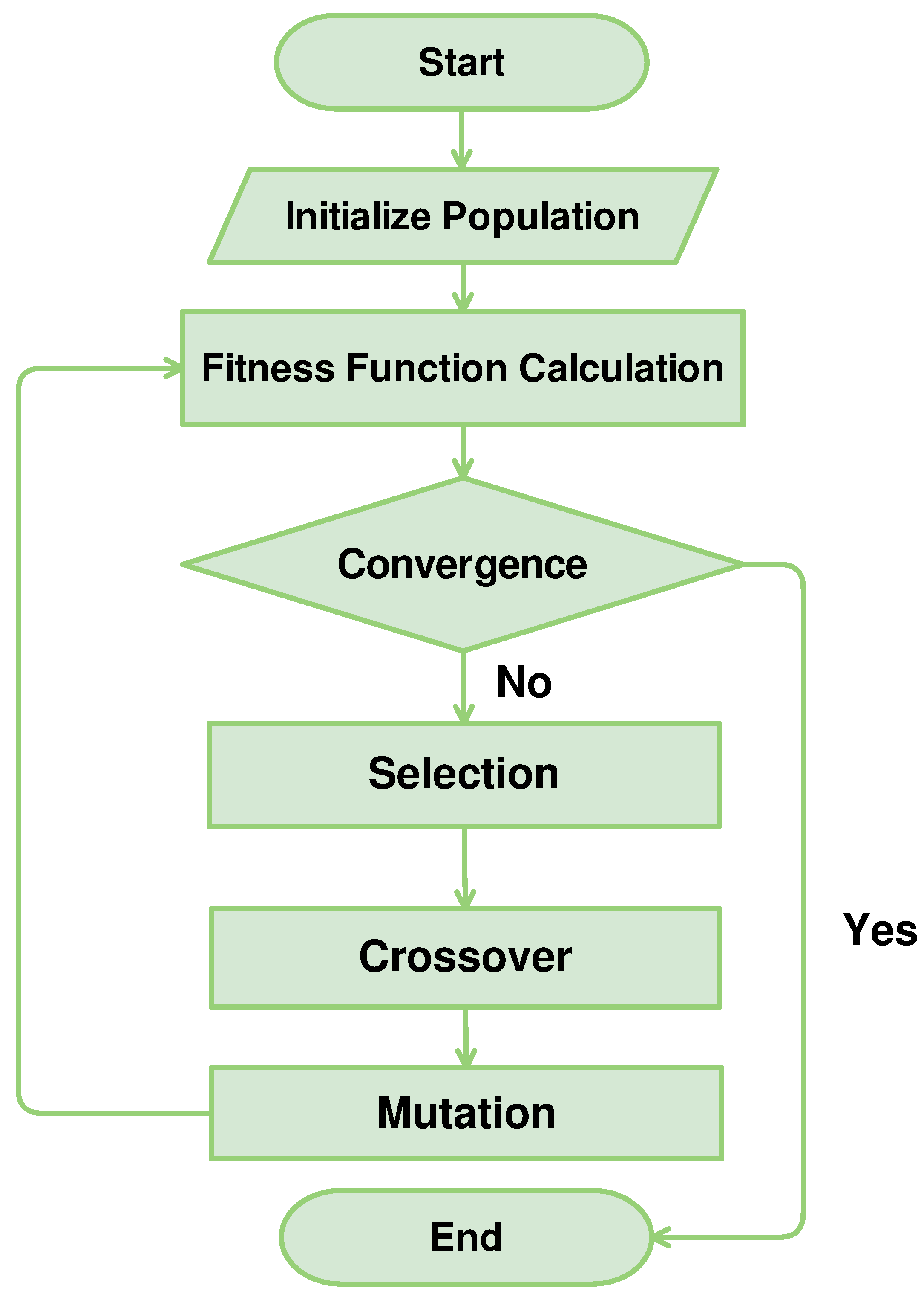
The GA methodology has been introduced by Holland [15] as a part of the computational techniques developed in the field of artificial life and complex systems [19]. The idea behind the GA is to generate high-quality solutions for optimization and search problems by applying bio-inspired operators such as mutation, crossover, and selection to a population of randomly generated candidate solutions subject to the evolutionary pressure represented by a fitness function, i.e., a functional measuring the ability of each element of the population to solve the problem. The optimal solution is computed by iterating the algorithm until the value of the fitness function converges to a equilibrium value (usually reached after 30–100 iterations). GAs have been successfully applied to a range of different fields, the most important of which are: bioinformatics, control engineering, neural networks, and medicine [16]. GAs also found applications in power systems to find optimal distributed generation (DG) placement [20], network reconfiguration to minimize losses [21], and network reconfiguration in case of failures [22]. The proposed optimization procedure is shown in the flowchart in Figure 1. The optimization procedure starts with the generation of a number of initial matrices . is a matrix, where T is the number of considered time intervals, and G is the number of generators including both ESSs and CGs. Each row of the matrix is represented by the and , which are the power profiles of the considered CGs and ESSs, respectively, during time, constructed by following the constraints given in Section 2.1. Starting from this initial population, the GA is then applied to the initial population upon satisfying a convergence criteria. Each GA iteration is organized as follows: the cost function is calculated per each element of the population. Then, selection, crossover, and mutation operators [15] are applied. In this paper, the convergence is achieved when a variability threshold of 1% or a maximum number of iterations is reached. The crossover probability has been set to , while mutation probability has been set to . Finally, when the convergence criteria are met, the optimized and are extracted from the obtained , and are chosen as a result of the optimization procedure.
2.3. Battery Cost Model
The estimation of battery operative costs is based on the battery degradation model (BDM) recently proposed by Xu et al. in [14]. The BDM is based on Equation (11), relating the battery life L with a battery degradation function . The battery life is defined as , where D is the remaining capacity of the BESS, normalized to 1. The relation among L and is non linear, and includes effects proper of the Li-ion BESSs such as the initial solid electrolyte inter-phase (SEI) film formation by means of parameters and , as given in Equation (11).
The battery degradation function depends on the sum of a calendar aging function and a cycle aging function , as given in Equation (12). Here N is the number of performed cycles.
Both calendar and cycling aging functions show a dependence on the time evolution of the operative parameters of the BESS. These are the BESS usage time , its SOC , the depth of discharge (DoD) of its performed cycles , and its temperature . In particular, the parameter can be obtained from the time evolution of the battery SOC by means of the rainflow algorithm [14].
The calendar aging function depends on the usage time and on the average SOC and temperature during the considered time interval. The dependence from these parameters is reported in Equation (13). , , and are described in Equations (14)–(16) respectively. , , , and represent the aging parameters of the Li-ion BESS analyzed and tested in [14].
Moreover, cycle aging function shows a direct dependence on the battery cycling: It depends on , average , and average temperature of the considered cycle. The expression of is given in Equation (17). The expressions of , and are given by (15), (16), and (18) respectively. The parameters , , and are obtained from [14].
The definition of calendar and cycle aging functions allows for the separate assessment of the two battery degradation phenomena. Since the calendar aging function embeds the averaging of and , the accuracy of the estimation of this phenomenon is enhanced by calculating the over sub-intervals of time length , each called . Then, the total calendar aging for a time interval has been computed as . With respect to the cycling aging, the impact of each cycle has been separately calculated as . In order to calculate the cycling pattern during the same period of time of the calendar one, it is necessary to run the rainflow algorithm on the same considered time interval . However, given the particular form of the rainflow algorithm [14], the calculated cycling patterns of two or more consecutive time intervals can differ if considered separated or as a whole, since the cycles spanning more than one interval can be truncated and not properly computed if the intervals are considered separately. For this reason, it is advisable to consider a large enough time interval during this calculation, in order to minimize the truncation error in the cycle assessment. According to this assumption, the resulting impact of the cycles performed during the time interval can be obtained as . In this way, the aging experienced by the BESS during a time interval is calculated as Equation (19).
The BDM formulation in [14] has been extended in this paper with the definition of a battery degradation cost model (BDCM). The aim has been to link the battery degradation properties with its amortization costs. Since the battery is considered degraded as it reaches a capacity D equal to 80% of its nominal value, it is possible to identify , i.e., the value of the degradation function at which the battery is considered degraded. The novel concept introduced in this paper is to consider as a linear indication of the state of degradation of the battery, which can be directly linked to a cost function. Considering that values range between 0 for a brand new battery and for a degraded one, it is possible to identify the BESS degradation during a time interval in terms of fractions of as defined in Equation (20).
Given this quantity, the BESS degradation during each considered time interval can be associated to a degradation cost . This is done by linking the amortization costs during the considered time interval with its related degradation function . Defining the total life expenses related to the BESS as , it is possible to assume the full amortization of this costs for a value of . Given the linear relation between and , it is then possible to link and by means of Equation (21):
Linking the aging of a Li-ion battery during a time interval with its amortization costs.
3. Case Study
The GA-MPOPF optimization method has been designed in order to attain high flexibility, and can be applied to a wide field of applications. In this paper, it has been applied to the planning and control strategy of a Li-ion BESS in a VPP environment. As a case study the IEEE PG & E medium voltage (MV) network, described in detail in Section 3.1, has been selected. The purpose of the VPP aggregator is to manage the power output at the point of common coupling (PCC) of the network. This is done by using the support of the BESS in order to provide a daily active power profile . If this is not achieved, the VPP aggregator is requested to pay a fine depending on the difference from the expected profile. In order to do so, the PCC of the tested grid has been treated as an infinite generator. Thus, the values and have been set to minus and plus infinite, respectively. For the same reason, no on and off switching costs of the generator have been considered. Its cost function is in the form of a constant part, depending on the profile , and a fine part depending on the fluctuations around this value, namely
The constant cost function follows the day-ahead market prices, and the fines cost functions are chosen among the ones shown in Section 3.2.
3.1. The Test Grid
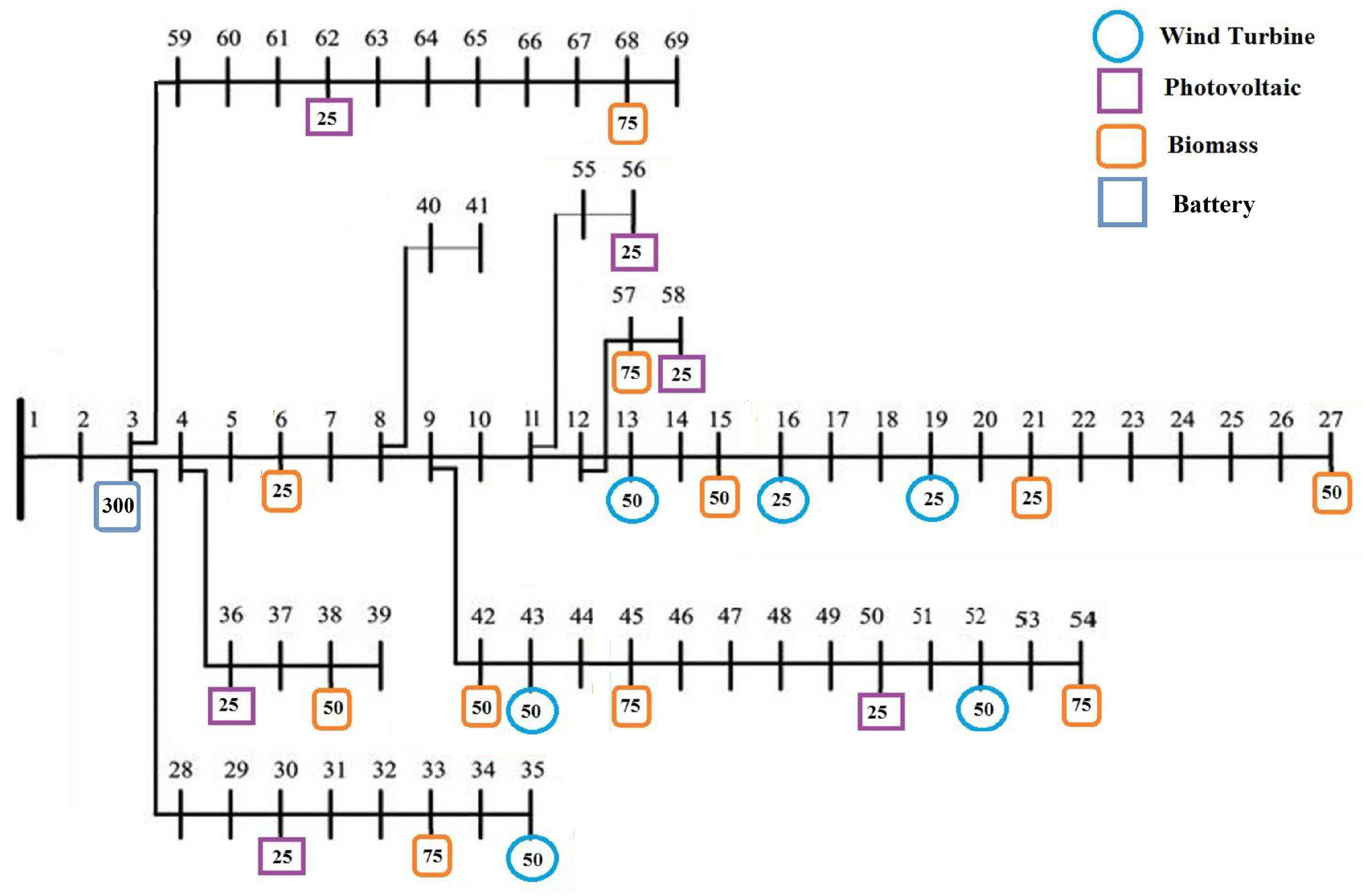
The standard PG & E 69-bus radial distribution network used in [23] is selected and reported in Figure 2. The information regarding DG has been taken from [24,25], where the authors optimized DG position and nominal power in order to stabilize the network by using a heuristic, Tabu Search-based algorithm. The load data has been obtained by using the methodology described in [26], where the consumption profiles of medium voltage nodes are aggregated randomly, starting from a set of consumption time series of single households obtained from [26]. Following this procedure, the load profile of each node of the network has been estimated, with hourly sampling and for a period of a month. The time profiles of the DG production considered in this study have been collected from the website of IESO, the power system operator based in Ontario (Canada) [27]. The tested Li-ion BESS has a capacity of 300 kWh and a rated power of 300 kW. All the datasets used in this paper cover the period from April to May 2016.
3.2. Cost Functions
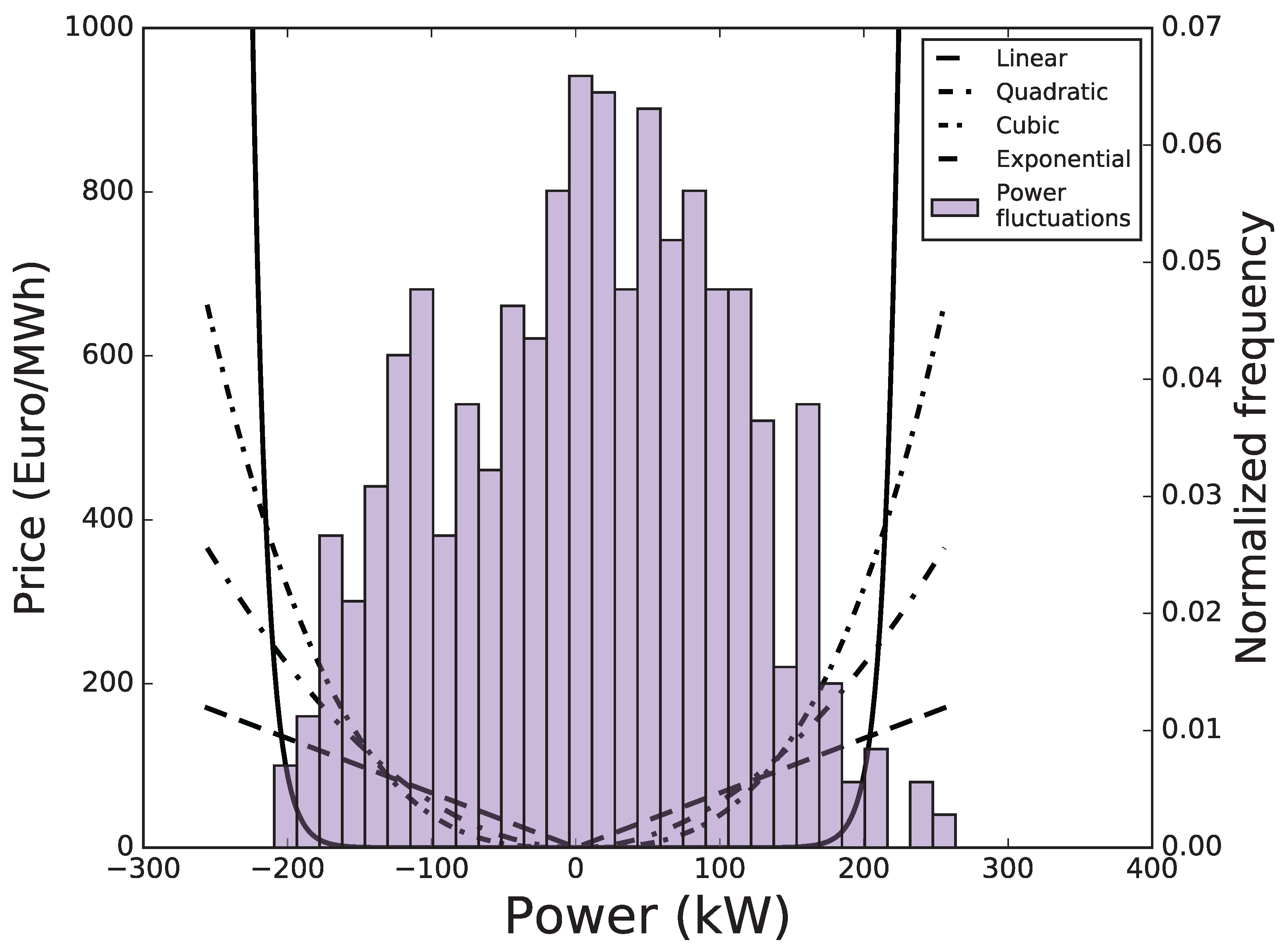
The optimization procedure proposed in Section 2 has been tested according to four different types of fine cost functions : linear, quadratic, cubic, and exponential, described respectively in (23)–(26). The first three of them have been chosen as representative cost functions in power generation [17]. The exponential one has been proposed in this paper as a limit case for testing the algorithm response for cost functions of higher grade. The intensity of the fines is tuned by the parameter , which is different per each cost function, and defined in order to obtain an average fine of EUR/MWh.
Figure 3 reports the shape of the tested cost functions. Moreover, the proposed cost functions are compared with the histogram of the power fluctuations observed in the PCC with respect to the power profile . Fluctuations are distributed around the interval kW, with some extreme values between 200 and 300 kW.
4. Results
The GA-MPOPF method is used to optimize the usage of a BESS in a VPP, as described in detail in Section 3.
Aim of the optimization is therefore to select the best option between the usage (and subsequent degradation) of the BESS and the payment of the fines due to the VPP power fluctuations around the selected equilibrium value . Ideally, the proposed procedure will choose the best combinations of these two factors from an economic point of view and during an extended period of time, ensuring that the electrical constraints of the grid are met during the full time interval. In the tested case, has been chosen as a daily flat value, equal to the average balance of the network during the day. The following results have been obtained by setting the total life expenses related to the BESS as , where is the nominal capacity of the BESS, and EUR/kWh is the BESS overnight cost per unity of capacity. The average fine cost has been set to EUR/MWh.
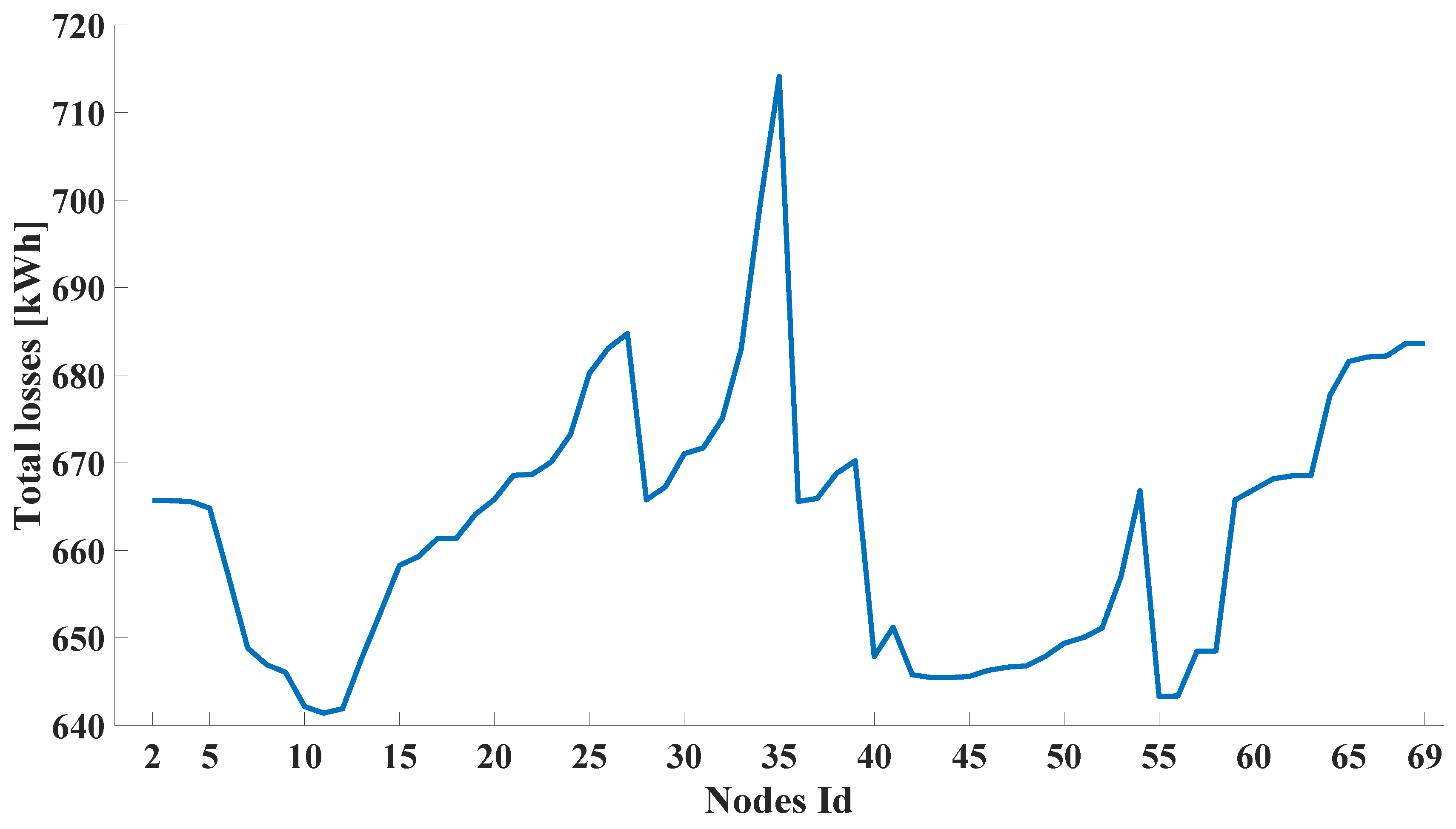
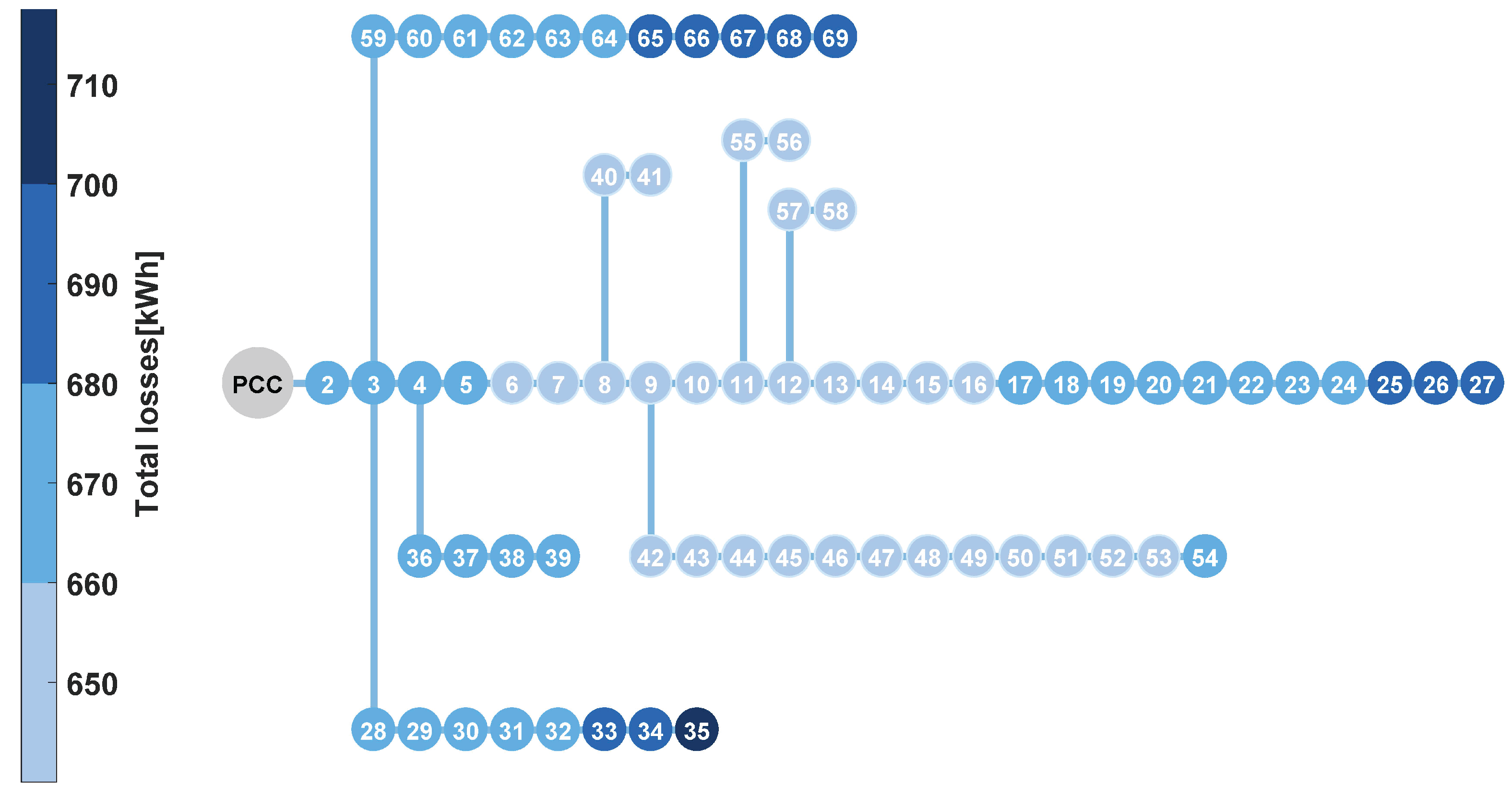
The proposed methodology has been applied for the planning procedure involving the correct positioning of the considered BESS. In order to do so, the effects of the tested BESS have been evaluated by simulating the presence of the optimized BESS in one bus of the system. The procedure has been replicated per each node of the network, in order to compare the impact of the BESS position on the operating parameters. As first result, it has been found that all the system constraints given in Section 2 are met for every considered time interval and for every position of the BESS. This high stability of the network is due to two factors: the presence of household users only, and the study of the optimal positioning of DG performed in [24]. For this reason, no considerations regarding the system voltage phasors and thermal limits should be taken for defining the correct positioning of the BESS. However, the proposed methodology would be able to include these parameters in the planning procedure in case of potentially unstable grids. Moreover, the GA-MPOPF allowed for the estimation of the system losses with respect to the different positioning of the BESS. The results of this procedure are given in Figure 4 and Figure 5. The values associated to each node n represent the monthly losses of the system when the BESS is positioned on the node itself. Values are given in kWh. The best placement of the BESS has been found to be at node 11.
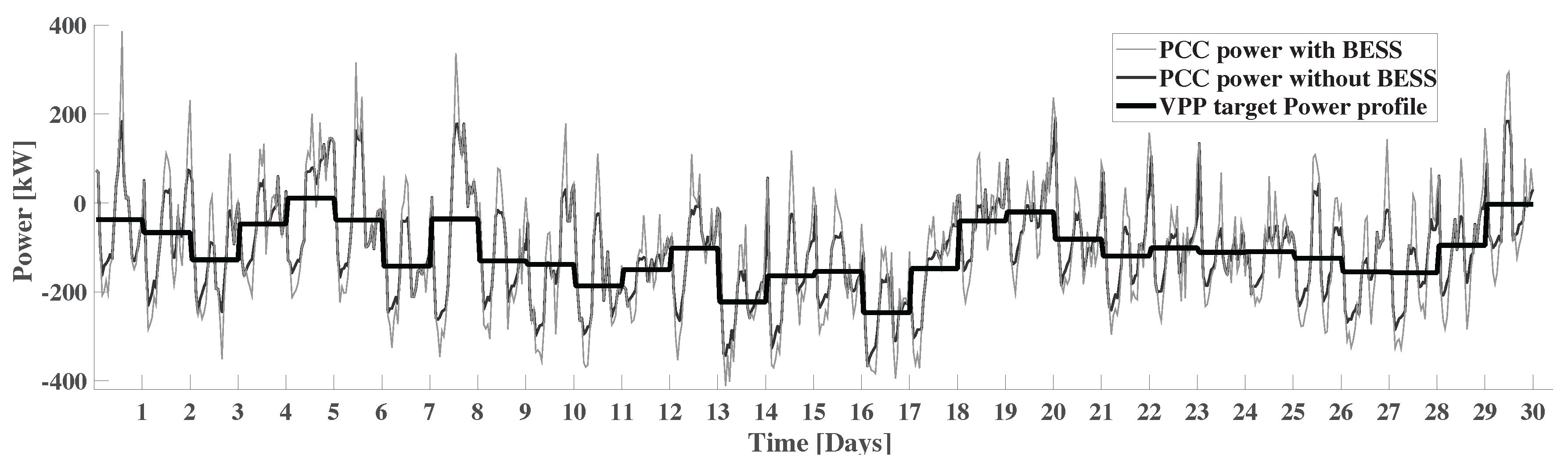
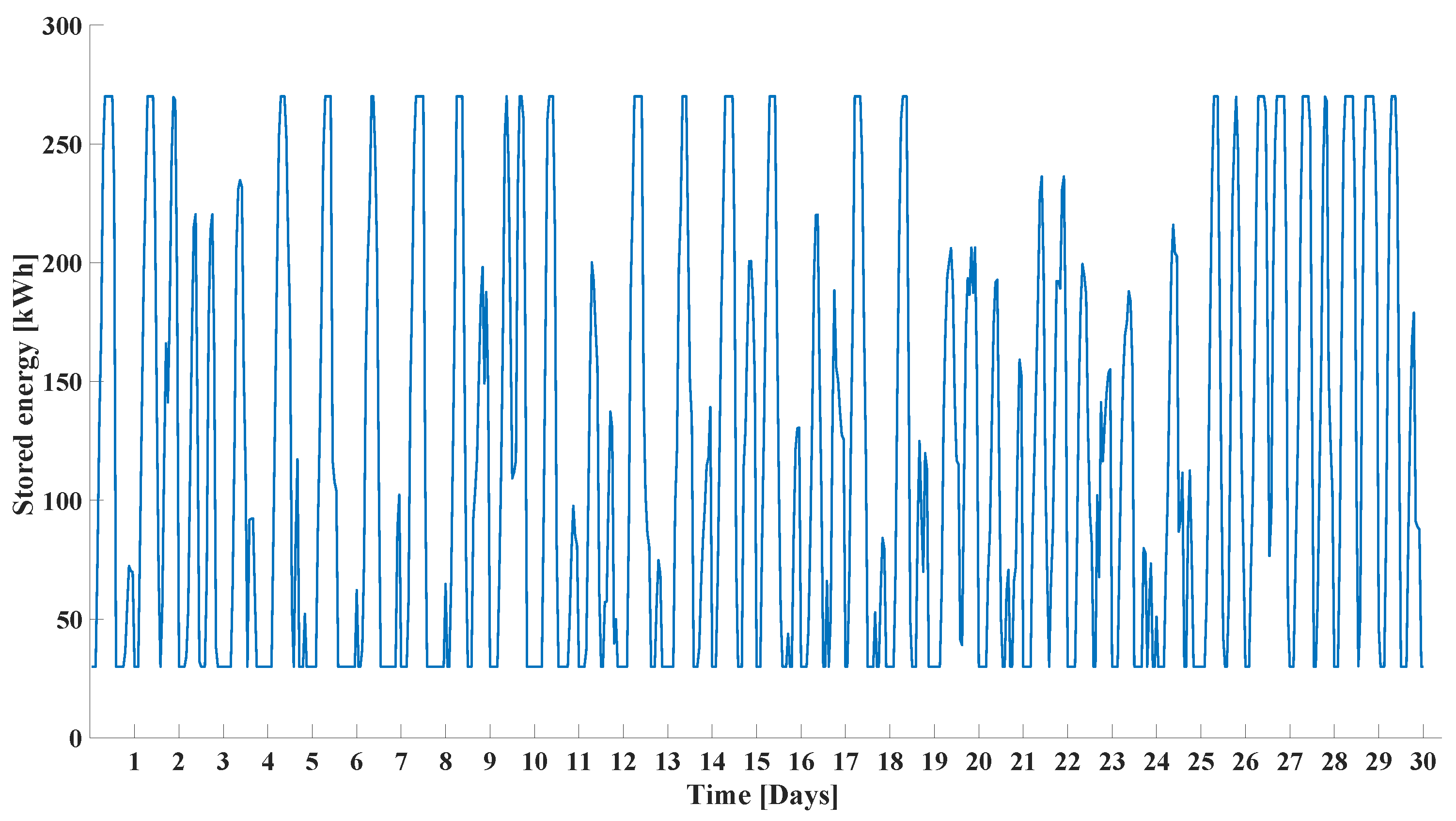
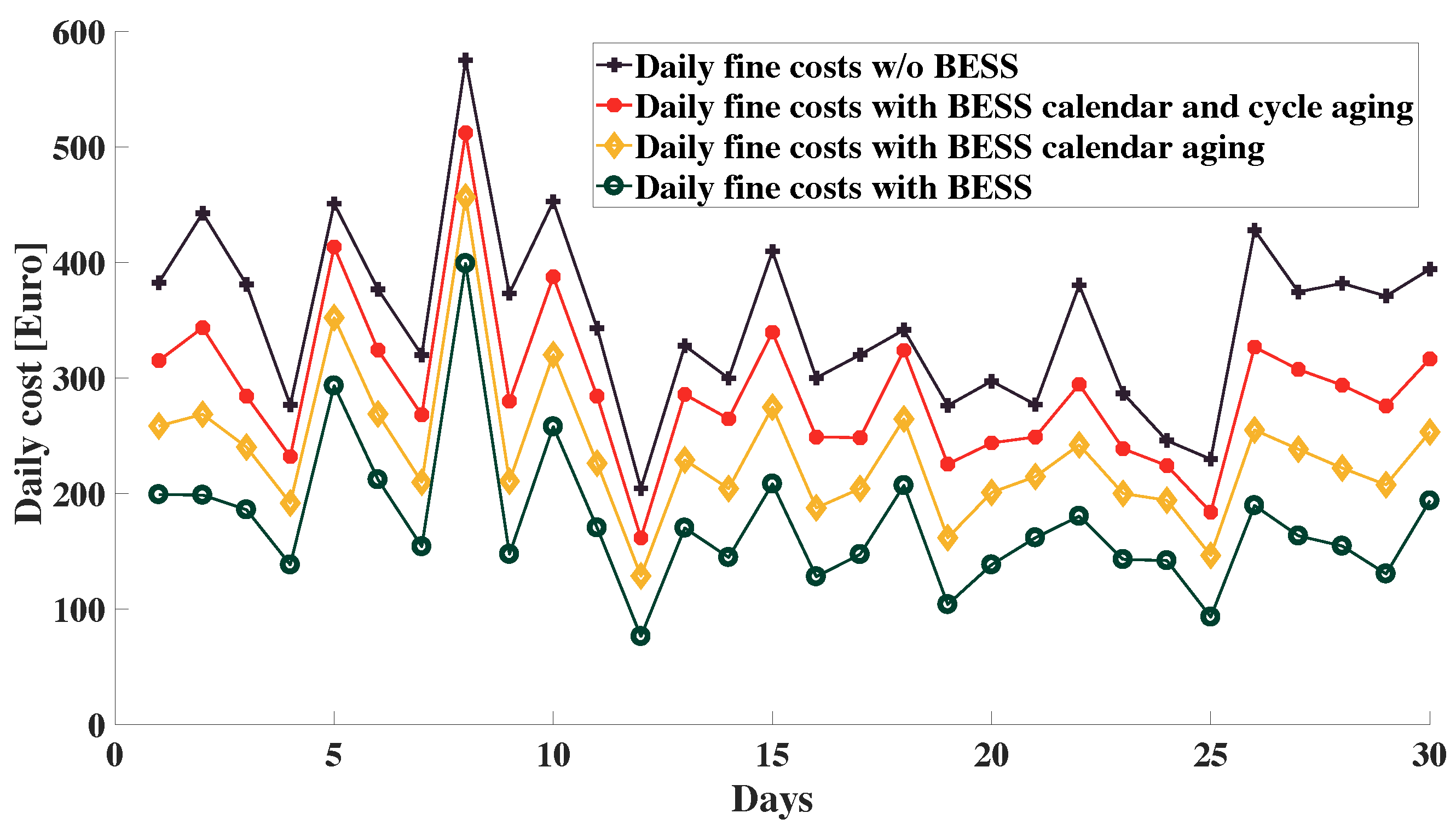
Once identified the best positioning of the BESS, it was possible to estimate the economic impact of the BESS on the system. Figure 6 and Figure 7 show the optimization results for the studied month, in the case of quadratic cost fines, and for the positioning of the BESS on node 11. Also, Figure 6 shows the power output at the PCC of the tested VPP. This result is shown both in presence and in absence of the BESS for the quadratic cost function. Also, Figure 7 shows the SOC profile of the BESS during the tested month. Figures show how, depending on the particular shape of the system power fluctuations, the optimized number of daily full cycles is between zero and two, with the presence of common BESS micro-cycles. Moreover, Figure 8 shows the daily costs resulting from the monthly optimization. In particular, the black line shows the reference fines cost value of the system without the BESS, the green line shows the system fines in presence of the BESS, and the orange and red lines show the cumulative cost of fines and calendar aging, and the cumulative cost of fines, calendar and cycle aging, respectively. The latter represents the total cost of the studied system in the presence of the BESS. These costs have been calculated on top of the monthly optimization by following the procedure given in Section 2. The calendar aging impact has been computed by setting a time window per each considered day, whereas the daily cycling aging impact has been calculated by considering all the cycles performed in the considered day. In the case in which one or more considered cycles spanned over more than one day, the amortization cost of the cycle has been divided among the days accordingly, to the ratio between the time that the cycle spanned during the considered days and the total cycle length. Also, the result regarding the system costs cumulated on a monthly base is given in Table 1, while the total monthly energy fluctuations at the PCC level are given in Table 2. As a result, the optimized use of the BESS shows a reduction in the fine cost ranging between 30% and 60% on a daily basis, if compared to the fine cost in absence of the BESS. The same result computed on a monthly basis leads to a fine cost reduction of 50%. Since both the BESS calendar and cycle aging showed a daily amortization cost ranging between 10% and 15% of the daily fines in absence of the BESS, this translated to a reduction of the system amortization costs ranging between 10% and 25%. The same quantity calculated on a monthly basis showed a reduction in the system total costs of 18%.
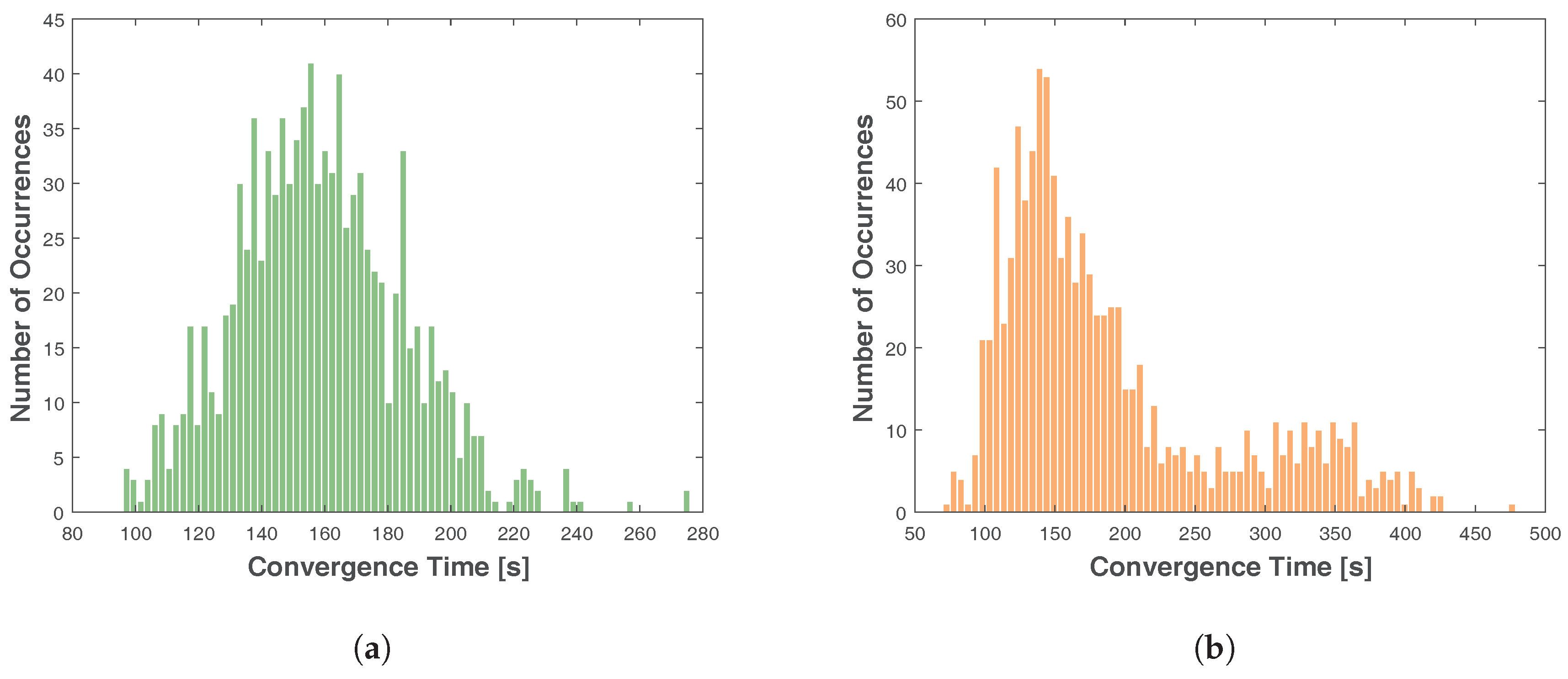
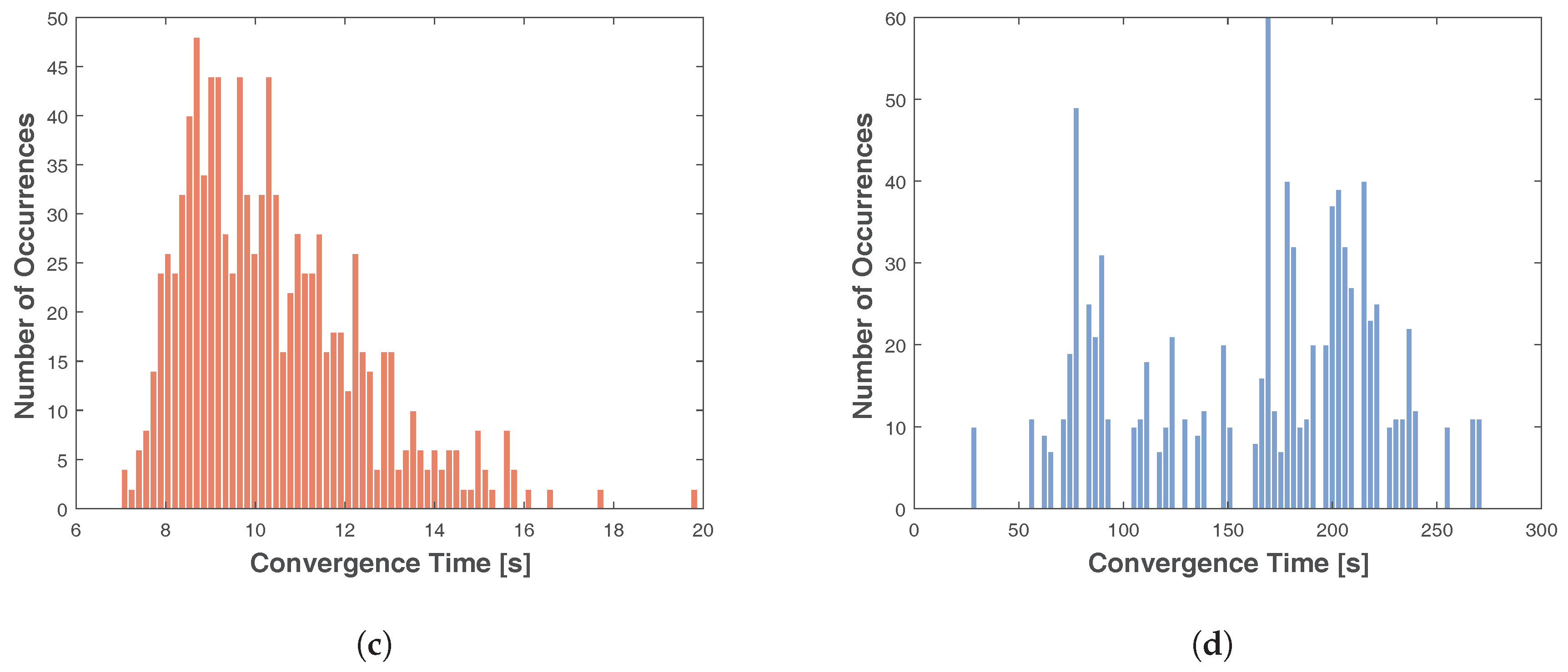
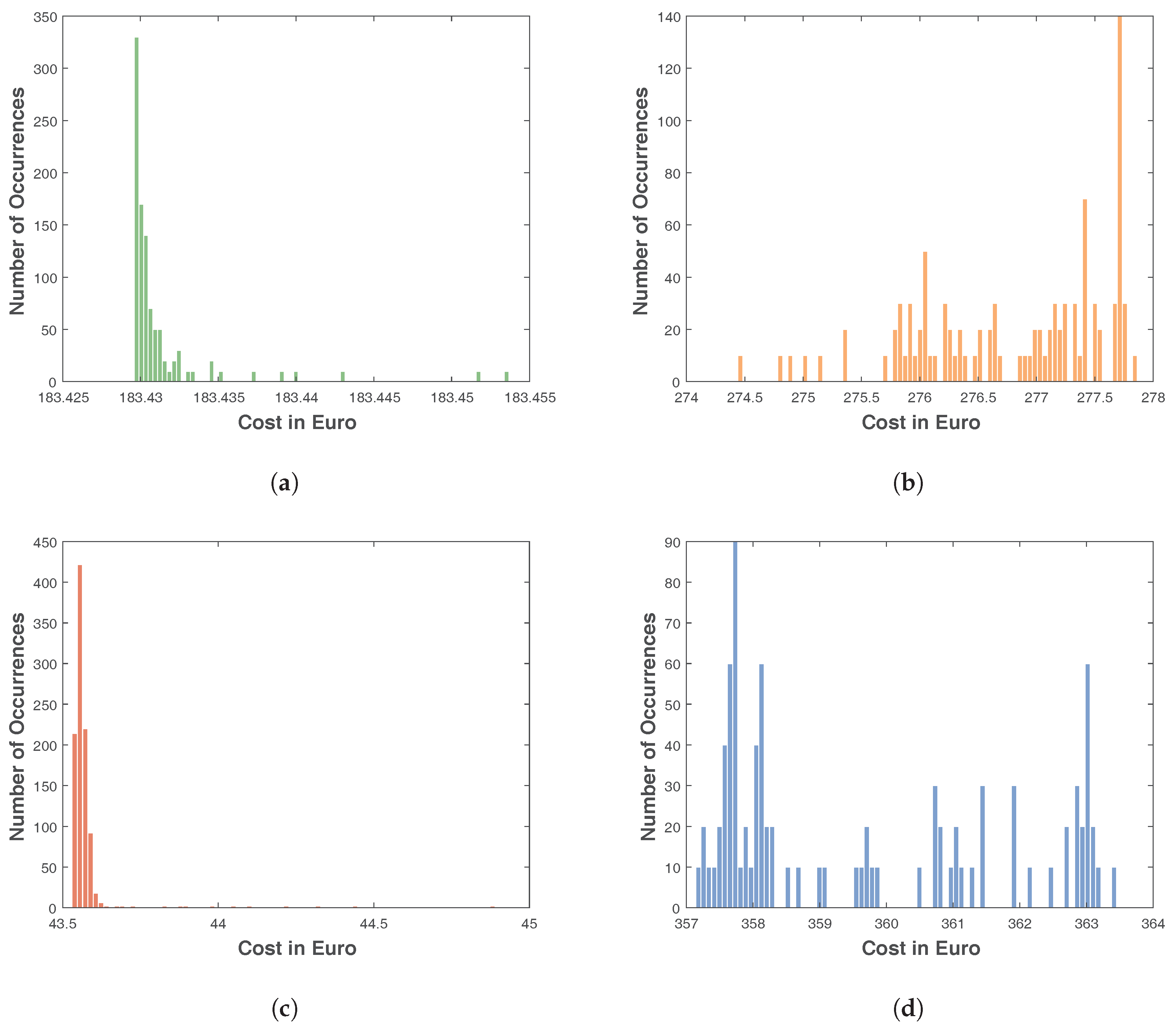
With regard to the algorithmic performance, Figure 9 and show the convergence properties of the proposed GA-MPOPF. Since the GA procedure involves random sampling of the phase space, the results of different optimization runs performed on the same system configuration can differ, possibly providing different outcomes regarding the final optimized fitness function and the running time. In order to identify the impact of this random sampling and estimate the convergence properties of this stochastic procedure, the optimization procedure has been replicated for 1000 times in the same time interval. Then, the obtained daily optimal costs and running times are plotted as histograms. Figure 9 shows the histograms of the optimal costs and Figure 10 shows the histograms of the running time. In order to investigate the different convergence properties of the algorithm for different types of cost functions, the same procedure has been applied for the cost functions described in Section 3. In particular, the results shown in Figure 9 highlight that all the cost functions show a relative convergence error under 1.5%. Cubic and exponential cost functions show even better convergence properties, of the order of 0.2% and 0.1%, respectively. This is due to the particular shape of the cost functions, depicted in Figure 3. In fact, both the cubic and the exponential cost functions show a flat cost for small power fluctuations. For this reason, the usage of the battery in the flat area is not economically advantageous. Since the usage of the BESS is economically forbidden in this areas for cubic and exponential cost functions, the optimization easier to achieve.
As results, the algorithm shows excellent convergence properties for all types of cost functions.
5. Discussion
The results regarding the BESS positioning are given in Figure 4 and Figure 5. The figures show how the correct positioning of the BESS in this system can save up to 10% of losses on a monthly scale. From a systemic perspective, the best positioning of the BESS has been found to be in the topological center of the grid, in node 11. As shown in Figure 5, the positioning of the BESS on the surrounding nodes has been proven to be a good choice. The greater is the distance from this point, the more the losses have been shown to increase.
Concerning the results of the optimization given in Figure 6, Figure 7 and Figure 8, the algorithm has been found to be reliable in limiting high power fluctuations, showing non-trivial management decisions in the case of fluctuations over periods of time of various hours, possibly leading to an high fine for the aggregator. In order to reduce these fines, the algorithm decided to split the available energy capacity of the BESS during the full interval. Moreover, it is important to notice how small fluctuations are not compensated by the usage of the BESS, since the fines associated to them are lower than the cycling aging costs of the BESS. This effect is clear when Figure 6, Figure 7 and Figure 8 are compared: the days characterized by small power fluctuations show wasted BESS capacity and low cycling costs, due to the limited use of the BESS.
Finally, looking at the behavior of the system in the presence of relevant power peaks, it is possible to notice how the battery energy is almost totally used for reducing the high fluctuation events. This is due to the quadratic shape of the fine cost function, which forces the algorithm to give priority to high fluctuations. In particular, the power requested at PCC level in presence of the highest peaks is reduced by a value between 30% and 50%. The effect of this reduction clearly impacts on the daily system costs. This is evident when comparing Figure 6 and Figure 8 on the days in which the highest fluctuations are present around the mean value. In particular, these are days 2, 5, 8, 10, 15, 22 and 26. Especially on days 2, 8 and 26, it it clearly visible how the fine cost is reduced by approximately 60% by using the BESS. By comparing this values carefully, such a large reduction in fines costs is proper of the days in which it is possible to observe consistent fluctuations in power. These periods do not last for more than two-three hours. If these last longer, as in the case of day 8, the reduction in the fine costs due to the presence of the BESS is reduced to a value of around 30%.
The cost results of the optimization are compared with the existing literature, and in particular with papers which assess the cost impact of ESSs using MPOPF methods and quadratic cost functions for balancing generation [8,11]. The resulting cost reduction obtained in [11] ranges between 40% and 50%, with respect to the cost of the system without ESS. In the study performed in [8], the authors identified an improvement in cost of around 10% with respect to the case without ESS. Neither paper specified the type of considered ESS, and did not consider any aging cost for them. In any case, it is possible to compare their results with the ones presented here, without considering the BESS aging costs. In this particular case, the findings of the present papers agree with the ones in [11], as well as showing better cost improvements than the ones found in [8].
6. Conclusions
This paper presents a multi-period optimal power flow methodology based on genetic algorithms. The proposed methodology is designed for the optimization of both planning and unit-commitment problems in presence of ESSs and fluctuations induced by distributed RESs, and is able to take into account the costs related to the aging of the considered ESSs. As a test case, it has been applied to an IEEE prototypical test network aiming to work as a VPP by means of the usage of a Li-ion battery. The tested methodology has been used for two different applications: a first, planning application, involving the definition of the correct positioning of the BESS in the system; and a second, operative one, involving the definition of the correct BESS control strategy. Moreover, a convergence analysis of the proposed algorithm is presented. Four cost function models (linear, exponential, quadratic, and cubic) have been considered for this analysis.
Results put in evidence the importance of the GA-based multi-period optimization method when dealing with ESSs. In particular, the proposed methodology has been found to be able to deal with complex decision criteria regarding the optimal management of both the cycle aging costs and the SOC profile of the BESS. Moreover, the proposed method has shown the ability to deal with longer time spans with respect to the methodologies proposed in literature, going beyond the usual time scales between one day and one week, proving to be able to optimize dataset even in case of monthly time scales. This allowed its application for planning procedures. Also, a comparison of the results of the proposed methodology with similar ones present in literature highlights the importance in considering the ESS aging costs during the economic optimization. In particular, results show that including aging costs can significantly change the quantitative result of the economic assessment. Since the amortization costs due to BESS aging represent a fraction between 40% and 60% of the total system costs, failing to take them into account can lead to a significant underestimation of the costs. On the other hand, the analysis performed in this paper confirmed the economic advantage associated to the installation of a BESS, for the investigated purposes.
Also, a convergence analysis of the proposed GA-MPOPF showed excellent convergence properties when converging to the optimal cost, even in the special case of the exponential cost function (i.e., when using ESSs it is not favorable because of the lower cost of the fine). This allowed the identification of the different responses of BESSs for different fine systems.
In general, the use of genetic algorithms provides the user with the advantage of a flexible and fully configurable tool both from a technical and economic point of view. This is highlighted by the results regarding the algorithm convergence properties, which have shown excellent and fast convergence even in the case of nonlinear constraints and nonlinear objective functions.
Future research will be devoted to the application of the method to a broadest spectrum of problems, including ESS sizing optimization in power systems of sizes ranging from microgrids to national transmission systems.
Acknowledgments
This work was developed within the project NETfficient, “Energy and Economic Efficiency for Today’s Smart Communities through Integrated Multi Storage Technologies”. This project has received funding from the European Union’s Horizon 2020 research and innovation programme under grant agreement No. 646463.
Author Contributions
All authors conceived and designed the experiments; Saman Korjani performed the experiments; All authors analyzed the data and wrote the paper; Alfonso Damiano supervised the research activities.
Conflicts of Interest
The authors declare no conflict of interest.
Abbreviations
The following abbreviations are used in this manuscript:
| ESS | Energy Storage System |
| BESS | Battery Energy Storage System |
| RES | Renewable Energy Sources |
| MPOPF | Multi-Period Optimal Power Flow |
| GA | Genetic Algorithm |
| GA-MPOPF | Genetic Algorithm-based Multi Period Optimal Power Flow |
| SOC | State Of Charge |
| VPP | Virtual Power Plant |
| BDM | Battery Degradation Model |
| BDCM | Battery Degradation Costs Model |
| CG | Controllable Generator |
| MV | Medium Voltage |
| PCC | Point of Common Coupling |
References
- Facchini, A. Distributed energy resources: Planning for the future. Nat. Energy 2017, 2, 17129. [Google Scholar] [CrossRef]
- Marongiu, A.; Damiano, A.; Heuer, M. Experimental analysis of lithium iron phosphate battery performances. In Proceedings of the 2010 IEEE International Symposium on Industrial Electronics, Bari, Italy, 4–7 July 2010; pp. 3420–3424. [Google Scholar]
- Beltran, H.; Bilbao, E.; Belenguer, E.; Etxeberria-Otadui, I.; Rodriguez, P. Evaluation of Storage Energy Requirements for Constant Production in PV Power Plants. IEEE Trans. Ind. Electron. 2013, 60, 1225–1234. [Google Scholar] [CrossRef]
- Haddadian, G.; Khalili, N.; Khodayar, M.; Shahidehpour, M. Optimal scheduling of distributed battery storage for enhancing the security and the economics of electric power systems with emission constraints. Electr. Power Syst. Res. 2015, 124, 152–159. [Google Scholar] [CrossRef]
- Ghofrani, M.; Arabali, A.; Etezadi-Amoli, M.; Fadali, M.S. A Framework for Optimal Placement of Energy Storage Units within a Power System with High Wind Penetration. IEEE Trans. Sustain. Energy 2013, 4, 434–442. [Google Scholar] [CrossRef]
- D’Agostino, R.; Baumann, L.; Damiano, A.; Boggasch, E. A Vanadium-Redox-Flow-Battery Model for Evaluation of Distributed Storage Implementation in Residential Energy Systems. IEEE Trans. Energy Convers. 2015, 30, 421–430. [Google Scholar]
- Mureddu, M.; Damiano, A. A statistical approach for resilience analysis of ESS deployment in RES-based power systems. In Proceedings of the 2017 IEEE 26th International Symposium on Industrial Electronics (ISIE), Edinburgh, UK, 19–21 June 2017; pp. 2069–2074. [Google Scholar]
- Gayme, D.; Topcu, U. Optimal power flow with distributed energy storage dynamics. In Proceedings of the 2011 American Control Conference, San Francisco, CA, USA, 29 June–1 July 2011; pp. 1536–1542. [Google Scholar]
- Warrington, J.; Goulart, P.; Mariethoz, S.; Morari, M. Policy-Based Reserves for Power Systems. IEEE Trans. Power Syst. 2013, 28, 4427–4437. [Google Scholar] [CrossRef]
- Gopalakrishnan, A.; Raghunathan, A.U.; Nikovski, D.; Biegler, L.T. Global optimization of multi-period optimal power flow. In Proceedings of the 2013 American Control Conference, Washington, DC, USA, 17–19 June 2013; pp. 1157–1164. [Google Scholar]
- Jabr, R.A.; Karaki, S.; Korbane, J.A. Robust Multi-Period OPF With Storage and Renewables. IEEE Trans. Power Syst. 2015, 30, 2790–2799. [Google Scholar] [CrossRef]
- Rabiee, A.; Parniani, M. Voltage security constrained multi-period optimal reactive power flow using benders and optimality condition decompositions. IEEE Trans. Power Syst. 2013, 28, 696–708. [Google Scholar] [CrossRef]
- Scott, P.; Thiébaux, S. Distributed Multi-Period Optimal Power Flow for Demand Response in Microgrids. In Proceedings of the 2015 ACM Sixth International Conference on Future Energy Systems (e-Energy’15), Bangalore, India, 14–17 July 2015; pp. 17–26. [Google Scholar]
- Xu, B.; Oudalov, A.; Ulbig, A.; Andersson, G.; Kirschen, D. Modeling of Lithium-Ion Battery Degradation for Cell Life Assessment. IEEE Trans. Smart Grid 2016, 28, 1–1. [Google Scholar] [CrossRef]
- Holland, J.H. Adaptation in Natural and Artificial Systems; MIT Press: Cambridge, MA, USA, 1992. [Google Scholar]
- Chambers, L. The Practical Handbook of Genetic Algorithms: Applications, 2nd ed.; Chapman&Hall/CRC: London, UK, 2000. [Google Scholar]
- Zimmerman, R.D.; Murillo Sanchez, C.; Thomas, R. MATPOWER: Steady-State Operations, Planning, and Analysis Tools for Power Systems Research and Education. IEEE Trans Power Syst. 2011, 26, 12–19. [Google Scholar] [CrossRef]
- Chang, G.W.; Chu, S.Y.; Wang, H.L. An Improved Backward/Forward Sweep Load Flow Algorithm for Radial Distribution Systems. IEEE Trans. Power Syst. 2007, 22, 882–884. [Google Scholar] [CrossRef]
- Langton, C.G. Atificial Life: An Overview; MIT Press: Cambridge, MA, USA, 1997. [Google Scholar]
- Georgilakis, P.; Hatziargyriou, N. Optimal distributed generation placement in power distribution networks: Models, methods, and future research. IEEE Trans. Power Syst. 2013, 28, 3420–3428. [Google Scholar] [CrossRef]
- Cebrian, J.C.; Kagan, N. Reconfiguration of distribution networks to minimize loss and disruption costs using genetic algorithms. Electr. Power Syst. Res. 2010, 80, 53–62. [Google Scholar] [CrossRef]
- Lu, T.; Wang, Z.; Ai, Q.; Lee, W.J. Interactive Model for Energy Management of Clustered Microgrids. IEEE Trans. Ind. Appl. 2017, 9994, 1739–1750. [Google Scholar] [CrossRef]
- Baran, M.E.; Wu, F.F. Optimal capacitor placement on radial distribution systems. IEEE Trans. Power Deliv. 1989, 4, 725–734. [Google Scholar] [CrossRef]
- Arefifar, S.A.; Mohamed, Y.A.R.I.; El-Fouly, T.H.M. Supply-adequacy-based optimal construction of microgrids in smart distribution systems. IEEE Trans. Smart Grid 2012, 3, 1491–1502. [Google Scholar] [CrossRef]
- Arefifar, S.A.; Mohamed, Y.A.R.I.; El-Fouly, T.H.M. Optimum microgrid design for enhancing reliability and supply-security. IEEE Trans. Smart Grid 2013, 4, 1567–1575. [Google Scholar] [CrossRef]
- Malekpour, A.R.; Pahwa, A. Radial Test Feeder including primary and secondary distribution network. In Proceedings of the 2015 North American Power Symposium (NAPS), Charlotte, NC, USA, 4–6 October 2015; pp. 1–9. [Google Scholar]
- IESO. 2017. Available online: http://ieso.ca/ (accessed on 15 May 2017).
Figure 1.
The flowchart of the genetic algorithm.

Figure 2.
The used IEEE PG & E 69 bus network.

Figure 3.
The used cost functions, and the histogram of the power fluctuations at the network point of common coupling (PCC).
Figure 3.
The used cost functions, and the histogram of the power fluctuations at the network point of common coupling (PCC).

Figure 4.
Monthly energy losses for different positioning of the battery energy storage system (BESS).
Figure 4.
Monthly energy losses for different positioning of the battery energy storage system (BESS).

Figure 5.
Monthly energy losses associated to each different location of the BESS. The losses are given by means of a color code, described in the legend.
Figure 5.
Monthly energy losses associated to each different location of the BESS. The losses are given by means of a color code, described in the legend.

Figure 6.
The power profile at the PCC of the considered virtual power plant (VPP), in both presence and absence of a BESS.
Figure 6.
The power profile at the PCC of the considered virtual power plant (VPP), in both presence and absence of a BESS.

Figure 7.
The time evolution of the energy stored in the considered BESS.

Figure 8.
The daily cost of the system. The fine cost and the BESS calendar and cycling aging amortization costs are given as a sum. Also, the daily fine cost of the system without the BESS is given as a reference.
Figure 8.
The daily cost of the system. The fine cost and the BESS calendar and cycling aging amortization costs are given as a sum. Also, the daily fine cost of the system without the BESS is given as a reference.

Figure 9.
Histograms of the convergence of the total cost considering the four different tested cost functions. (a) Cubic cost function; (b) Quadratic cost function; (c) Exponential cost function; (d) Linear cost function.
Figure 9.
Histograms of the convergence of the total cost considering the four different tested cost functions. (a) Cubic cost function; (b) Quadratic cost function; (c) Exponential cost function; (d) Linear cost function.

Figure 10.
Histograms of the running time for different cost functions. (a) Cubic cost function; (b) Quadratic cost function; (c) Exponential cost function; (d) Linear cost function.
Figure 10.
Histograms of the running time for different cost functions. (a) Cubic cost function; (b) Quadratic cost function; (c) Exponential cost function; (d) Linear cost function.

Table 1.
Comparison of monthly costs with and without a BESS.
| Monthly Considered Costs | Costs (Euro) | Cumulative Costs (Euro) |
|---|---|---|
| Fines with a BESS | 5200 | 5200 |
| Calendar aging | 1800 | 7000 |
| Cycling aging | 1700 | 8700 |
| Fines w/o a BESS | 10,500 | 10,500 |
Table 2.
Comparison of monthly energy fluctuations at the PCC level with and without a BESS.
| Type | Energy (MWh) |
|---|---|
| With a BESS | 49.7 |
| Without a BESS | 70.2 |
© 2017 by the authors. Licensee MDPI, Basel, Switzerland. This article is an open access article distributed under the terms and conditions of the Creative Commons Attribution (CC BY) license (http://creativecommons.org/licenses/by/4.0/).
Share and Cite
MDPI and ACS Style
Korjani, S.; Mureddu, M.; Facchini, A.; Damiano, A. Aging Cost Optimization for Planning and Management of Energy Storage Systems. Energies 2017, 10, 1916. https://doi.org/10.3390/en10111916
AMA Style
Korjani S, Mureddu M, Facchini A, Damiano A. Aging Cost Optimization for Planning and Management of Energy Storage Systems. Energies. 2017; 10(11):1916. https://doi.org/10.3390/en10111916
Chicago/Turabian StyleKorjani, Saman, Mario Mureddu, Angelo Facchini, and Alfonso Damiano. 2017. "Aging Cost Optimization for Planning and Management of Energy Storage Systems" Energies 10, no. 11: 1916. https://doi.org/10.3390/en10111916
Note that from the first issue of 2016, this journal uses article numbers instead of page numbers. See further details here.