Operational Range of Several Interface Algorithms for Different Power Hardware-In-The-Loop Setups

Abstract

The importance of Power Hardware-in-the-Loop (PHIL) experiments is rising more and more over the last decade in the field of power system and components testing. Due to the bidirectional exchange between virtual and physical systems, a true-to-reality interface is essential; however, linking several dynamic systems, stability issues can challenge the experiments, the components under test, and the individuals performing the experiments. Over the time, several interface algorithms (IA) have been developed and analyzed, each having different advantages and disadvantages in view of combining virtual simulations with physical power systems. Finally, IA are very specific to the kind of PHIL experiment. This paper investigates the operational range of several IA for specific PHIL setups by calculations, simulations, and measurements. Therefore, a selection of the mainly used respectively optimized IA is mathematically described. The operational range is verified in a PHIL system testing environment. Furthermore, in order to study the influence of different PHIL setups, according to software and hardware impedance, different tests using linear and switching amplifiers are performed.

1. Introduction

Challenging global goals for decentralized energy resources integration [1] lead on the one hand to the improvement of energy efficiency and the decrease of CO₂ emissions and, on the other hand, to the reduction of development costs and time for new smart grid components. Power Hardware-in-the-Loop (PHIL) technologies are present in the field of component testing, in power system stability studies as risk-free alternative for field tests (or preliminary testing), and are supporting the verification of new control strategies [2,3].

Nonetheless, by running realistic and stable experiments by bidirectional connection of a virtual simulated system (VSS) with a physical power system (PPS), an interface algorithm (IA) has to be used to eliminate inaccuracies and disturbances that result from the necessary coupling of devices like power amplifiers and measurement probes [4,5].

For the interaction between physical and virtual power domains, a power adaptive coupling element is needed. Considering this aspect, this paper will concentrate on the use of linear or switching amplifiers, which adapt control signals from the VSS to the necessary level of the PPS and is furthermore acting as a power sink or source.

In addition to physical connections via amplifiers in a testing environment, further software adaptions need to be made in order to perform secure and stable experiments. For this purpose, different IA are analyzed and compared.

The paper is structured as an overview of already existing IA studies on different laboratory setups. The results can be used to simplify preliminary stability studies of new PHIL testbeds and planned PHIL experiments by the choice of the most suitable IA.

2. Interface Algorithms of Power Hardware-In-The-Loop Systems

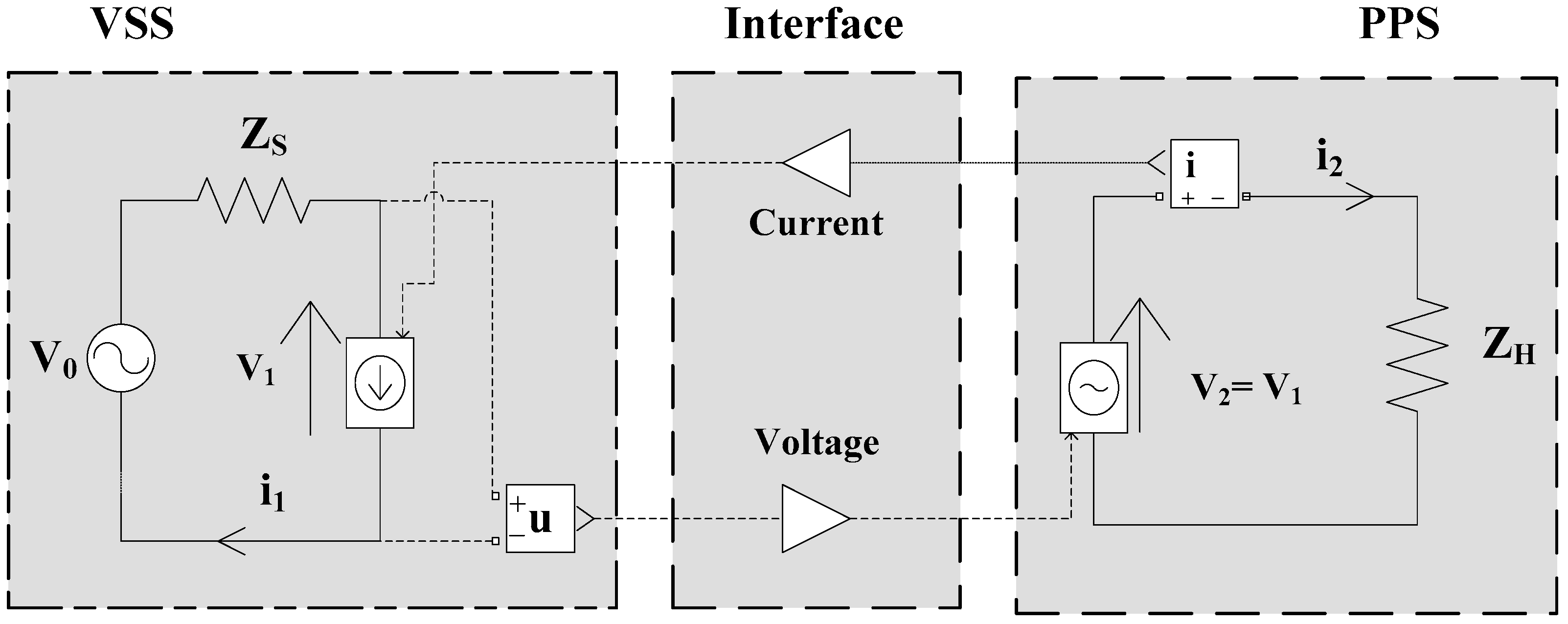
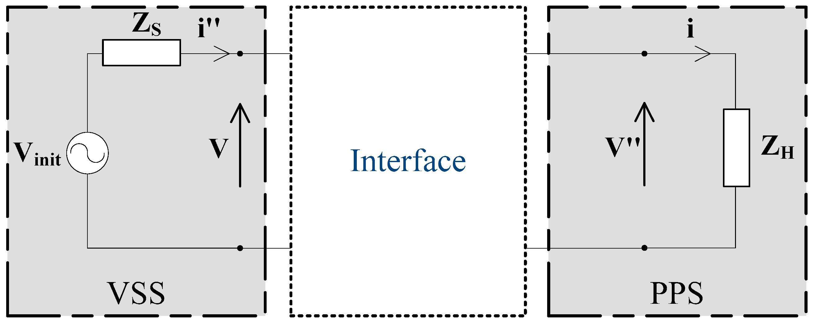
In general, a PHIL system architecture can be illustrated as a Thévenin equivalent, as depicted in Figure 1.

The VSS, represented by the voltage source V₀ and the internal simulation impedance Z_S, is used to run power system simulations mainly for power system stability studies.

The PPS, represented by the voltage or power source V₂, the measurement i₂, and the hardware impedance Z_H, contains a power amplifier, the hardware-under-test (HUT), and the measurement probes.

A PHIL system needs an interface to pass voltage or current from the VSS to the PPS and feed the dynamic behavior measured from the PPS as current and/or voltage flow back to the VSS.

The use of a power amplifier, as well as of probes, is essential for PHIL systems, but they influence the system dynamics and can introduce disturbances into the system [6,7]. Several algorithms were proposed in the last decade to ensure a stable operation of such a testing setup; however, the use of damping or filtering methods to ensure safe and stable experimental conditions influences the accuracy of the dynamic PHIL setup behavior. Finally, a compromise has to be found between more realistic test cases and larger stable operational ranges.

In the following, a comparison of the stable operational ranges of several IA and how to investigate them is presented.

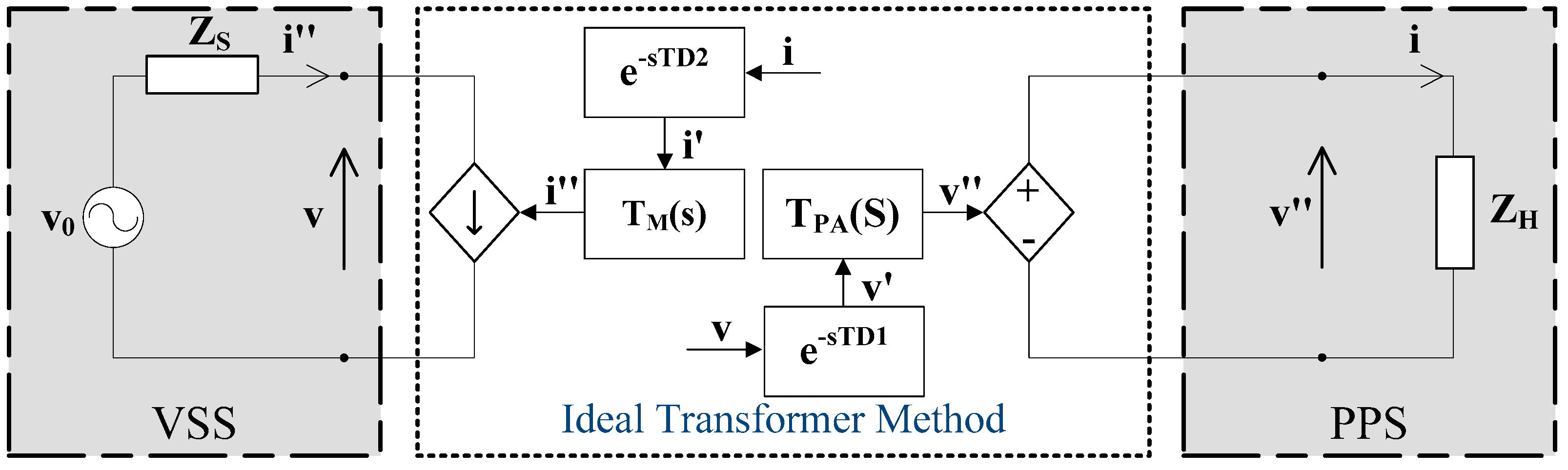
2.1. Ideal Transformer Method

The Ideal Transformer Method (ITM) presents the most general and straightforward method for linking the VSS with the PPS [5]. Its scheme is depicted in Figure 2 and can be described with the following open loop transfer function by Equation (1):

$$-{\mathrm{F}}_0\left(\mathrm{s}\right)={\mathrm{e}}^{-{\mathrm{sT}}_{\mathrm{D}}}\cdot {\mathrm{T}}_{\mathrm{PA}}\left(\mathrm{s}\right)\cdot {\mathrm{T}}_{\mathrm{M}}\left(\mathrm{s}\right)\cdot {\mathrm{Z}}_{\mathrm{S}}\left(\mathrm{s}\right)/{\mathrm{Z}}_{\mathrm{H}}\left(\mathrm{s}\right)$$

(1)

where T_D is the total time delay produced by the measurement probe T_D2 and the power amplifier T_D1, and T_PA and T_M represent the dynamic behavior of the power amplifier and the measurement probe, respectively.

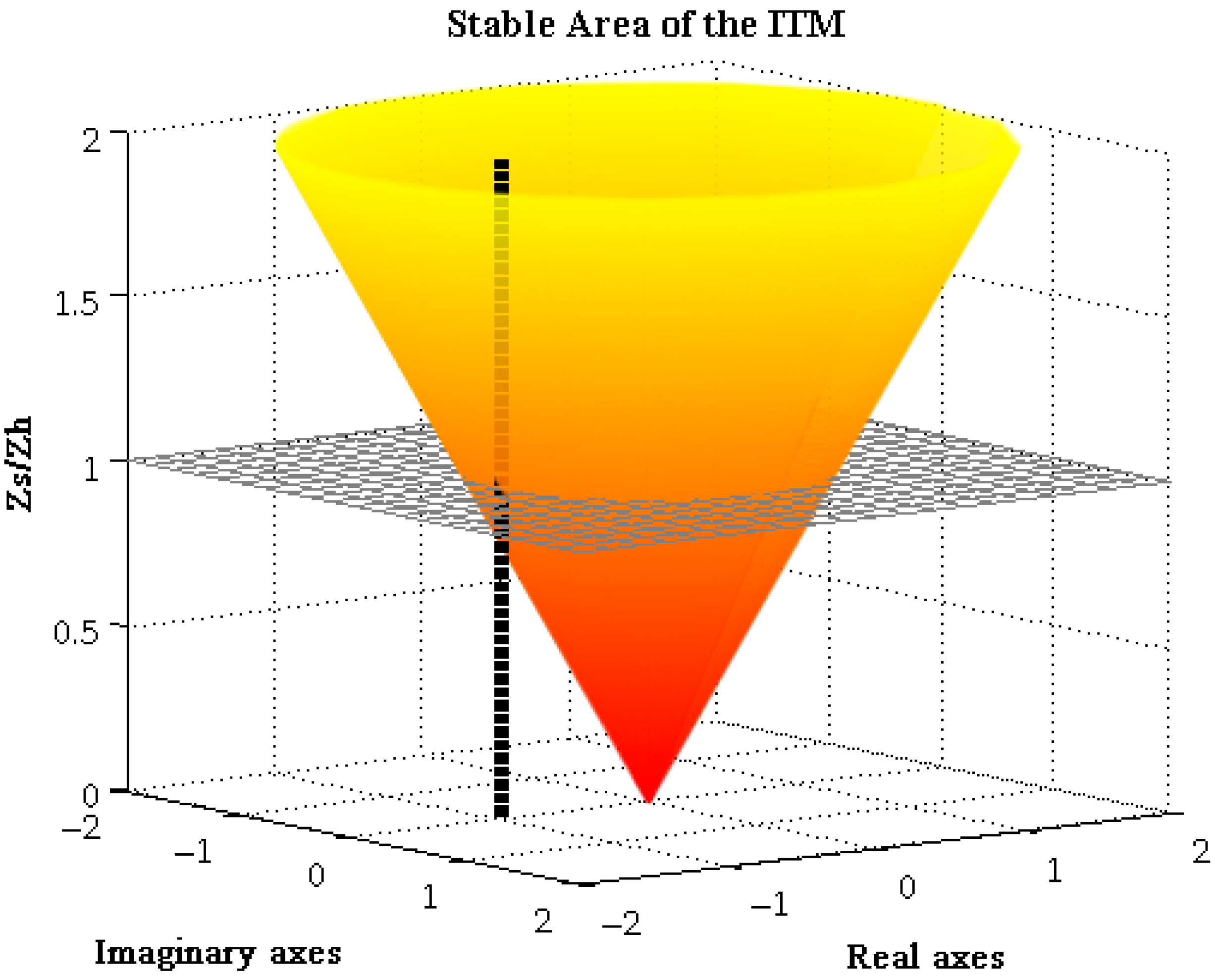
The ratio between the simulated impedance Z_S and hardware impedance Z_H is critical for the stable operational range of PHIL experiments, since its values will be changing during the test. Therefore, Nyquist calculations of the stable operational range of the ITM were made by using several impedance ratios.

Figure 3 shows the stable range of the ITM; everything that is below the added surface at the impedance ratio 1 will be a stable system. The intersection at Z_S/Z_H = 1 depicts the range until the system behaves in stable conditions. Above this, the system will not be stable according to the Nyquist criteria.

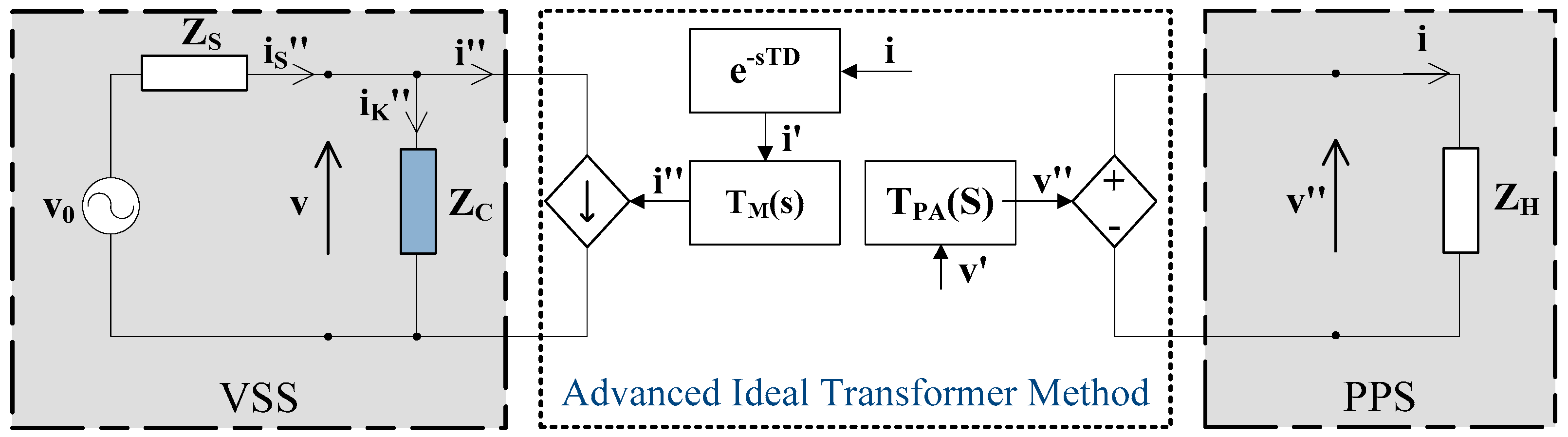
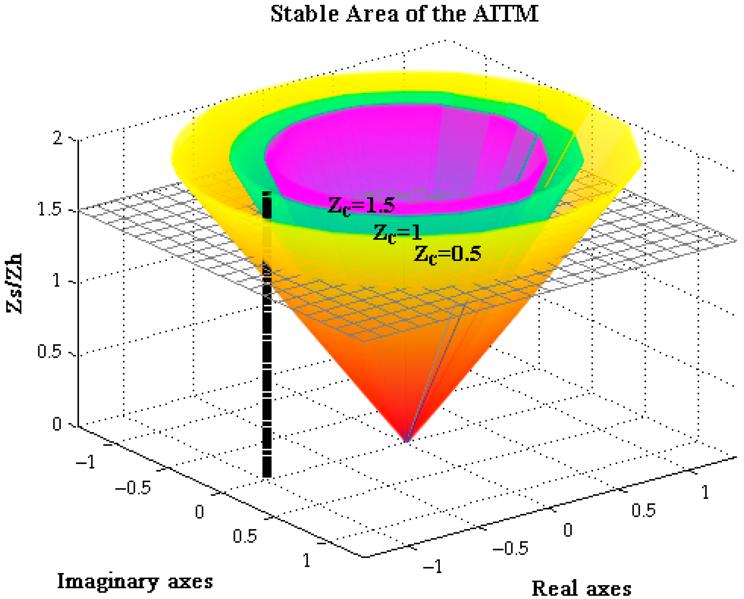
2.2. Advanced Ideal Transformer Method

To optimize the stable ranges of the ITM [8], an improvement of the method to an Advanced Ideal Transformer Method (AITM) is proposed by adding an extra compensation impedance Z_C in the VSS, as shown in Figure 4. The mathematical explanation of the AITM is given by Equation (2). Note that for the AITM, Z_C needs to be greater than 0 to avoid short-circuit conditions of the injecting current source given the “i′′.

$$-{\mathrm{F}}_0\left(\mathrm{s}\right)=\mathrm{e}^\left(-{\mathrm{sT}}_{\mathrm{D}}\right)\cdot {\mathrm{T}}_{\mathrm{LV}}\left(\mathrm{s}\right)\cdot {\mathrm{T}}_{\mathrm{M}}\left(\mathrm{s}\right)\cdot {\mathrm{Z}}_{\mathrm{S}}\left(\mathrm{s}\right)/\left({\mathrm{Z}}_{\mathrm{C}}\left(\mathrm{s}\right)+{\mathrm{Z}}_{\mathrm{H}}\left(\mathrm{s}\right)\right)$$

(2)

Figure 5 shows the stable ranges of the AITM for different compensation impedances. It can be seen that only for Z_C of 0.5 Ω will the system go into an unstable state, where the ratio of Z_S/Z_H is over 1.5 (red-yellow surface).

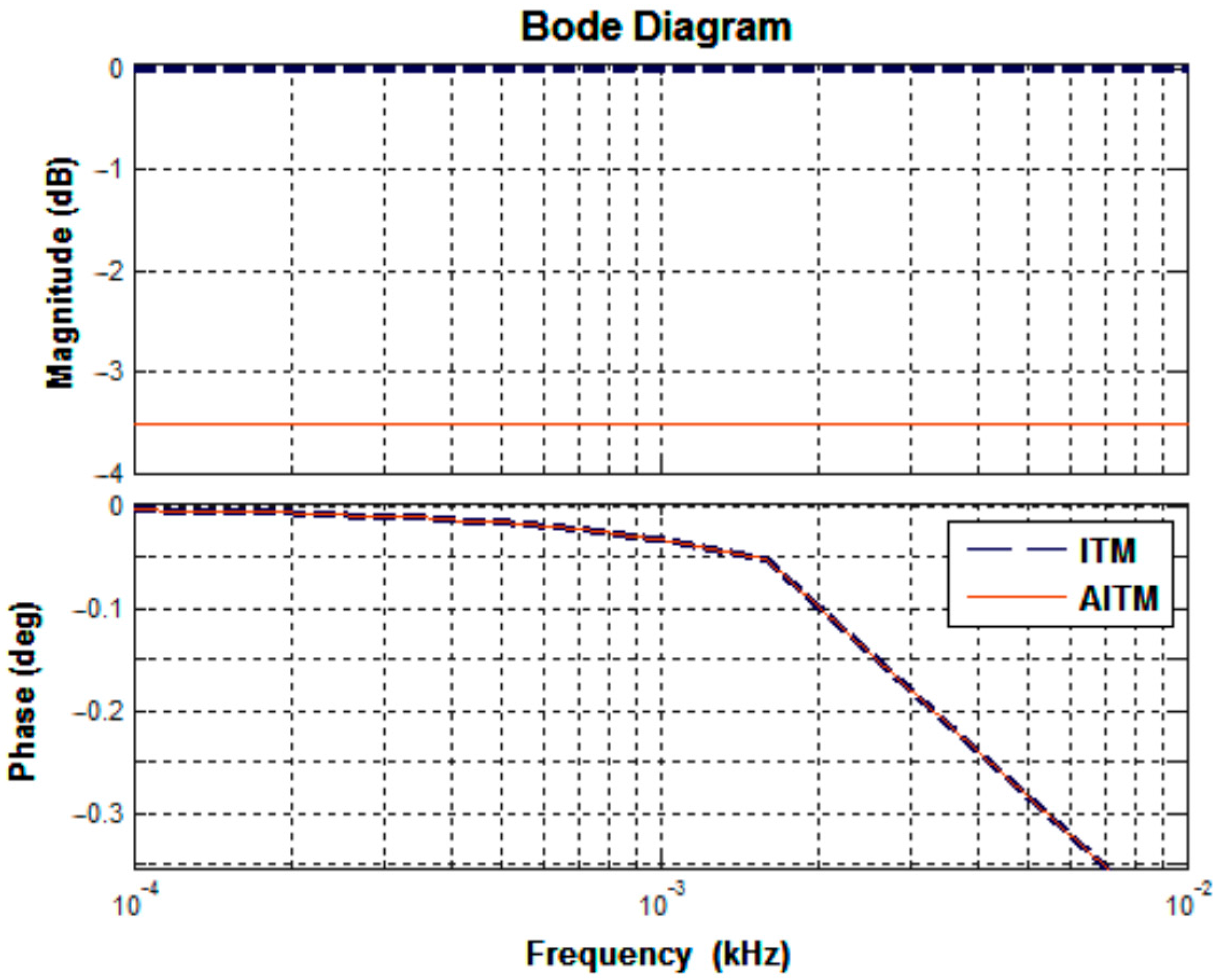
Nonetheless, adding additional components to the system (in software and hardware) can affect the accuracy of the results. Therefore, Z_C has to be as small as possible. This is shown below in the Bode diagram (Figure 6), where the ITM is compared to the AITM with a resistance of exemplary R_C = 0.5 Ω. By inserting a resistance, the magnitude of the system will be affected.

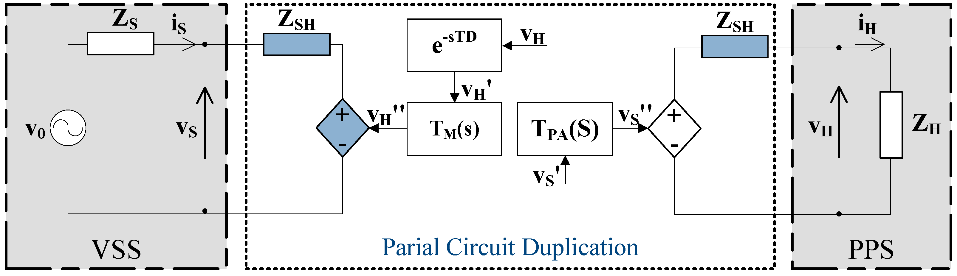
2.3. Partial Circuit Duplication

The method of the Partial Circuit Duplication (PCD) is presented in [9,10], and consists of additional coupling impedances Z_SH in the VSS and PPS (Figure 7). This method can be expressed as Equation (3). Note that the influence of the power amplifier and the measurement probe is omitted in Equation (3).

$$-{\mathrm{F}}_0\left(\mathrm{s}\right)\approx {\mathrm{Z}}_{\mathrm{S}}\left(\mathrm{s}\right)\cdot {\mathrm{Z}}_{\mathrm{H}}\left(\mathrm{s}\right)/\left(\left({\mathrm{Z}}_{\mathrm{S}}\left(\mathrm{s}\right)+{\mathrm{Z}}_{\mathrm{SH}}\left(\mathrm{s}\right)\right)\cdot \left({\mathrm{Z}}_{\mathrm{H}}\left(\mathrm{s}\right)+{\mathrm{Z}}_{\mathrm{SH}}\left(\mathrm{s}\right)\right)\right)$$

(3)

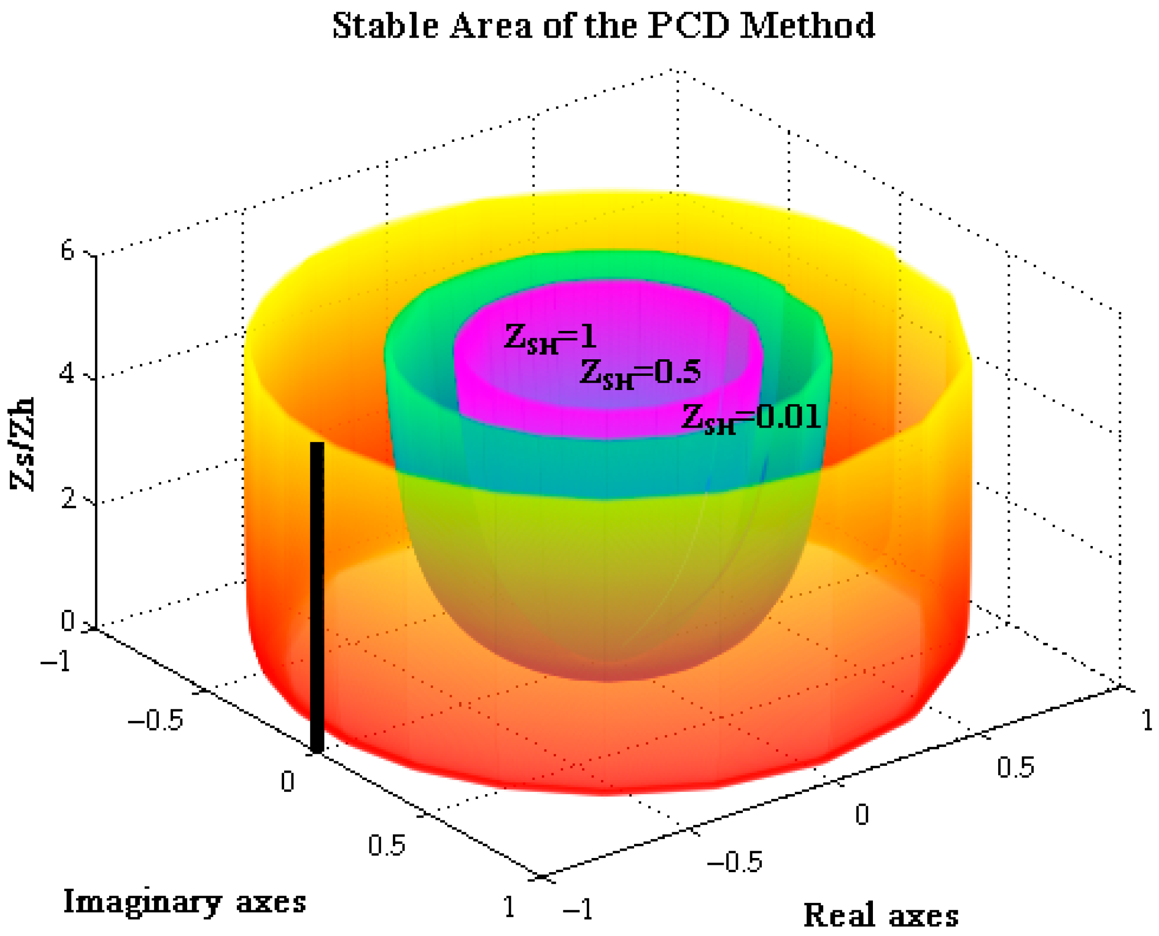
Figure 8 shows that even for small values of the coupling impedance Z_SH, the system will still operate in a stable condition. However, adding additional impedances in the VSS and the PPS means also a higher influence on the PHIL results due to the power consumption of the added components.

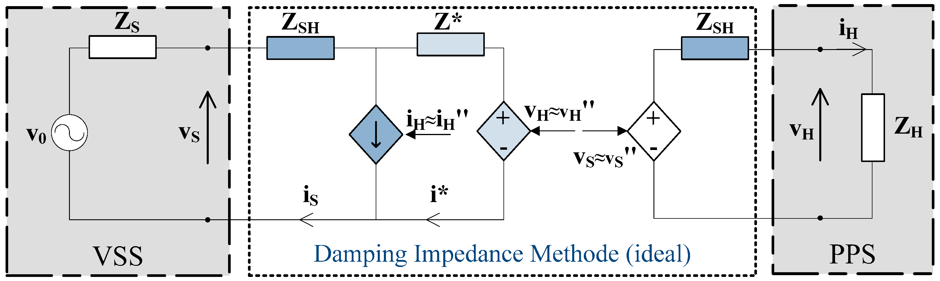
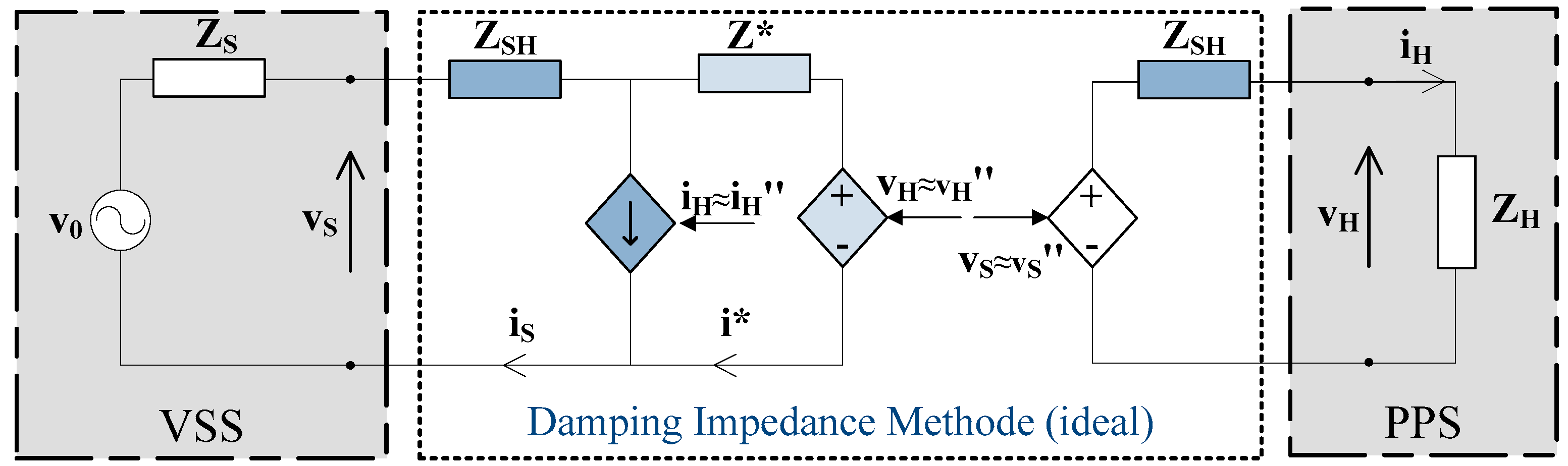
2.4. Damping Impedance Method

The Damping Impedance Method (DIM) combines the methods of the ITM and the PCD [5,11,12]. Its scheme is presented in Figure 9 and Equation (4) describe its dynamics. The DIM consists of an additional damping impedance Z* and will ensure absolute stability when Z* matches Z_H. Note that the influence of the power amplifier and the measurement probe are omitted.

$$-{\mathrm{F}}_0\left(\mathrm{s}\right)\approx {\mathrm{Z}}_{\mathrm{S}}\left(\mathrm{s}\right)\cdot \left({\mathrm{Z}}_{\mathrm{H}}\left(\mathrm{s}\right)-{\mathrm{Z}}^{*}\left(\mathrm{s}\right)\right)/\left(\left({\mathrm{Z}}_{\mathrm{H}}\left(\mathrm{s}\right)+{\mathrm{Z}}_{\mathrm{SH}}\left(\mathrm{s}\right)\right)\left({\mathrm{Z}}_{\mathrm{S}}\left(\mathrm{s}\right)+{\mathrm{Z}}_{\mathrm{SH}}\left(\mathrm{s}\right)+{\mathrm{Z}}^{*}\left(\mathrm{s}\right)\right)\right)$$

(4)

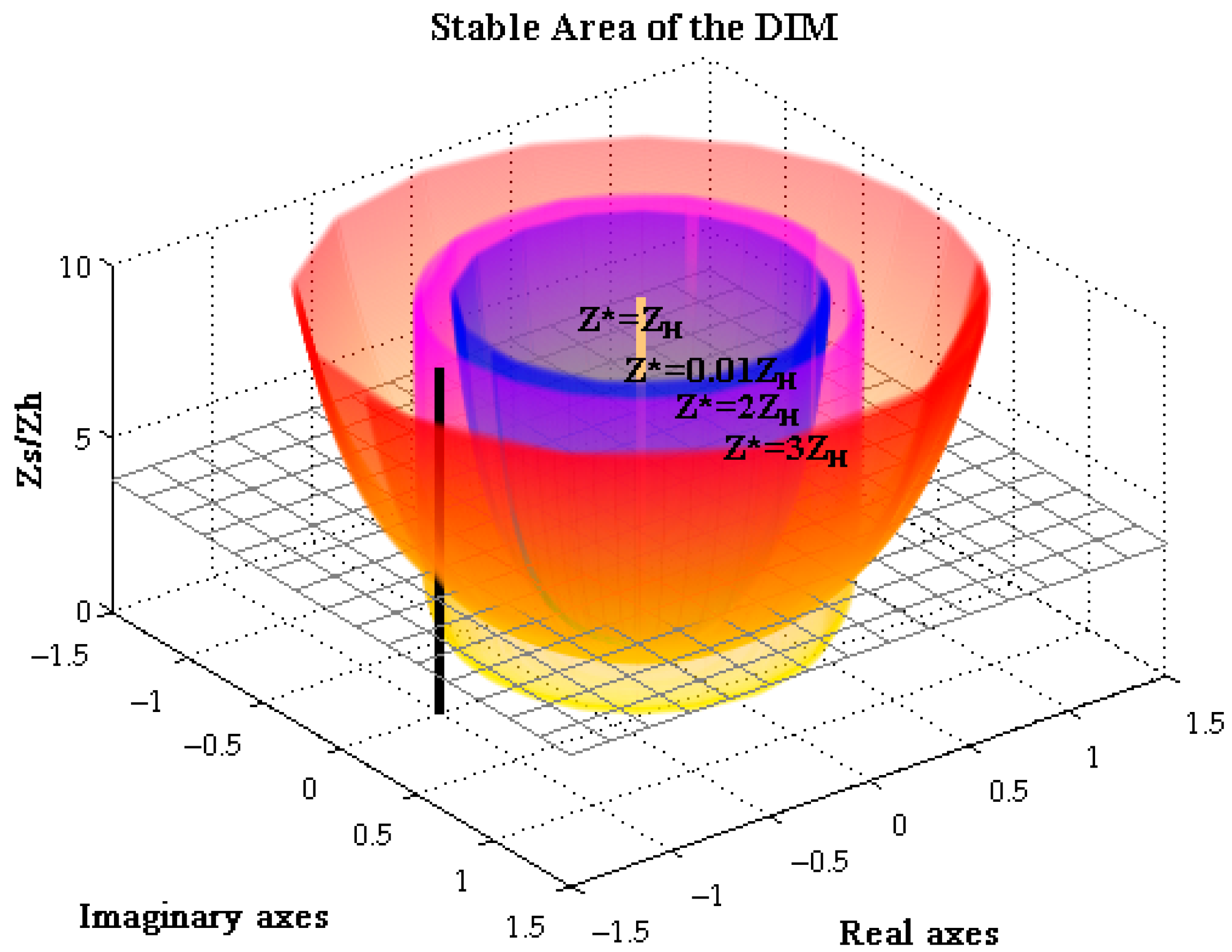
Compared to the calculations in the sections above, Figure 10 presents a wider stable operational range than any other method. For the case of Z* = Z_H there is no increase of stable conditions, only for Z* >> Z_H or Z* << Z_H can the system be unstable.

To ensure an absolute stable case during the experiment, the damping impedance should be adapted during the test to match Z_H in any case [12,13].

The DIM needs high implementation efforts and costs for the additional hardware impedance Z_SH.

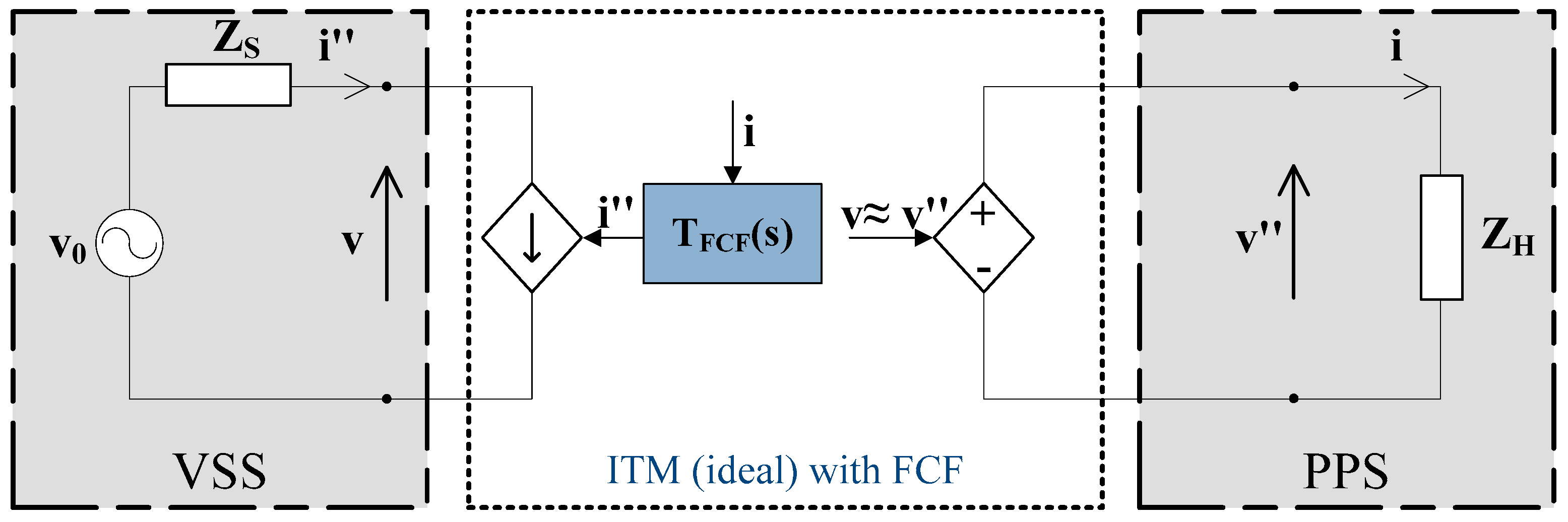
2.5. IA Extendible Feedback Current Filter

A Feedback Current Filter (FCF) can be used to extend the stable operational ranges of the discussed IA [4]. The feedback current or voltage is filtered by a band pass or low pass filter to cut undesired harmonics and noise. Figure 11 shows an example of the ITM with additional FCF. The mathematical expression is given by Equation (5). Note that the influence of the power amplifier and the measurement probe are omitted in Figure 11.

$$-{\mathrm{F}}_0\left(\mathrm{s}\right)=\mathrm{e}^\left(-{\mathrm{sT}}_{\mathrm{D}}\right)\cdot {\mathrm{T}}_{\mathrm{LV}}\left(\mathrm{s}\right)\cdot {\mathrm{T}}_{\mathrm{M}}\left(\mathrm{s}\right)\cdot {\mathrm{T}}_{\mathrm{FCF}}\left(\mathrm{s}\right)\cdot {\mathrm{Z}}_{\mathrm{S}}\left(\mathrm{s}\right)/{\mathrm{Z}}_{\mathrm{H}}\left(\mathrm{s}\right)$$

(5)

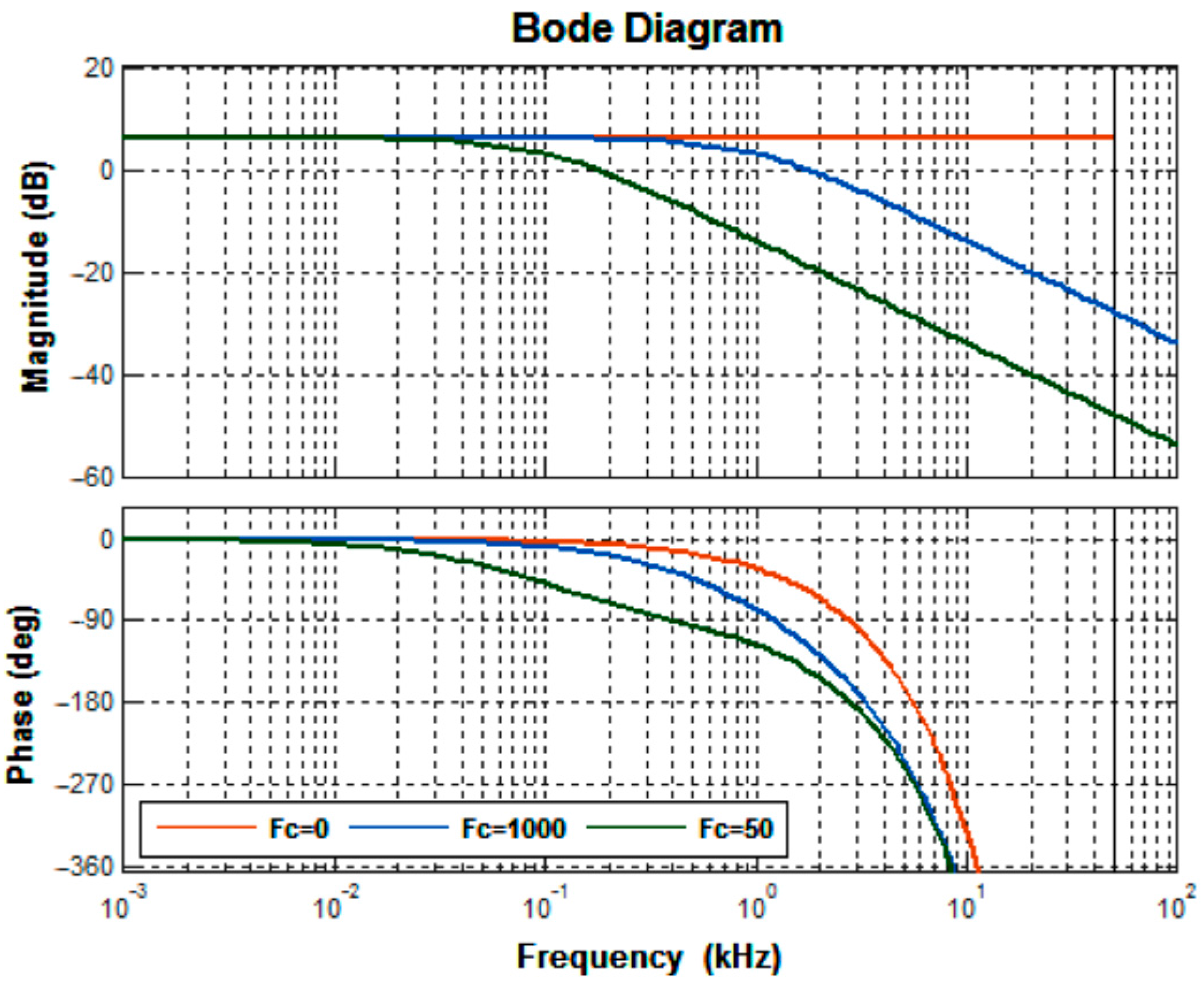
T_FCF represents the dynamic influence of the FCF in the system. For the use of a low pass filter with different cutting frequencies f_C, the following calculations were made.

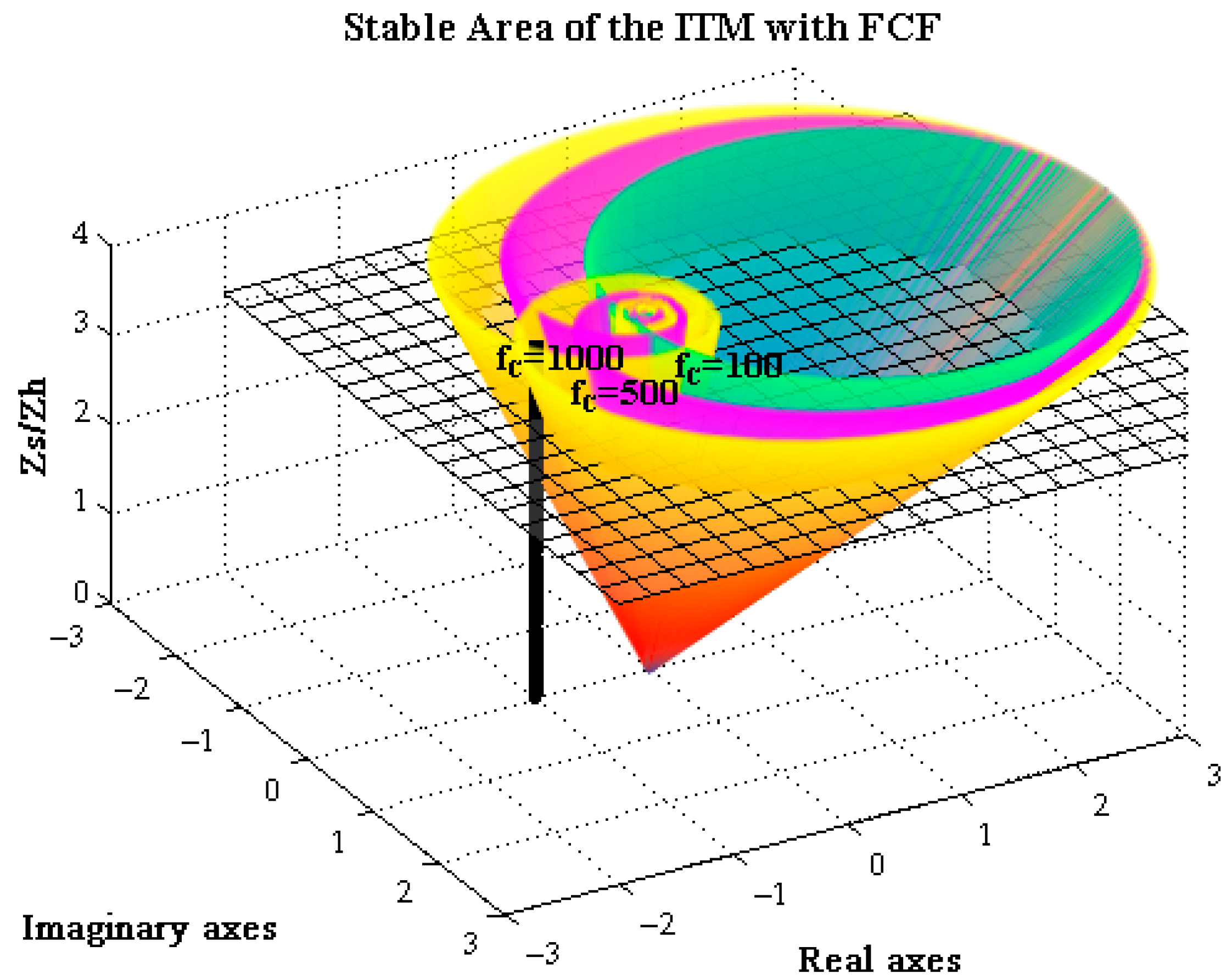
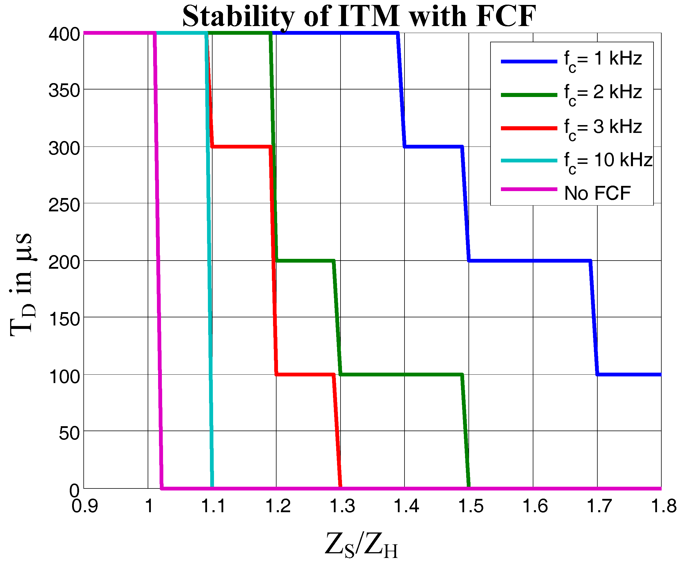
As Figure 12 depicts, the ITM can be improved by adding a FCF. Without an additional filter, the stable area of the ITM was trespassed at a ratio higher than 1. With a FCF of f_C = 1000 Hz, the ratio can be increased to 3.13. The advantage of the FCF is that every IA can be improved with it, but contrary to the increased operational range, the FCF can affect the accuracy of exchanged signals between the VSS and PPS depending on the chosen cut-off frequency f_C, as it can be seen in the loss of magnitude in Figure 13.

2.6. Summary

Table 1. Comparison of interface algorithms (IA).

Interface Algorithm	Mathematical Expression	Pro and Contra
Ideal Transformer Method	${\mathrm{Z}}_{\mathrm{S}}\left(\mathrm{s}\right)/{\mathrm{Z}}_{\mathrm{H}}\left(\mathrm{s}\right)$	+ best accuracy for PHIL + easy implementation − low stability
Advanced Ideal Transformer Method	${\mathrm{Z}}_{\mathrm{S}}\left(\mathrm{s}\right)/({\mathrm{Z}}_{\mathrm{C}}\left(\mathrm{s}\right)+{\mathrm{Z}}_{\mathrm{H}}\left(\mathrm{s}\right))$	+ high accuracy + easy implementation + good stability
Partial Circuit Duplication	${\mathrm{Z}}_{\mathrm{S}}\left(\mathrm{s}\right)\cdot {\mathrm{Z}}_{\mathrm{H}}\left(\mathrm{s}\right)/$ $\left(\left({\mathrm{Z}}_{\mathrm{S}}\left(\mathrm{s}\right)+{\mathrm{Z}}_{\mathrm{SH}}\left(\mathrm{s}\right)\right)\cdot \left({\mathrm{Z}}_{\mathrm{H}}\left(\mathrm{s}\right)+{\mathrm{Z}}_{\mathrm{SH}}\left(\mathrm{s}\right)\right)\right)$	+ extreme high stability − additional hardware required − low accuracy
Damping Impedance Method	${\mathrm{Z}}_{\mathrm{S}}\left(\mathrm{s}\right)\cdot \left({\mathrm{Z}}_{\mathrm{H}}\left(\mathrm{s}\right)-{\mathrm{Z}}^{*}\left(\mathrm{s}\right)\right)/$ $\left(\left({\mathrm{Z}}_{\mathrm{S}}\left(\mathrm{s}\right)+{\mathrm{Z}}_{\mathrm{SH}}\left(\mathrm{s}\right)\right)\left({\mathrm{Z}}_{\mathrm{H}}\left(\mathrm{s}\right)+{\mathrm{Z}}_{\mathrm{SH}}\left(\mathrm{s}\right)+{\mathrm{Z}}^{*}\left(\mathrm{s}\right)\right)\right)$	+ great stability + good accuracy − additional hardware required
Feedback Current Filter	${\mathrm{T}}_{\mathrm{FCF}}\left(\mathrm{s}\right)\cdot {\mathrm{Z}}_{\mathrm{S}}\left(\mathrm{s}\right)/{\mathrm{Z}}_{\mathrm{H}}\left(\mathrm{s}\right)$	+ Extendible feature for IA + easy implementation − accuracy depending on fC

summarizes the mathematical explanations and gives an overview of the advantages and issues of each presented IA.

3. Comparison of Power Amplifier with Power Hardware-in-the-Loop Systems

Contrary to Controller Hardware-in-the-Loop systems, PHIL Systems need additional voltage and power sinks or sources to adapt low-level signals from the Real-Time Simulator to the level of the HUT [6,14]. For carrying out PHIL experiments [4], the dynamic behavior of power amplifiers has to be considered, due to additional delays and internal filters that they introduce.

For upcoming investigations, two different kinds of amplifier are planned to be used to compare the behavior of PHIL systems: the switching amplifier and linear amplifier.

3.1. Switching Amplifier

Switching amplifiers are alternating/direct current converters and consist of a rectifier and an inverter. The advantages of the switching amplifiers are their efficiency in lower power ranges, but they can be built up to megawatt-ranges in compact and cost-reduced ways. Because of their internal pulsing of the output voltage coming from switching components, they are susceptible to harmonics and flickers. Furthermore, the reaction of the switching compared to linear amplifiers are slower [6] (see swell rate in

Table 2. Parameters of the amplifiers and measurement probes.

System Parameter	Linear Amplifier	Switching Amplifier	Current Probe	Voltage Probe
Model	S & S PAS 90000	Ametek RS 270	LEM HTA 1000	LEM CV 3–100 V
Power	3 × 30 kVA	3 × 3 × 30 kVA	1000 A	1000 V
Bandwidth	DC … 5 kHz	DC … 2 kHz	DC … 50 kHz	DC … 800 kHz
Swell rate	>52 V/µs	>0.5 V/µs	>50 A/µs	0.4 µs to 90% VN

).

3.2. Linear Amplifier

The linear amplifier provides, besides the functionalities of the switching amplifier, the possibility to operate it in a linear range, which implies faster response and adaptation of the low-level signals from the VSS; on the contrary, disturbances and transient effects are also amplified which switching amplifiers may damp. The disadvantage of the linear amplifier is the limited operational range compared to switching amplifiers. Therefore, the costs and dimensions are higher for the same power levels [15].

3.3. Comparison of Power Amplifiers

Table 2 provides the parameter of the used amplifiers.

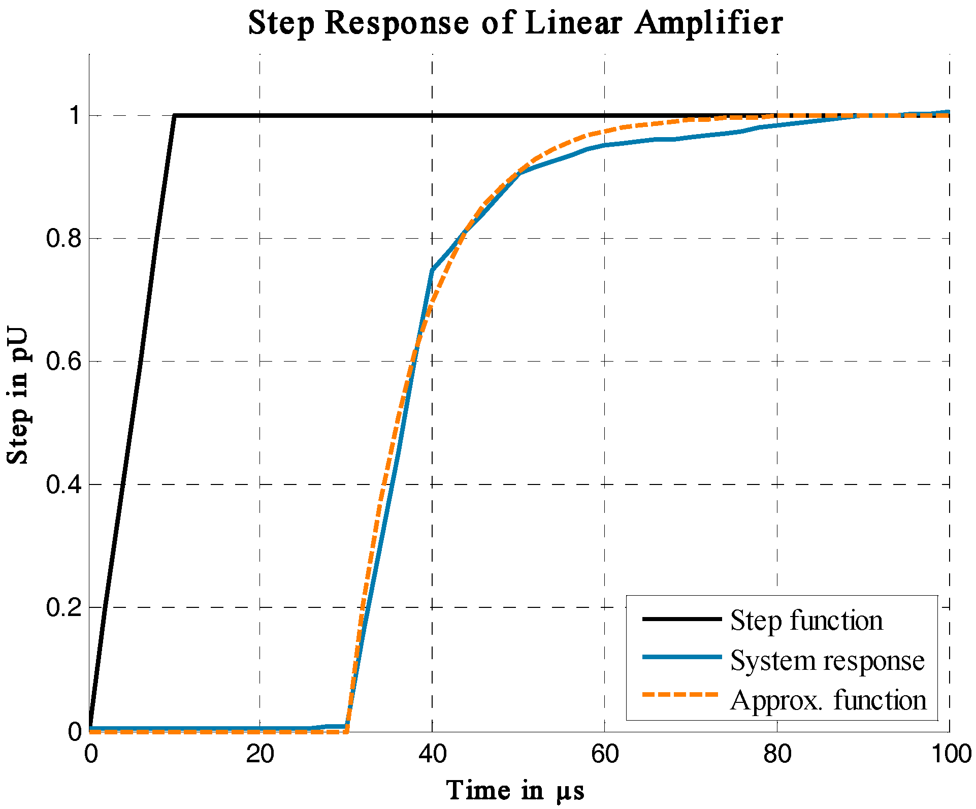
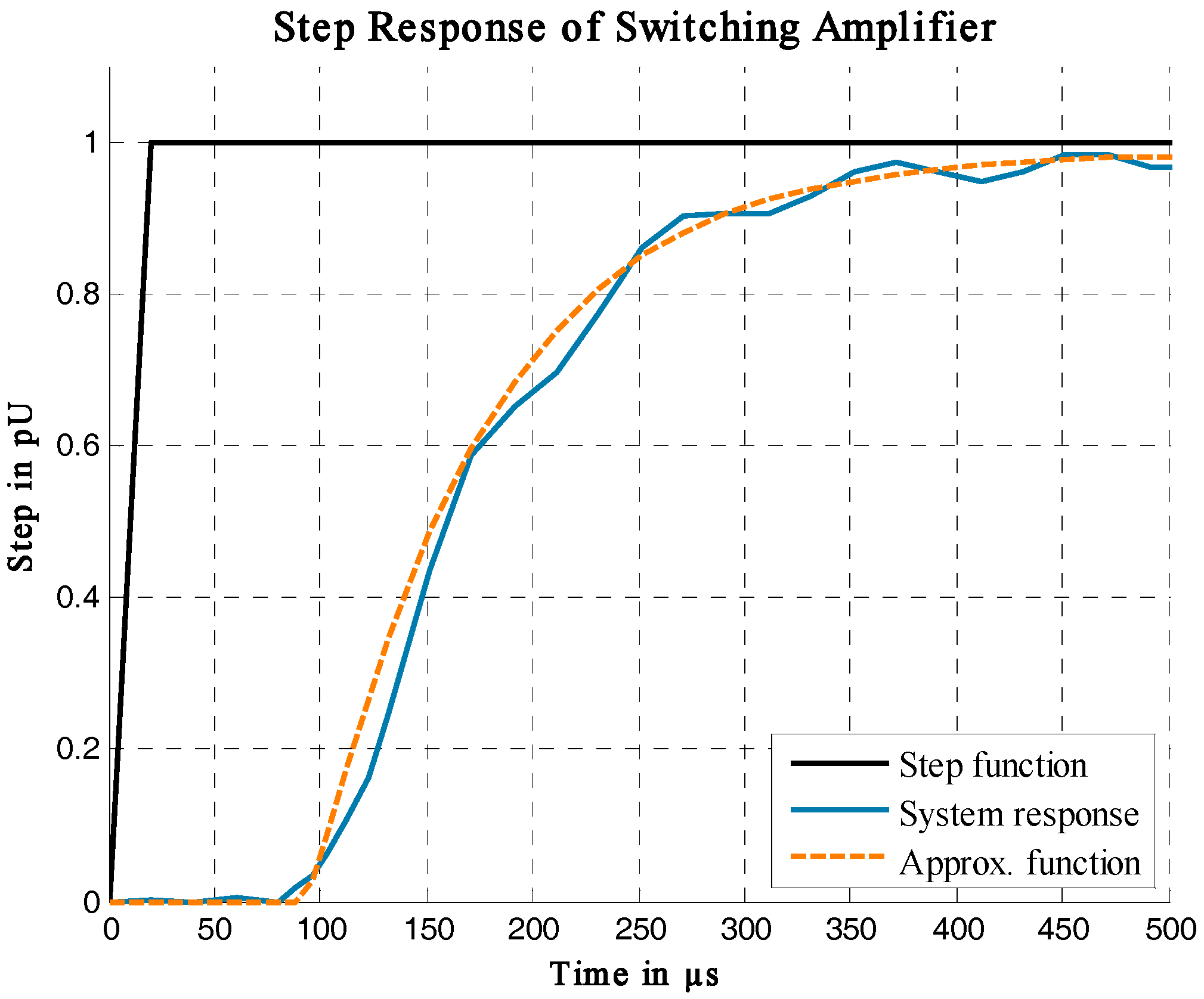
To analyze dynamic behaviors of power amplifiers, a step signal can be input to investigate their response and related characteristics. The step response and mathematical expression of the behavior of the used amplifiers are given in Figure 14 and Figure 15, as well as in Equation (6) for the switching amplifier and in Equation (7) for the linear amplifier.

$$\begin{gathered} -{\mathrm{F}}_0{\left(\mathrm{s}\right)}_{\mathrm{swichted}}={\mathrm{e}}^{-90\mathsf{\mu }\mathrm{s}}\cdot \left(-5849{\mathrm{s}}^2+2.2\times {10}^9\mathrm{s}+2.2\times {10}^{12}\right) \\ / \left({\mathrm{s}}^3+181\times {10}^3{\mathrm{s}}^2+2.5\times {10}^9\mathrm{s}+2.2\times {10}^{12}\right) \end{gathered}$$

(6)

$$-{\mathrm{F}}_0{\left(\mathrm{s}\right)}_{\mathrm{linear}}={\mathrm{e}}^{-30\mathsf{\mu }\mathrm{s}}\times 5.5\times {10}^{12}/\left({\mathrm{s}}^2+12\times {10}^9\mathrm{s}+1.4\times {10}^{12}\right)$$

(7)

The above diagrams (Figure 16) show that the linear amplifier is three times faster than the switching amplifier and has a smoother rise of the signal.

According to the step response test, the system with a linear amplifier delays the response with ${\mathrm{T}}_{\mathrm{D},\mathrm{linear}}=30$ µs and the switched amplifier with ${\mathrm{T}}_{\mathrm{D},\mathrm{switched}}=90$ µs. Both determined delays, including delays of input and output cards of the simulator, as well as delays generated by the measurement probes.

4. Preliminary Simulations of Power Hardware-in-the-Loop Systems

For a preliminary assessment of the possible operation ranges of PHIL experiments, the PHIL system was studied in pure simulation first. Therefore, the tested power system model, simplified as Thévenin circuit is connected to a chosen IA with an impedance model of the PPS as well as the power amplifiers’ dynamics analyzed in the previous section.

Figure 17 depicts the simulations model, where several IA are added to verify their operational ranges. During the simulation, the PPS was connected at 0.2 s to the VSS. Depending on the IA and the ratio of Z_S and Z_H, the simulation will be stable or not. Section 4.4 summarizes the conclusion of the investigated simulations.

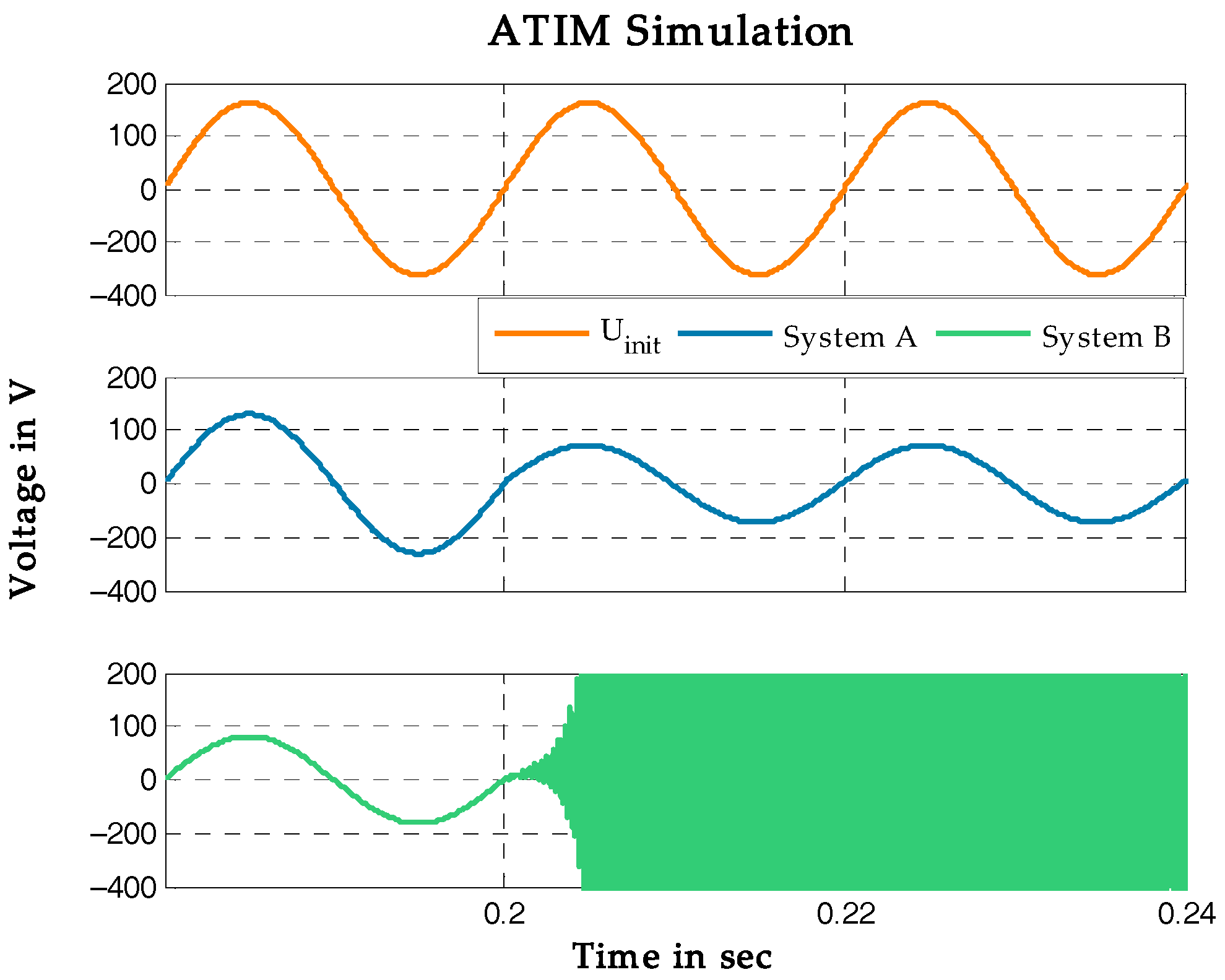
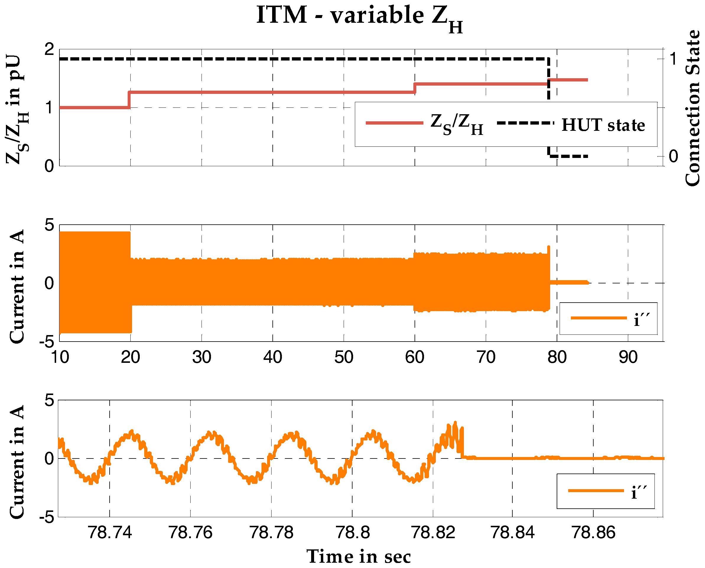
4.1. Simulation of the Ideal Transformer Method

Table 3. Parameters of ITM simulation.

ITM	System A	System B
VSS impedance ${\mathrm{R}}_{\mathrm{S}}$	1 Ω	2 Ω
PPS impedance ${\mathrm{R}}_{\mathrm{H}}$	1 Ω	1 Ω
Transfer function	${\mathrm{e}}^{-{\mathrm{T}}_{\mathrm{D}}}\cdot {\mathrm{T}}_{\mathrm{System}}\cdot {\mathrm{Z}}_{\mathrm{S}}/{\mathrm{Z}}_{\mathrm{H}}$
Result	Stable	Unstable

lists the used parameter for the preliminary ITM simulation studies. Figure 18 shows the results.

4.2. Simulation of the Advanced Ideal Transformer Method

Table 4. Parameters of AITM simulation.

AITM	System A	System B
VSS impedance ${\mathrm{R}}_{\mathrm{S}}$	3 Ω	4 Ω
PPS impedance ${\mathrm{R}}_{\mathrm{H}}$	1 Ω	1 Ω
Coupling imped. RSH	3.5 Ω	3.5 Ω
Transfer function	${\mathrm{e}}^{-{\mathrm{T}}_{\mathrm{D}}}\cdot {\mathrm{T}}_{\mathrm{System}}\cdot {\mathrm{Z}}_{\mathrm{S}}/({\mathrm{Z}}_{\mathrm{K}}+{\mathrm{Z}}_{\mathrm{H}})$
Result	Stable	Unstable

lists the used parameter for the preliminary AITM simulation studies. Figure 19 shows the results.

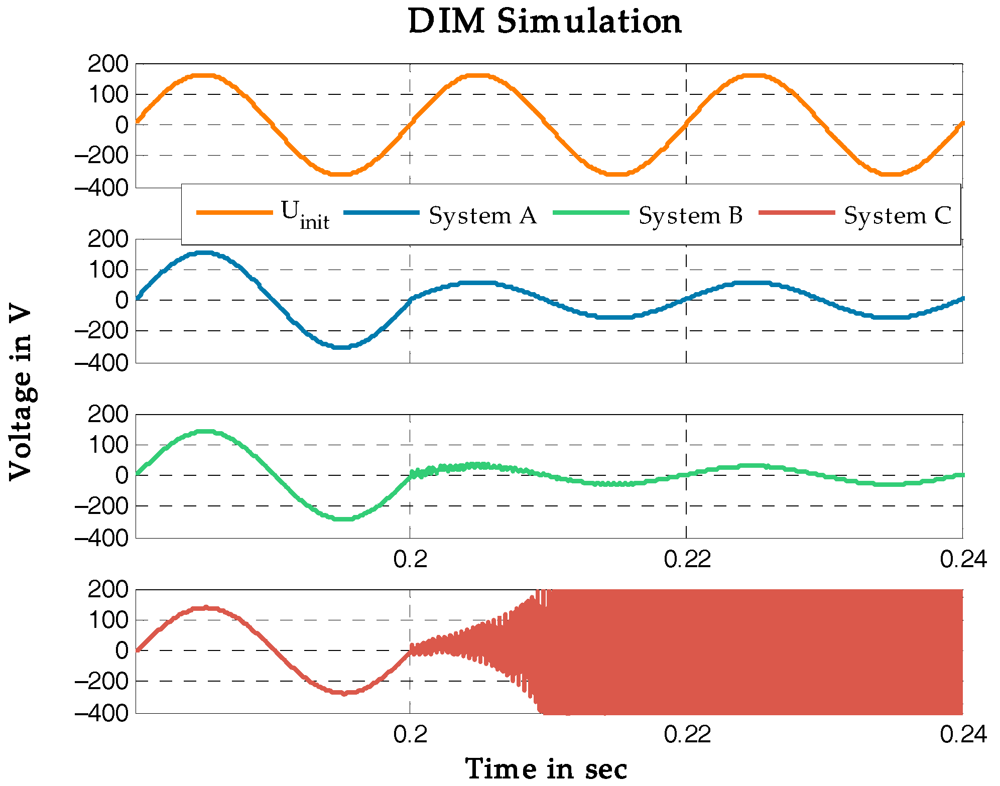
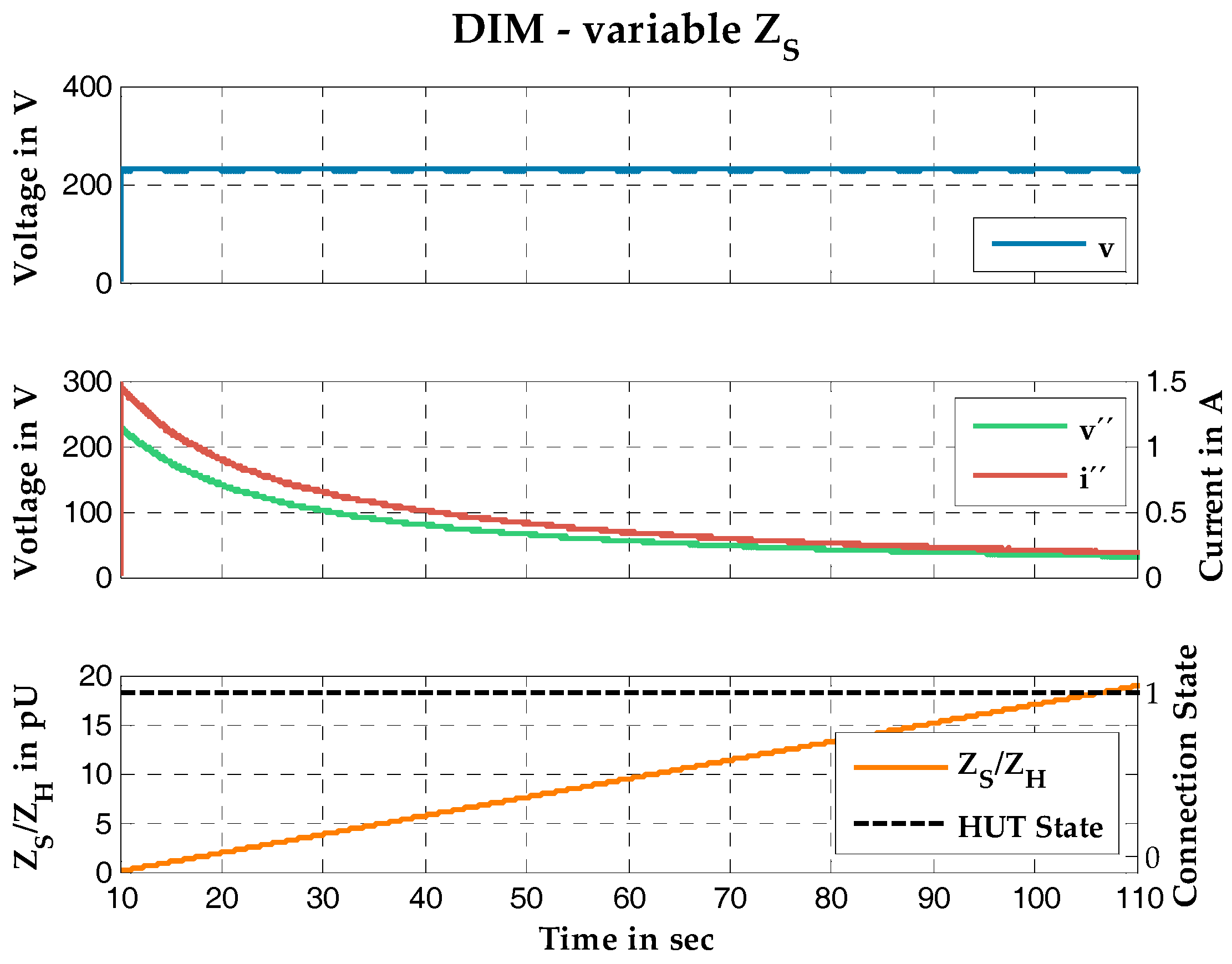
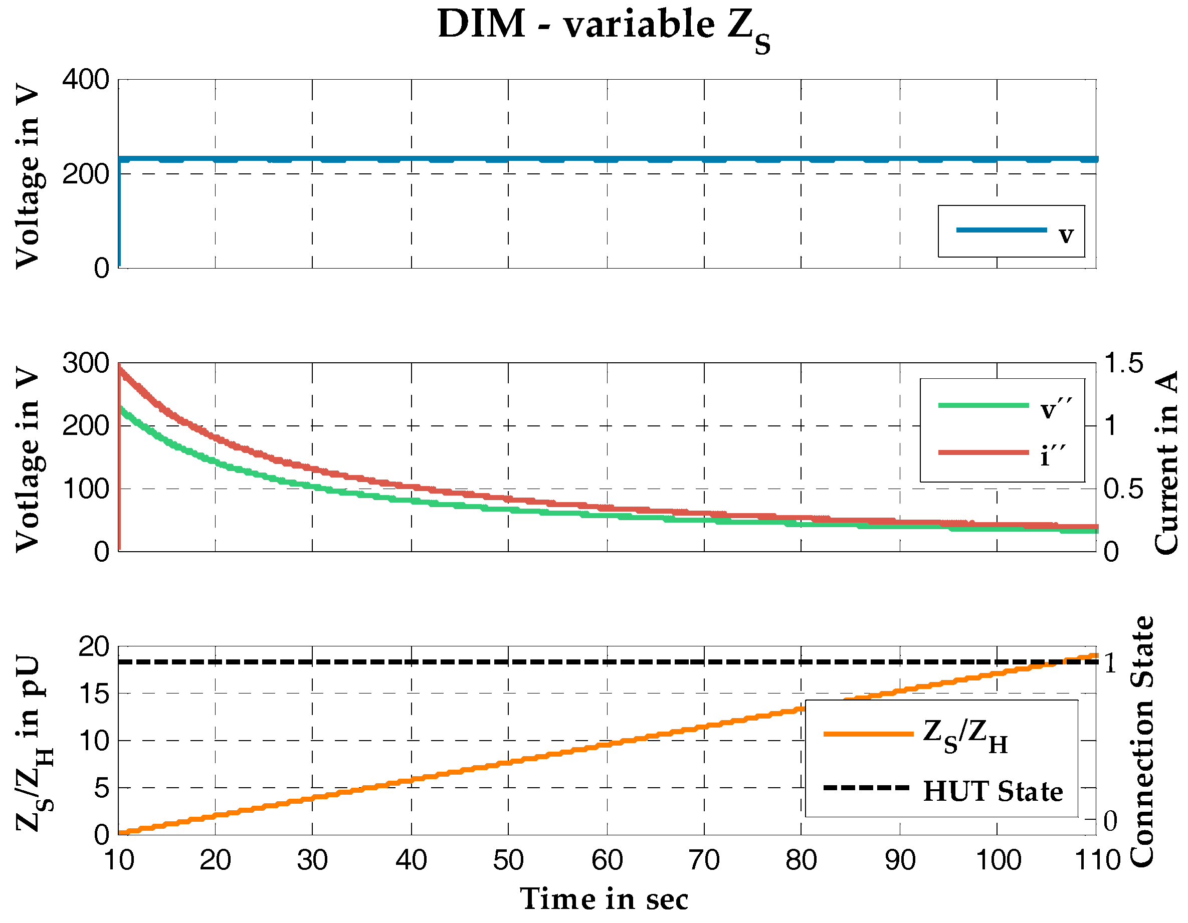
4.3. Simulation of the Damping Impedance Method

Table 5. Parameters of DIM simulation.

DIM	System A	System B	System C
Virtual impedance ${\mathrm{R}}_{\mathrm{S}}$	2 Ω	5 Ω	6 Ω
Coupling impedance ${\mathrm{R}}_{\mathrm{SH}}$	0.1 Ω	0.1 Ω	0.1 Ω
Damping impedance ${\mathrm{R}}^{*}$	3 Ω	3 Ω	3 Ω
Hardware impedance ${\mathrm{R}}_{\mathrm{H}}$	1 Ω	1 Ω	1 Ω
Transfer function	${\mathrm{e}}^{-{\mathrm{T}}_{\mathrm{D}}}\cdot {\mathrm{T}}_{\mathrm{System}}\cdot {\mathrm{Z}}_{\mathrm{S}}\left(\mathrm{s}\right)\left({\mathrm{Z}}_{\mathrm{H}}\left(\mathrm{s}\right)-{\mathrm{Z}}^{*}\left(\mathrm{s}\right)\right)/\left(\left({\mathrm{Z}}_{\mathrm{S}}\left(\mathrm{s}\right)+{\mathrm{Z}}_{\mathrm{SH}}\left(\mathrm{s}\right)\right)\left({\mathrm{Z}}_{\mathrm{H}}\left(\mathrm{s}\right)+{\mathrm{Z}}_{\mathrm{SH}}\left(\mathrm{s}\right)+{\mathrm{Z}}^{*}\left(\mathrm{s}\right)\right)\right)$
Simulation	Stable	Stable	Unstable

lists the used parameters for the preliminary DIM simulation studies. The damping impedance is designed with a higher value as the hardware impedance to simulate variable conditions. Figure 20 shows the results.

4.4. Conclusion of the IA Simulation Studies

Table 6. Stable cases of the IA simulations.

Stable Case	ITM	AITM	DIM
Virtual impedance ${\mathrm{R}}_{\mathrm{S}}$	1 Ω	5 Ω	6 Ω
Hardware impedance ${\mathrm{R}}_{\mathrm{H}}$	1 Ω	1 Ω	1 Ω
Ratio RS/RH	1	5	6

gives a comparison of the investigations’ results, at which impedance ratios of the simulation remain stable.

The differences between the calculated and simulations’ results are due to the added dynamics of the switching amplifier.

Table 6 shows which ratio of the impedances from VSS and PPS different IAs can handle. Furthermore, according to the impedance ratio, it can be stated that the DIM shows a higher stability than the AITM, which shows a higher stability than the ITM.

These investigations are not sufficient to set up PHIL experiments. In reality, several disturbances occur due to additional delays, amplifications errors, and electromagnetic compatibility (EMC) of wires and elements, which cannot be easily investigated by calculations or simulations. Therefore, real tests for stable operational ranges of the PHIL system itself have to be made to ensure a stable and safe experiment [11,16], and are shown in Section 5.

Nevertheless, the carried out preliminary studies provide a good overview concerning the choices of which IA can be used for different test cases.

5. Verification of IA in Real PHIL Systems

As mentioned above, running PHIL experiments can include additional disturbances which cannot be calculated or simulated. The following list will give a summary of what aspects have to be considered when setting up a PHIL system.

-

Reduce electromagnetic influences by using screened and short wires, especially for the low-level signals;

-

Reduce delays by using fast components and short connections;

-

All devices have to be in the same emergency circuit;

-

Integrate error detectors and protection devices (i.e., in the real-time simulator and power amplifier [17]);

-

Ensure the safety of the experiment setup, especially when using hardware like batteries and rotating machines.

The uses of power amplifiers with internal filters and resistances or inductances can increase the testing system stability due to the intrinsic behavior of the different components.

Two of the mentioned IAs (ITM and DIM) have been verified in a real PHIL system. The easy implementation and high accuracy makes the ITM the best choice for linear and not so complex cases. In addition, the DIM with its higher stable operational range and good accuracy is mostly used to investigate non-linear cases with a high range of different or variable operational points. Therefore, these two methods will be compared in the following by real lab-based experiments using different power amplifiers.

5.1. Testing the Ideal Transformer Method

5.1.1. Ideal Transformer Method with Linear Amplifier

The ITM has been tested while using a linear amplifier.

Table 7. Parameters of ITM experiment.

Parameter of ITM Experiment with Linear Amplifier
Voltage Uinit	230 V at 50 Hz
Virtual impedance RS	variable
Ratio of RS/RH	(0.9:0.1:1.8)
Physical impedance RH	105.90 Ω
FCF fC	(1:1:10) kHz
Additional delay TD	(0:25:400) µs
Method	ITM with FCF
Amplification system	Linear amplifier
Real-time simulator	OP5600 from OPAL-RT

gives the used parameter of the experiment. The results are shown in Figure 21.

Figure 21 depicts the stable areas of the used parameters. The integral of the several curves represents the range of the stable operation points.

5.1.2. Ideal Transformer Method with Switching Amplifier

The ITM has been tested while using a switching amplifier.

Table 8. Parameters of ITM experiment.

Parameters of ITM Test with Switching Amplifier
Voltage Uinit	230 V at 50 Hz
Virtual impedance RS	variable
Physical impedance RH	31.8 Ω
FCF fC	(1:1:10) kHz
Additional delay TD	(0; 50; 500; 1000) µs
Method	ITM with FCF
Amplification system	Switched amplifier
Real-time simulator	OP5600 from OPAL-RT

gives the used parameters of the experiment. The results are shown in Figure 22.

Figure 22 depicts the stable areas of the used parameters. It can be seen that there is no change about using a cut-off frequency higher than 2 kHz compared to no FCF. According to the bandwidth of the amplifier (see Table 2), the amplifier cuts off the frequency over 2 kHz by its internal filters. This means that a FCF with f_C ≥ 2 kHz won’t affect the results.

5.1.3. Conclusion of the ITM Experiments

The results of the ITM testing with different amplifiers lead to the conclusion that the internal filters of the switching amplifier have a positive effect on the system’s stability range. This implies that for the ITM with lower stability, a linear amplifier leads faster to unstable conditions. The use of additional FCF can stabilize the system and, by improving the method to the AITM, can increase the operational ranges of a PHIL experiment as well.

It can be seen in Figure 21 that a FCF over the bandwidth limit of 5 kHz (see Table 2) of the linear amplifier still affect the results. This comes from the used measurement probes in this case, as they had a low accuracy and created higher delays. Therefore, more accurate probes were used for the PHIL system experiments with the switching amplifier.

5.2. Testing the Damping Impedance Method

5.2.1. Damping Impedance Method with Linear Amplifier

The DIM has been tested while using a linear amplifier.

Table 9. Parameters of DIM experiment.

Paramteres of DIM Experiment with Linear Amplifier
Voltage Uinit	230 V at 50 Hz
Virtual impedance RS	variable
Damping impedance R*	variable
Coupling impedance RSH	variable
Physical impedance RH	105.90 Ω
Additional delay TD	(220) µs
Method	DIM
Amplification system	Linear amplifier
Real-time simulator	OP5600 from OPAL-RT

gives the used parameter of the experiment. The results are shown in Figure 23.

Figure 23 depicts the stable areas of the used parameters.

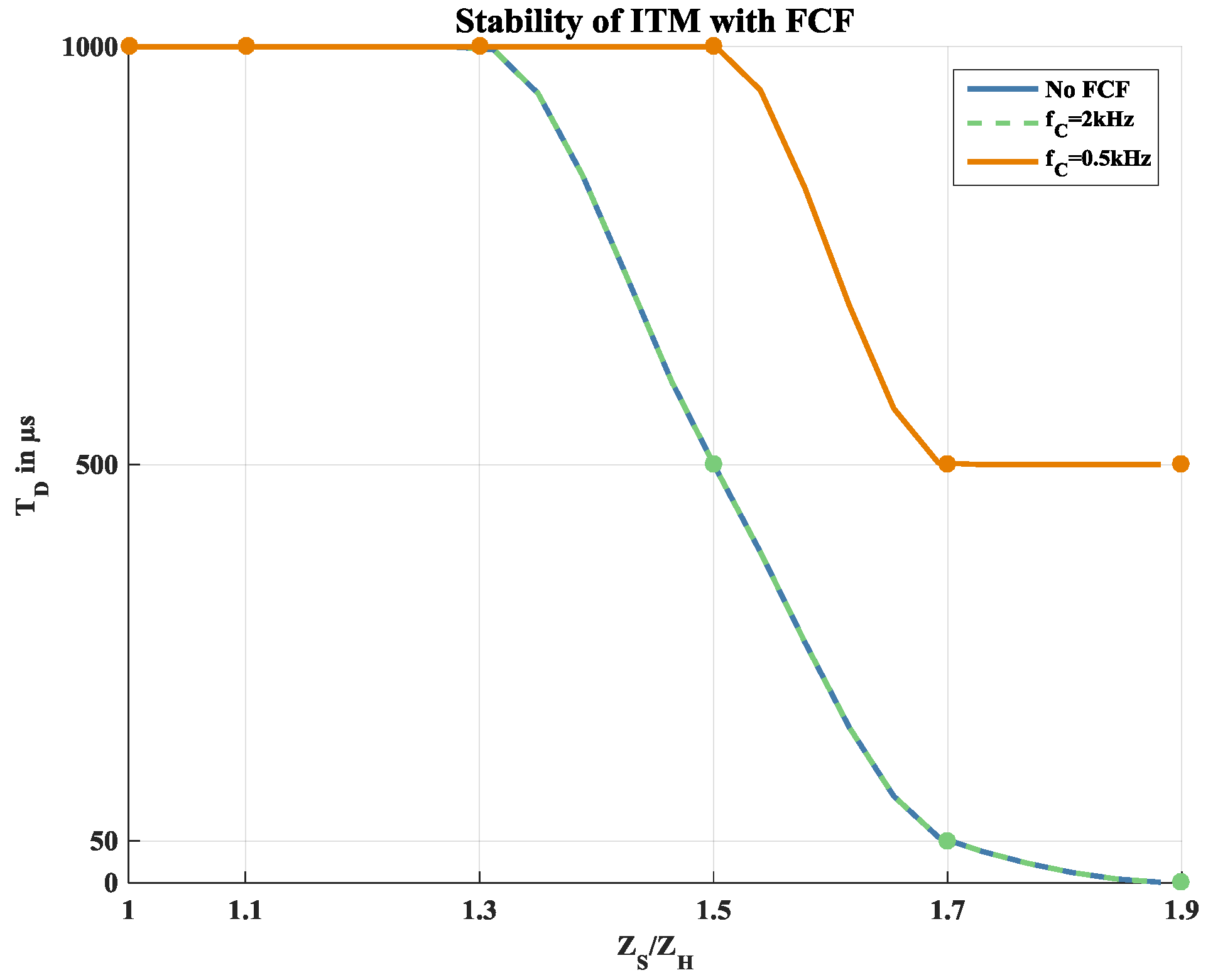
5.2.2. Damping Impedance Method with Switching Amplifier

The DIM has been tested while using a switching amplifier.

Table 10. Parameters of DIM experiment.

Parameters of DIM Experiment With Switching Amplifier
Voltage Uinit	230 V at 50 Hz
Virtual impedance RS	variable
Damping impedance R*	variable
Coupling impedance RSH	0.23 Ω
Physical impedance RH	31.8 Ω
Additional delay TD	variable
Amplification system	Switched amplifier
Real-time simulator	OP5600 from OPAL-RT

gives the used parameters of the experiment. The results are shown in Figure 24.

Figure 24 depicts the stable areas for different cases of the experiment.

5.2.3. Conclusion of the DIM Experiments

Using methods with additional stability functionality, like the tested DIM, results in a much higher operational range for the system. It is also seen that if the impedances between the VSS and PPS are matching, respectively Z_S/Z_H ≤ 1, the highest stability is given.

Furthermore, additional delays do not affect the DIM (Figure 24 dashed blue line) as they affect the ITM. Adding an extra FCF can increase the stability range of the DIM.

Moreover, it was shown that the DIM has a wider stable operational range than the ITM.

6. Experimental Investigation of ITM and DIM

The experimental studies serve as proof of concept for the undertaken analysis of the ITM and DIM in a laboratory setup by using ohmic load. For this purpose, the VSS or PPS changed continuously to test the limits of the stability of the entire system.

Table 11. Test cases of the ITM and DIM.

Test Case	1	2
Description	Review of the ITM interface with resistive physical load.	Review the DIM interface with resistive physical load.
Scenario	(a) Variation of virtual impedance (b) Variation of physical impedance	(a) Variation of virtual impedance (b) Variation of physical impedance

presents the performed test cases.

6.1. Test Case 1: ITM

In scenario (a), the virtual impedance is variable in the range of 0 < R_s < 1 kΩ. Due to laboratory setup limitation, the physical impedance was chosen with a constant value of R_H = 53 Ω during the entire test. A FCF set to f_G = 2 kHz was chosen. In both scenarios of test case 1, the ITM has been used.

In scenario (b), a constant value for the virtual impedance RS 100 = Ω was set and the physical impedance varies.

Figure 25 depicts the scheme of the performed experimental setup.

A shutdown of the HUT occurred for both scenarios (see Figure 26 and Figure 27), due to a detected overshoot of the selected 20% of total harmonic distortion (THD) threshold. Only stable operations of R_S/R_H < 1.5 could be achieved. This finding validates the stability analysis of the linear amplifier at f_G = 20 kHz presented in Section 5 (see Figure 21).

6.2. Test Case 2: DIM

Same investigation scenarios have been undertaken for the DIM as in test case 1. Due to laboratory setup limitation the value of the coupling impedance was selected with R_SH = 104.9 Ω.

Contrary to the performed studies of the ITM, the DIM experiment does not show any unstable operations during the entire experiment. It should be noted that the large coupling impedance has a great effect on the values, therefore it should be wisely chosen according to the envisaged investigations.

Figure 28 depicts the scheme of the performed experimental setup.

The experiments (shown in Figure 29 and Figure 30) confirm the conclusions of the analytical investigations performed for checking the stability limits of the ITM and DIM. It can be noted that the DIM has proven a wider range of stability under the same testing scenarios and conditions.

7. Conclusions

The paper presented an overview of interfaces for PHIL systems and compared the stable operational ranges of different interface algorithms, like the ITM, AITM, etc.

It has presented a way to investigate the functionality of different IA by using their mathematical equations, simulations—including physical component behaviors—and real laboratory experiments in Section 2.

According to the analyzed behavior of different IAs, the achieved results from the IA performance can be assessed.

Pure simulations including the characteristic of the PHIL system should be made to analyze which IA can be used (see Section 4).

It is important to investigate the capabilities of the PHIL system by performing preliminary stability tests (see Section 3). As shown in Section 5, good knowledge about the used components in a PHIL system is essential.

As a conclusion of the performed investigations, it can be stated that it is reasonable to start tests with high-accuracy IA and then, if necessary, gradually migrate towards IAs with wider operational ranges.

After investigating the combination of real-time simulations and power interfaces in a linear manner, as a next step to provide a generic stability description of PHIL systems, non-linear HUT is planned to be included in the initial studies of PHIL setups (e.g., inverters, active loads, etc.).