Optimal Dispatching of Active Distribution Networks Based on Load Equilibrium


1
State Key Laboratory of New Energy Power System, North China Electric Power University, Beijing 102206, China
2
Department of Electrical and Computer Engineering, Baylor University, Waco, TX 76798-7356, USA
*
Author to whom correspondence should be addressed.
Energies 2017, 10(12), 2003; https://doi.org/10.3390/en10122003
Submission received: 12 October 2017
/
Revised: 6 November 2017
/
Accepted: 22 November 2017
/
Published: 1 December 2017
(This article belongs to the Section F: Electrical Engineering)
Abstract
:This paper focuses on the optimal intraday scheduling of a distribution system that includes renewable energy (RE) generation, energy storage systems (ESSs), and thermostatically controlled loads (TCLs). This system also provides time-of-use pricing to customers. Unlike previous studies, this study attempts to examine how to optimize the allocation of electric energy and to improve the equilibrium of the load curve. Accordingly, we propose a concept of load equilibrium entropy to quantify the overall equilibrium of the load curve and reflect the allocation optimization of electric energy. Based on this entropy, we built a novel multi-objective optimal dispatching model to minimize the operational cost and maximize the load curve equilibrium. To aggregate TCLs into the optimization objective, we introduced the concept of a virtual power plant (VPP) and proposed a calculation method for VPP operating characteristics based on the equivalent thermal parameter model and the state-queue control method. The Particle Swarm Optimization algorithm was employed to solve the optimization problems. The simulation results illustrated that the proposed dispatching model can achieve cost reductions of system operations, peak load curtailment, and efficiency improvements, and also verified that the load equilibrium entropy can be used as a novel index of load characteristics.
1. Introduction
The rapid development of modern society has brought with it issues, including energy shortages and environmental pollution. To overcome these issues, it is crucial to exploit renewable energy (RE) [1,2] resources. In recent years, the installed capacities of RE have been rapidly increasing around the world. For example, in China, the generating capacities of wind power and photovoltaic (PV) power were 131 GW and 42 GW, respectively, by the end of 2015 [3]. Moreover, according to a recent report by the Energy Research Institute of the Chinese National Development and Reform Commission, both the RE electricity integration ratios of wind power and PV power are expected to reach approximately 30%, and their sum may rise to as much as 63% by 2050 [4,5]. However, the increased penetration of RE resources into distribution systems may lead to bidirectional power flow and bring abundant volatility and uncertainty, resulting in tremendous challenges to traditional distribution networks. To deal with these issues, traditional distribution networks are gradually evolving from a passive mode to an active mode. Hence, the concept of Active Distribution Networks (ADNs) [6,7,8,9] has been proposed. In the context of ADNs, distributed energy resources (DERs) (containing RE generators), controllable loads, and energy storage equipment can be actively adjusted using intelligent control techniques to attain specific operation objectives [10].
The extant research has been primarily focused on the control [11,12], protection [13,14], and dispatching [15,16,17,18] of ADNs. This study will investigate optimal ADN dispatching. Golshannavaz et al. [15] presented an optimal operational scheduling framework for intelligent distribution systems that are aimed at minimizing the day-ahead total operation costs to optimally control the active elements of distributed generations, the network, and demand response loads. In Ref. [16], the objective of the operation model was to maximize the social welfare in a real-time distribution energy market based on locational marginal prices. A new probabilistic methodology was proposed to assess the impact of residential demand response considering the uncertainties associated with load demand, user preferences, environmental conditions, house thermal behavior, and wholesale market prices. In addition, Safdarian et al. [17] developed a distribution company’s stochastic operation framework, consisting of the day-ahead operation and real-time operation stages. The objective of the two stages was to minimize the expected operating costs. In Ref. [18], a bi-level optimization model of distribution networks with several micro-grids was built, with the upper level being aimed at maximizing the distribution networks’ profit and the lower level aimed at minimizing the micro-grids’ cost.
As described above, the previous literature primarily focused on minimizing operational costs or maximizing social welfare. Limited attention has been paid to load profiling with simultaneous optimization of both operational costs and social welfare. In the meantime, the power demands have increased dramatically with economic development. The similar electricity usage patterns of urban residents and the weak awareness of energy conservation lead to an increased load peak-valley gap and low energy efficiency. Therefore, it is necessary to investigate how to schedule coordinately the electric energy, including DERs, demand response (DR) resources, and energy storage devices using ADN technologies to improve energy efficiency and decrease the load peak-valley gap. In order to achieve the above targets, we propose the concept of load equilibrium entropy and use it as one objective function. The proposed load equilibrium entropy can quantify the overall equilibrium of a load curve, which reflects the optimization level of electric energy allocation. Certain practical implications of this study are as follows: First, for generators, optimal allocation of electric energy reduces the impacts of frequent starting or stopping. Secondly, for power systems, optimal allocation increases the security and stability of the system’s operation. Thirdly, for end-users, optimal allocation enables them to avoid the extensive usage of electrical power in the high peak load periods, thereby decreasing their electricity consumption cost and improving the electrical power consumption efficiency. Lastly, from the sustainable societal development perspective, optimal allocation saves energy and improves the efficiency of energy utilization.
The distribution system in this paper includes a wind farm, a PV power station, an energy storage system (ESS), and thermostatically controlled loads (TCLs). In addition, this distribution system also provides time-of-use (TOU) pricing to customers. The energy storage technique [19,20] and TOU pricing [21] strategy are commonly used to mitigate the intermittency of RE resources and reduce system operation costs. In recent years, TCLs [22], such as air conditioners, heat pumps, water heaters, and refrigerators, have been frequently used as distributed energy resources because they can store electric energy as thermal energy. In addition, the usage of TCLs has been steadily increasing in recent years. In the United States, for example, TCLs are responsible for approximately 20% of the total electricity consumption [23]. In China, air conditioner loads (a typical type of TCLs) may account for 30–40% of the total load during peak load periods, and, hence, have enormous potential for load curtailment [24]. As they are small-scale electric loads, a key challenge of managing TCLs is determining how to aggregate them to make them operate as a virtual generator in the system. One way to address such a challenge is to model these small-scale electric loads as virtual power plants (VPPs), an approach that is proposed to aggregate small-scale DERs to provide generation services [25,26]. Ruiz, Cobelo and Oyarzabal proposed an optimization algorithm to manage a VPP composed of a large number of customers with thermostatically controlled appliances [26]. However, they did not illustrate how to calculate generation limits and operating costs of the VPP. Hence, this study proposes a calculation method for VPP operating characteristics based on the equivalent thermal parameter model and the state-queue control method.
The focus of this paper is on intraday scheduling of a distribution system with the wind farm, the PV power station, the ESS, and TCLs. Based on load equilibrium entropy, we propose a multi-objective optimization model to simultaneously optimize scheduling costs and load equilibrium. Furthermore, we conduct a comparison analysis between the proposed model and two single-objective optimization models, focusing on minimizing scheduling costs and maximizing the load equilibrium entropy, respectively.
Five sections follow the introduction. First, the model of TCLs is developed in Section 2. Then, the concept of load equilibrium entropy is proposed in Section 3. Section 4 presents the optimal ADN dispatching model. In Section 5, a distribution system is studied to illustrate the proposed optimal scheduling model. Finally, a summary is given in Section 6.
2. TCL Modeling
2.1. Thermal Parameter Model for TCLs
Thermostatically controlled appliances include air conditioning, electric water heaters, and refrigerators. Because of their similarities, these TCLs are normally modeled in the same fashion. While this paper focuses on air conditioning load (ACL) models, our results could also be applied to the other two TCLs (electric water heaters, and refrigerators).
According to the simplified equivalent thermal parameters, model [27] of the ACL for residential users and small commercial customers [28], the calculation formula for the indoor temperature can be obtained as follows:
In the model, Tin refers to indoor temperature, Tout outdoor temperature, e−Δt/RC heat dissipation parameter, Δt time interval, R equivalent thermal resistance, C equivalent thermal capacity, η efficiency of ACL, PAC the rated power of ACL, A conduction coefficient, and sAC the switching state of the air conditioner, where “1” and “0” denote that the air conditioner is on and off, respectively.
For a given temperature set point, Tset,, when a consumer turns off an air conditioner, the indoor temperature will increase as time goes by until it reaches the upper temperature limit Tmax. When a consumer turns on the air conditioner, the temperature will decrease as time passes by until it drops to the lower temperature limit Tmin.
2.2. Aggregation of ACLs
In most simplistic analysis scenarios, thermal characteristics of ACLs can be approximately seen as linear. At the moment, the indoor temperature trajectory of ACLs can be simulated by the state queueing (SQ) model [29].
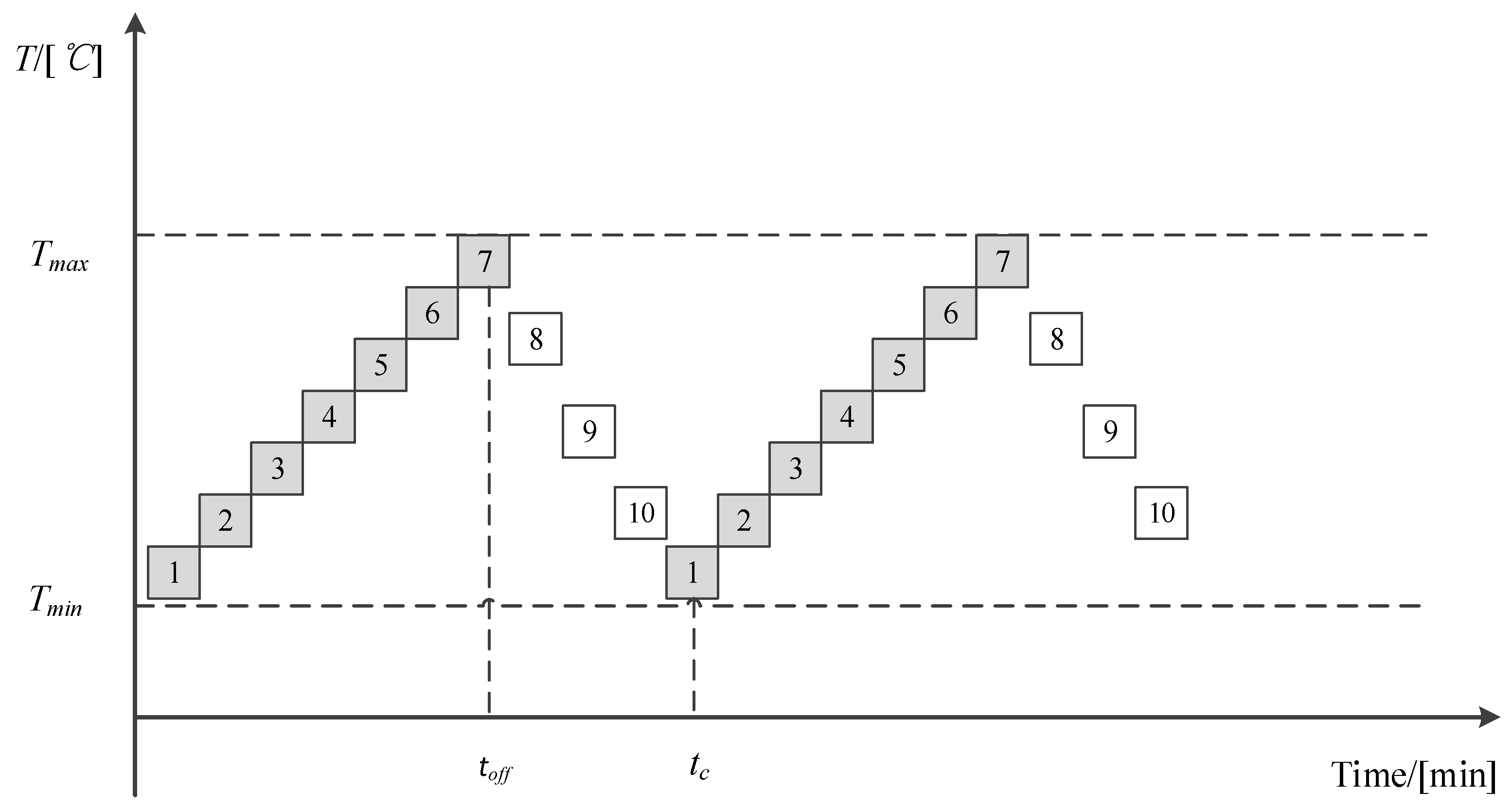
Figure 1 shows the states of a single air-conditioning unit during two operational cycles. As shown in the figure, there are 10 states of equal duration in an operational cycle. Seven shaded boxes represent “off” states and three white boxes represent “on” states. If the ambient temperature and set point remain unchanged, then the state of air-conditioning unit will switch forward from state 1 to state 10 in a temperature range of [Tmin, Tmax].
Assuming that there are NAC air-conditioning units with similar thermal parameters and the same initial thermal states shown in Figure 1, they are uniformly divided into tc groups, and each group is controlled in turn (as shown in Figure 1). If the state time interval Δt is 1 min, then at each moment, there are ton groups of ACLs that are “on” states and toff groups of ACLs that are “off” states in the temperature interval [Tmin, Tmax]. The total number of controlled groups/states equals to the sum of ton and toff. Thus, the power of the aggregated ACLs PACsum can be calculated as follows:
2.3. Virtual Power Plant Model for ACL
With the adjustment of temperature setting of ACLs, the aggregated demands will vary accordingly. In order to preferably integrate ACLs into the real-time scheduling and operation, the concept of VPP is used to represent the aggregated air-conditioning resources.
A VPP is comparable to a conventional power plant with its own operating characteristics, such as scheduling characteristics of generation, generation limits, and operating costs. Assuming that the ACLs with uniform and similar parameters can be equivalent to a virtual power plant. All of the ACLs in scheduling plans are divided into Ng VPPs. Before operators make the scheduling decisions, aggregators need to offer the feasible power regulation schemes and the corresponding compensation costs to the grid company. Let Ns,n denote the set of feasible power regulation schemes for VPP n. The real power of VPP n at time t is as follows:
where Pa,n,s refers to the load shedding of VPP n as it carries out scheme s at time t. The value of Sn,s,t is 0 or 1. When Sn,s,t = 1, VPP n implements the regulation scheme s at time t. While Sn,s,t = 0, VPP n does not implement the regulation scheme s at time t. As an example, when the set point of VPP n is adjusted from Tset to Treset, load consumptions in Tset and Treset can be, respectively, calculated according to (5). Subsequently, load shedding of VPP n in the above scenario can be obtained as:
where Pa,n,reset,t refers to load shedding of VPP n at time t when set point changes from Tset to Treset, and PACsum,n,reset,t and PACsum,n,set,t represent load consumptions of VPP n at time t in set point Treset and set point Tset., respectively.
2.4. Cost Calculation for VPP
As the temperature set point increases, the comfort of customers weakens. Thus, customers may obtain more compensation to remedy the reduction of comfort.
The operating cost of VPP n is defined as,
where K is the cost coefficients and ΔTn,s represents the absolute value of the set point variation for VPP n as it carries out scheme s. For example, if the set point of VPP n is adjusted from Tset to Treset, ΔTn,s is equal to |Treset − Tset|.
3. Load Equilibrium Entropy
The increasing peak-valley gap has brought enormous challenges to the reliable operations of the power systems. Many methods have been used to reduce the peak-valley gap, such as DR resources and ESSs. Although the peak-valley gap shrinks much after implementing load curtailment measures, the optimized load curve always appears to be multi-peak or concave-convex. How to make load evenly distributed during dispatch period through optimization measures is the goal of this paper in order to achieve optimal allocation of electric energy and improve the efficiency of electrical consumption. For this purpose, a new index is needed to evaluate the load equilibrium. In this paper, we propose a concept of load equilibrium entropy to quantify the overall equilibrium of the load curve.
As a widely-used concept in information theory, entropy can be adopted to measure heterogeneity [30]. For example, Bao et al. [31] evaluated the heterogeneity of power flow distribution over lines with entropy. In a similar way in this paper, we utilize entropy to assess load equilibrium during dispatch period.
The load curve follows continuous distribution patterns. For ease of calculation, we discretize the load curve. According to the definition of discrete information entropy, the discrete information source X can be calculated as follows:
where pi is the probability of occurrence of the i-th possible value of the source symbol. H uses a logarithm of base 2 and its unit is bit. In addition, .
There are two types of discrete information entropy: entropy of real numbers and interval entropy [32].
In this paper, we attempt to optimize the load curve. It is impossible to divide a variational curve into intervals. Hence, we adopted the entropy of real numbers. pi refers to the percentage of the i-th information value in all the information value:
To calculate load equilibrium entropy, we need to calculate the load utilization rate first.
where PL,t is the load at time t after implementing demand response measures and storage energy devices. pL,t is load utilization rate at time t and refers to the electricity consumption situation for customer at time t.
Load equilibrium entropy can be calculated as follows:
From Formula (10), we can see that the load equilibrium entropy provides an average measure of load curve equilibrium. As load at every time is more close to each other, the value of load equilibrium entropy H is bigger. When the load curve is flat in some special situation, H gets maximum value. Obviously, this is an extreme case.
4. Optimal Dispatching Model
In this section, the intraday dispatching model of ADN is built to optimize the outputs of the wind farm and the PV power station, electrical energy purchased from the grid, as well as charge/discharge power of the ESS and the outputs of the VPPs. In previous researches that aim at peak load reduction, the general objective of dispatching model is to minimize the total operation cost or to minimize the difference between peak load and valley load. Nevertheless, these studies did not take a measure about improving the load profile. In order to reduce peak load, achieve even distribution of loads, and optimally allocate electric energy, a multi-objective optimal dispatch model is presented based on load equilibrium entropy. The objective function of the proposed model contains the minimization of the operation costs and the maximization of load equilibrium entropy. We also simulate and compare the proposed model with other two models whose optimal objectives, respectively, are to minimize the scheduling cost of distribution system and maximize load equilibrium entropy.
4.1. Objective Functions and constraints
4.1.1. Model 1
The objective function of Model 1 is to maximize load equilibrium entropy:
Constraints include:
- (1)
- Power Balancewhere PW,t and PPV,t refer to the real power of the wind farm and the PV power station at time t; PTR,t is electrical energy purchased from the grid; Pload,t is the original system load at time t; PTOU,t represents load variation on account of TOU tariff; PE,t refers to the charge/discharge power of the storage battery at time t; PVPP,n,t is the real power of VPP n at time t.
- (2)
- The Upper and Lower Limit Constraints of Wind Farm and PV Power Stationwhere PWmax,t and PPVmax,t refer to the largest predictive power output of wind farm and PV power station at time t.
- (3)
- Constraint of Electrical Energy Purchased from the Gridwhere PTRmax,t is the largest energy purchased from the upper grid company.
- (4)
- Constraints of ESSTake the storage battery for example. The battery balance for ESS can be formulated as:where Et and Et−1, respectively, are capacity of the storage battery at time t and time t − 1. PE,t−1 represents the charge/discharge power at time t − 1.The charge/discharge limit for the storage battery can be represented by:where PEmax refers to maximum limit of charge power of the storage battery.The storage battery capacity limit can be represented as:where Emax and Emin refer to maximum and minimum values of capacity of the storage battery.
- (5)
- Constraints of VPPsAccording to the Formulas (4) and (5), the real power of VPPs can be calculated. We assume that the temperature regulation schemes are given before dispatching, and that the temperature set point does not continuously change. The real power of VPPs can be seen as the discrete variable.
4.1.2. Model 2
The objective function of Model 2 is to minimize the total operational cost of the distribution system, which includes electricity expenses due to purchasing electricity from wind farm, PV power station and the upper grid company, maintenance cost of ESS, and the operating cost of VPPs.
where CW, CPV and CTR, respectively, refers to electricity price of wind farm, PV power station and transmission grid, and CE is the operating cost of ESS.
4.1.3. Model 3
The dispatch problem of Model 3 is a multi-objective optimization, in which the operation cost is minimized and load equilibrium entropy is maximized. The objective functions can be formulated as follows:
4.2. Solution Method
We employ Particle Swarm Optimization algorithm to solve the three models because this algorithm can handle well the nonlinear mixed integer problem and has higher rate of convergence than other intelligent algorithms. Particle Swarm Optimization algorithm is also considered as one of the most promising method of optimizing problems with multiple objectives. The multi-objective optimization problems can be expressed as follows:
where x = [x1, x2, …, xn] refers to N-dimensional decision variable. Ωn is the feasible solution space of decision variables. fm(x) is the m-th objective function. M refers to the number of objective functions.
In the multi-objective optimization problems, the goals of each objective might be conflicting. It is hard to make all of the objectives simultaneously optimal. Therefore, we may get a set of optimal solutions for solving multi objective problems.
Assume that x1 and x2 are two feasible solution of multi objective optimization. Then, x1 dominates x2, when and only when the following two formulas are satisfied:
In this paper, according to Pareto dominance relations, we use Particle Swarm Optimization algorithm to obtain the Pareto optimal solutions [33,34]. Then, we choose the optimal compromise solution from a set of Pareto optimal solutions. In order to achieve such a compromise solution, a fuzzy decision making function with a membership function is adopted to represent the optimality of each objective function among every Pareto solution. The membership function for the j-th objective function among the i-th Pareto solution can be formulated as follows:
where fij refers to the i-th Pareto solution of the j-th objective function, fjmin and fjmax, respectively, are minimum and maximum values of the j-th objective function among all od the Pareto solutions, uij ranges from 0 to 1, where uij = 0 indicates that the decision maker is completely dissatisfied, while uij = 1 means that the decision maker is fully satisfied. For the i-th Pareto solution, the normalized membership function can be calculated as follows:
where I is the number of Pareto solutions. The maximum value of the membership function ui is the best compromise solution.
5. Case Study and Simulation Results
In this section, the simulation case is an active distribution system characterized by the inclusion of the wind farm, the PV power station, the storage unit and a significant number of TCLs. In the calculation, the time-steps are set as 15 min.
5.1. Basic Data
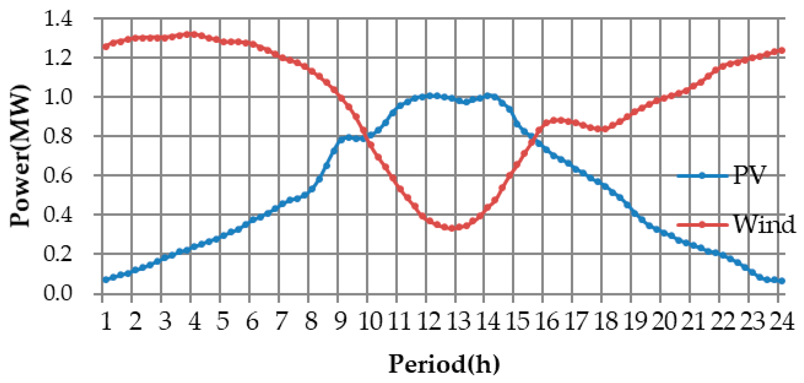
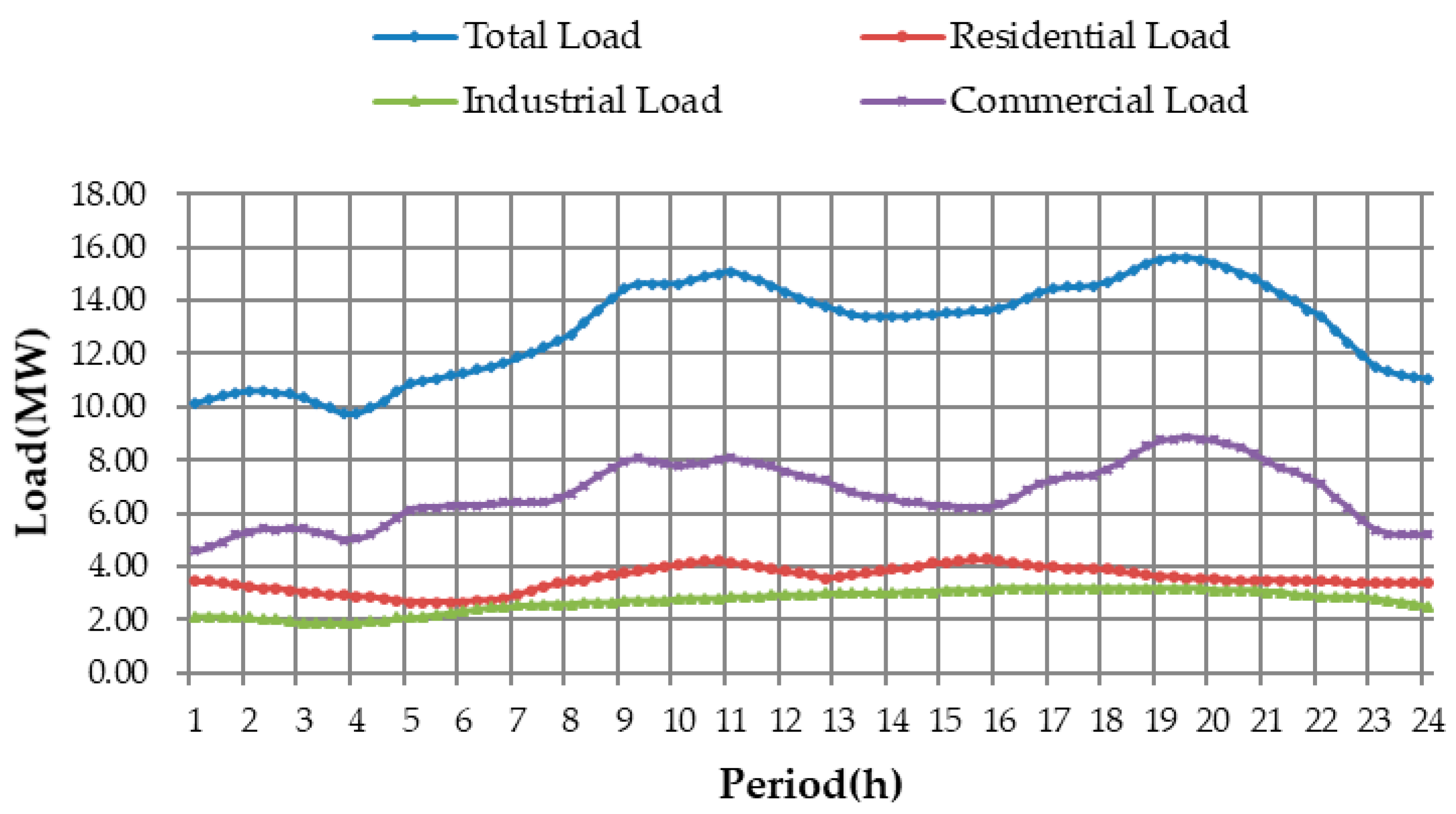
Figure 2 shows the power prediction curves of wind farm and PV power station. The max installed capacities of wind farm and PV power station are 1.5 MW and 1.2 MW, respectively. Based on their max installed capacities, we obtain prediction powers of wind and PV by transforming the data from [35]. Figure 3 illustrates four load curves, which, respectively, express initial system total load, residential load, commercial load, and industrial load of a typical day in the summer. According to the distributed generation pricing policy issued by National development and reform commission of China in 2011, it is assumed that the electricity prices of wind farm and PV power station are 510 RMB yuan/MWh and 1100 RMB yuan/MWh, respectively. The electricity price of power transmission network is 350 RMB yuan/MWh [36]. In our simulation study, we adopt the TOU pricing from [37]. TOU prices are composed of three price levels in one day, 150 RMB yuan/MWh during valley periods, 400 RMB yuan/MWh during plan periods, and 500 RMB yuan/MWh during peak periods. The division of the three periods is shown in Table 1. As can be seen in Figure 3, the system contains three types of costumers: residential costumer, industrial costumer, and commercial costumer. On account of the research on different load response of residential, industrial, and commercial costumer to TOU pricing [38], it can be seen that, in order to decrease their electricity costs, residential users tend to utilize more electricity in off-peak periods and less electricity in peak periods. By contrast, industrial users use much more electricity in off-peak periods, while their electricity consumption during peak hours is significantly decreased. For business users, they do not adjust their electricity consumption patterns much during office hours. Hence, we assume that the demand of commercial costumer is inelastic. We set the parameter value of residential demand elasticity and industrial demand elasticity as −0.36 and −0.48. Table 2 shows the parameters of ESS, which includes the maximum value of charge power, the initial capacity, and the total capacity of ESS.
We consider that load aggregators (LAs) [39,40,41] operate in our research district. LA provides a significant load reduction capacity to power network, according to dispatching commands by implementing the corresponding control measures to electricity consumers with thermostatically controllable devices. The aim of this case study is to realize participation of TCLs in the intraday dispatch through the VPP. Here, our paper does not focus on the research of the optimal control schedules, and we assume that ACLs can immediately carry out the dispatching command without response delay time. Assuming that there are six VPPs, controllable devices belonging to the same VPP have the same load parameters. Load reduction is required in two periods: 9:00–11:00 and 19:00–20:00. In summer, outdoor temperature may have small changes during high temperature periods. Therefore, we assume that outdoor temperature remains the same from 9:00 to 11:00 and from 19:00 to 20:00. Outdoor temperature Tout is set at 36 °C. Table 3 presents the parameters of six VPPs. Based on content in Section 2, we can calculate the outputs of every VPP. We propose three temperature regulation schemes: (1) rising the temperature set point by 2 °C for a maximum of 90 min; (2) rising the temperature set point by 3 °C for a maximum of 60 min; and, (3) rising the temperature set point by 4 °C for a maximum of 30 min. Table 4 shows the outputs of every VPP under different temperature regulation.
5.2. Analysis of Results
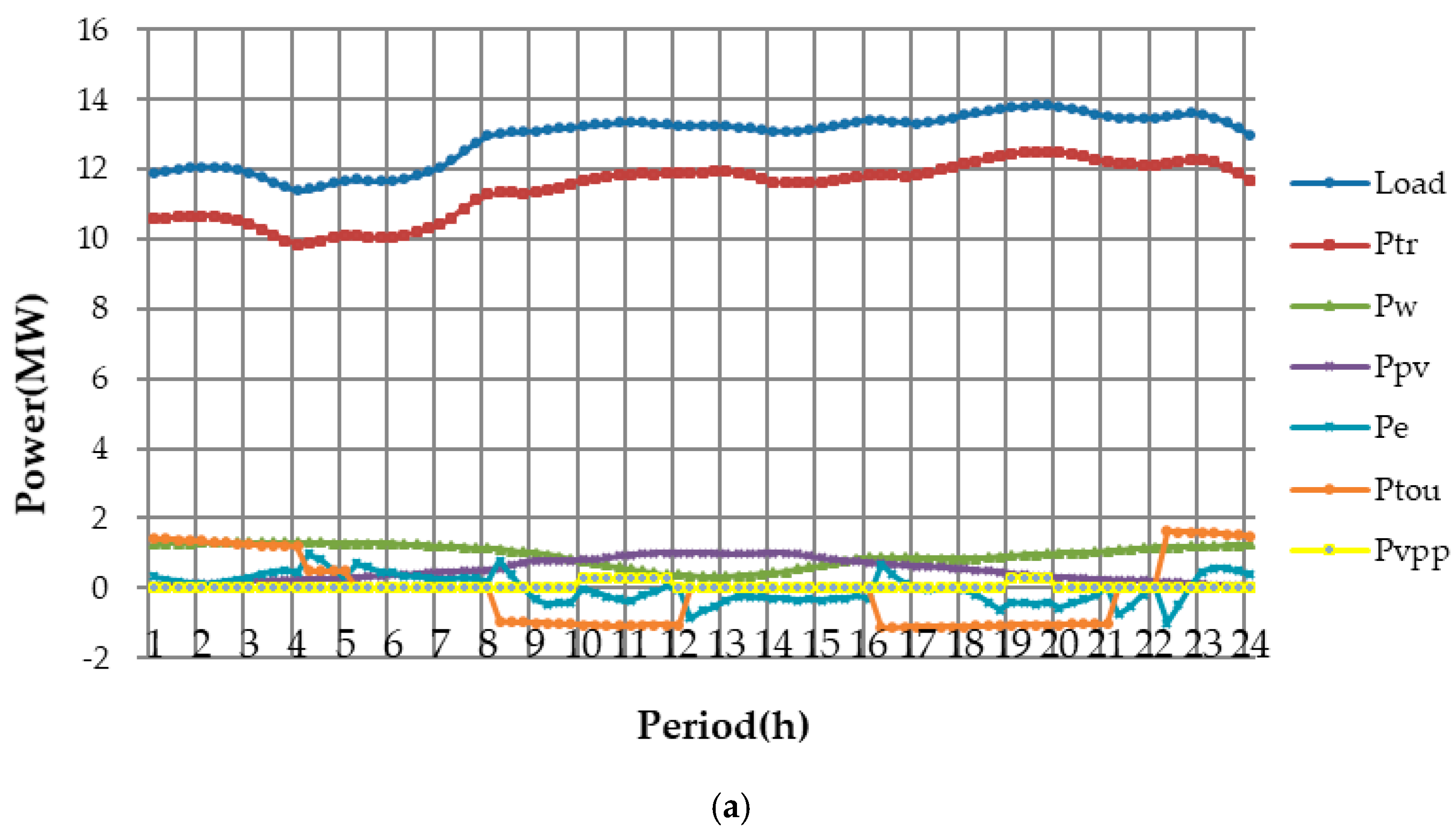
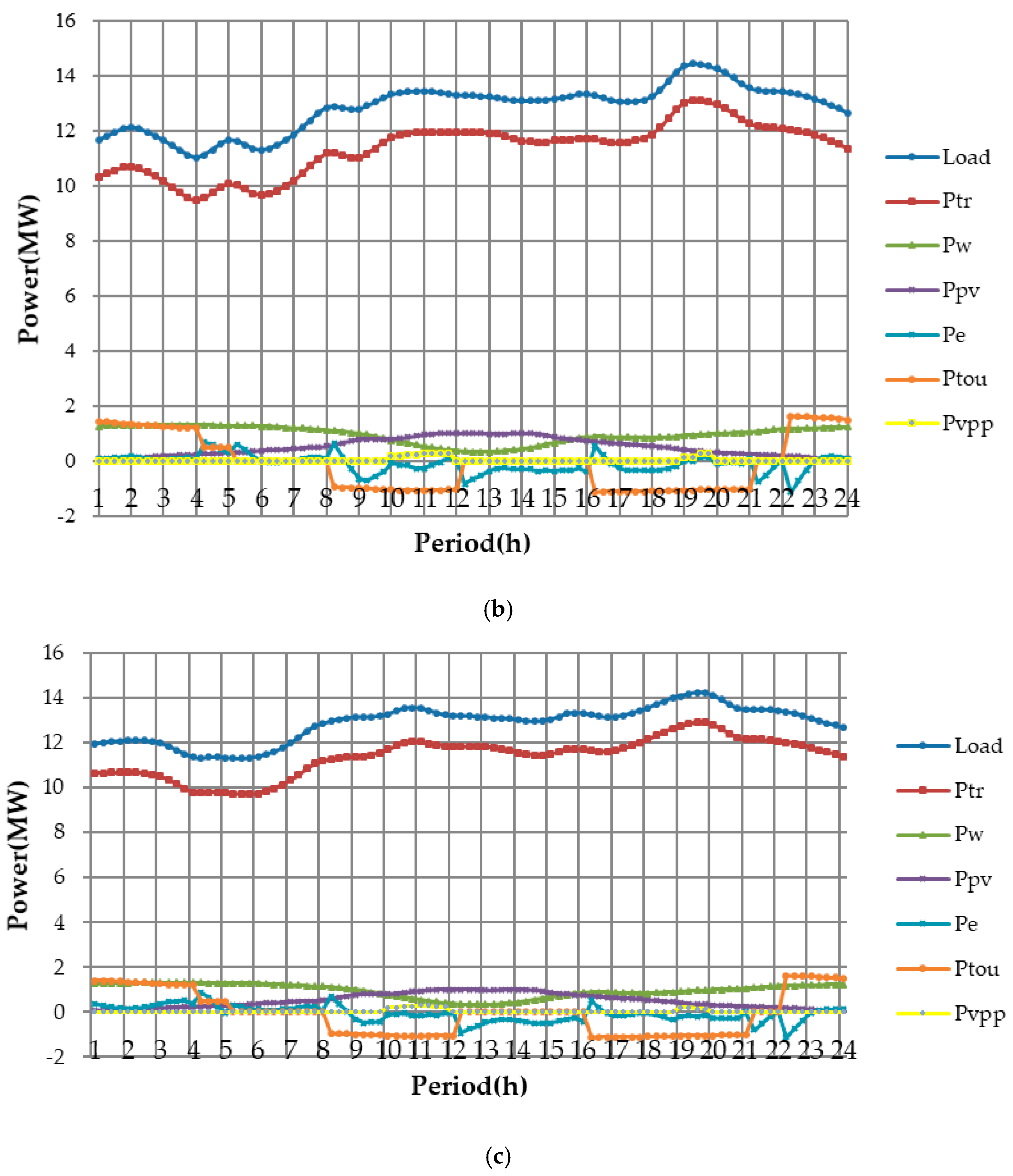
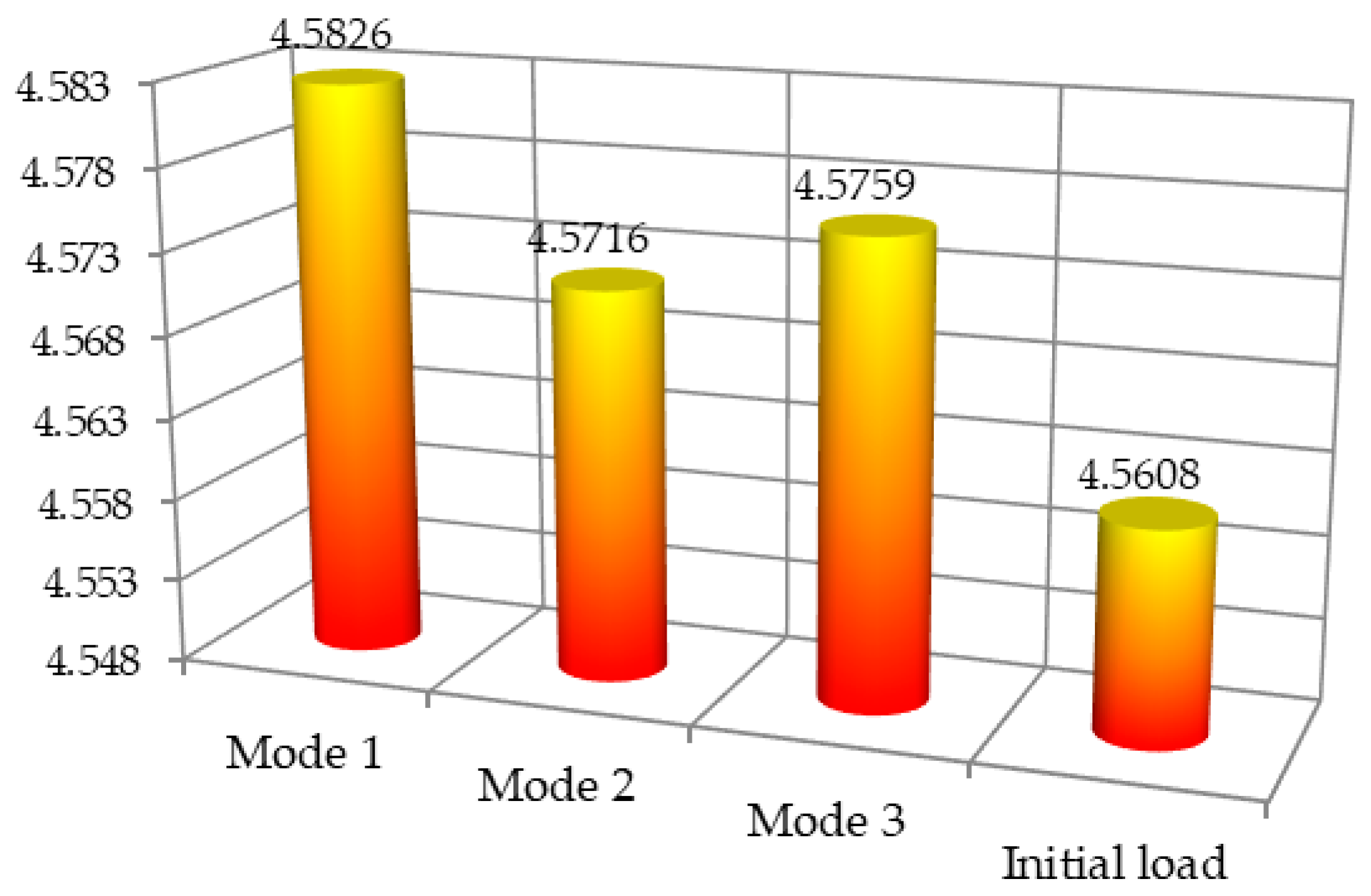
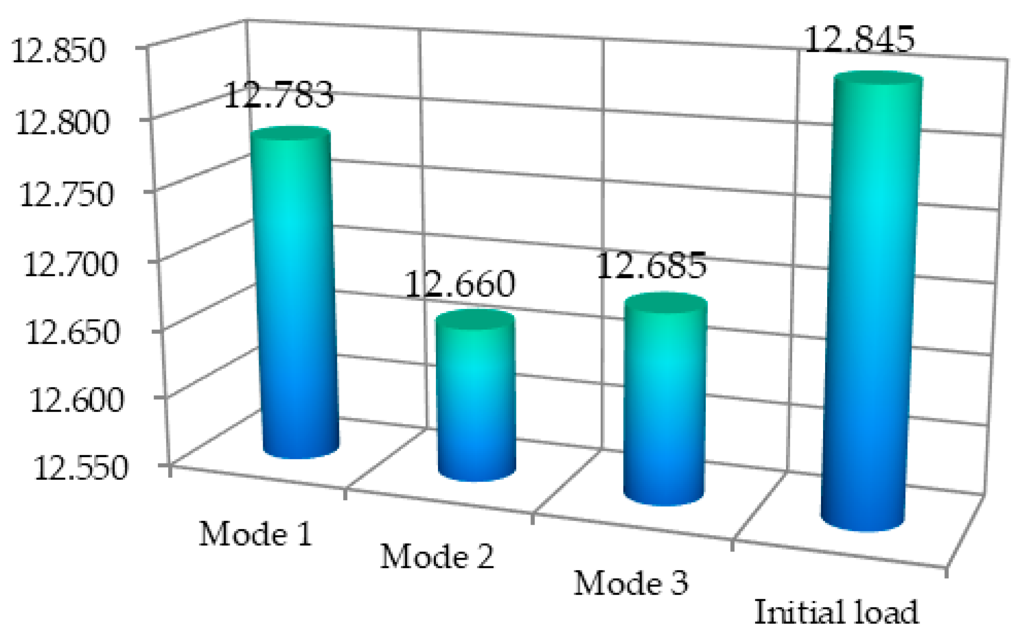
In this study, we simulate by using particle swarm optimization algorithm. We set that population size is 100 and the number of iteration is 300. The simulation is programmed in the MATLAB environment. Aiming at verifying the performance of the proposed load equilibrium entropy, we compare the proposed Model 3 with other two models. Figure 4 illustrates the optimized load curve, the output power of the wind farm and the PV power station, the power purchased from the grid, load variation due to TOU tariff, the charge/discharge power of the storage battery, and the output of VPPs under three models. When compared to the original scenario (Figure 3), when considering the energy storage and implementation of DR, the simulation results of load curves confirm that three models all accomplish the objective of decreasing the difference between peak and valley demand. Whereas, the distribution of load during whole dispatch period in mode 1 are more balanced than other two modes. In addition, Figure 5 also verifies this conclusion. Figure 5 shows the values of load equilibrium entropy of three optimized load curves and initial load equilibrium entropy. According to the presented definition of the load equilibrium entropy in Section 3, as the value of load equilibrium entropy increases, load at every time is close to equal. In Figure 5, the value of load equilibrium entropy of model 1 is at its maximum value, so the distribution of load is most equilibrium as compared to other models. The originally operation cost is 12.85 ten thousand RMB, when the system has not employed DR resources and storage energy devices. The total operation costs of three modes all decrease when compared to the original scenario, as shown in Figure 6. Because the objective of model 2 is to minimize the dispatch cost, the optimization scheme of model 2 is the most economical. Nevertheless, it can be observed that the load curve of mode 2 is the most fluctuant. By contract, the distribution of the improved load under model 1 is most balanced, but its operation cost is the maximum when compared with other two modes. To sum up, the best optimization scheme is model 3, which can balance the demands between economy and load equilibrium.
In order to compare the optimized index of load equilibrium with the conventional indices of load characteristics (peak load, valley load, the difference between peak and valley load, and load rate), we provide the values of characteristic indices and load equilibrium entropy of three optimized loads and initial load, as shown in Table 5. According to the previous simulation analysis based on Figure 4, the distribution of load under model 1 is most equilibrium among all of the models in the simulation. In addition, Table 5 shows that the other indices of load characteristics (peak load, valley load, the difference between peak and valley load, and load rate) of model 1 are also better than the other models. In addition, the conventional indices of load characteristics and the load equilibrium entropy of three optimized load results are better than that of the initial load, which is caused by the application of ESS and DR. Consequently, it is verified that DR resources and ESS technologies can play an important role in reducing peak demand, increasing the equilibrium level of load distribution and optimizing allocation of resources.
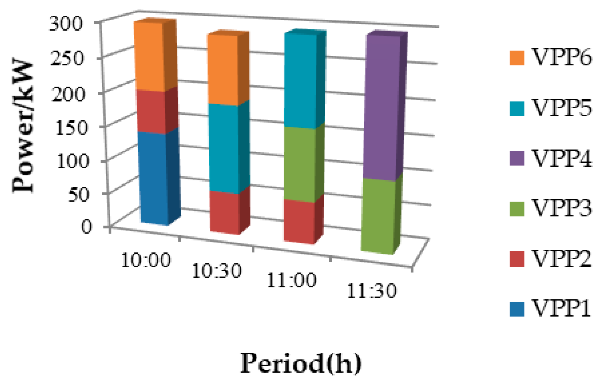
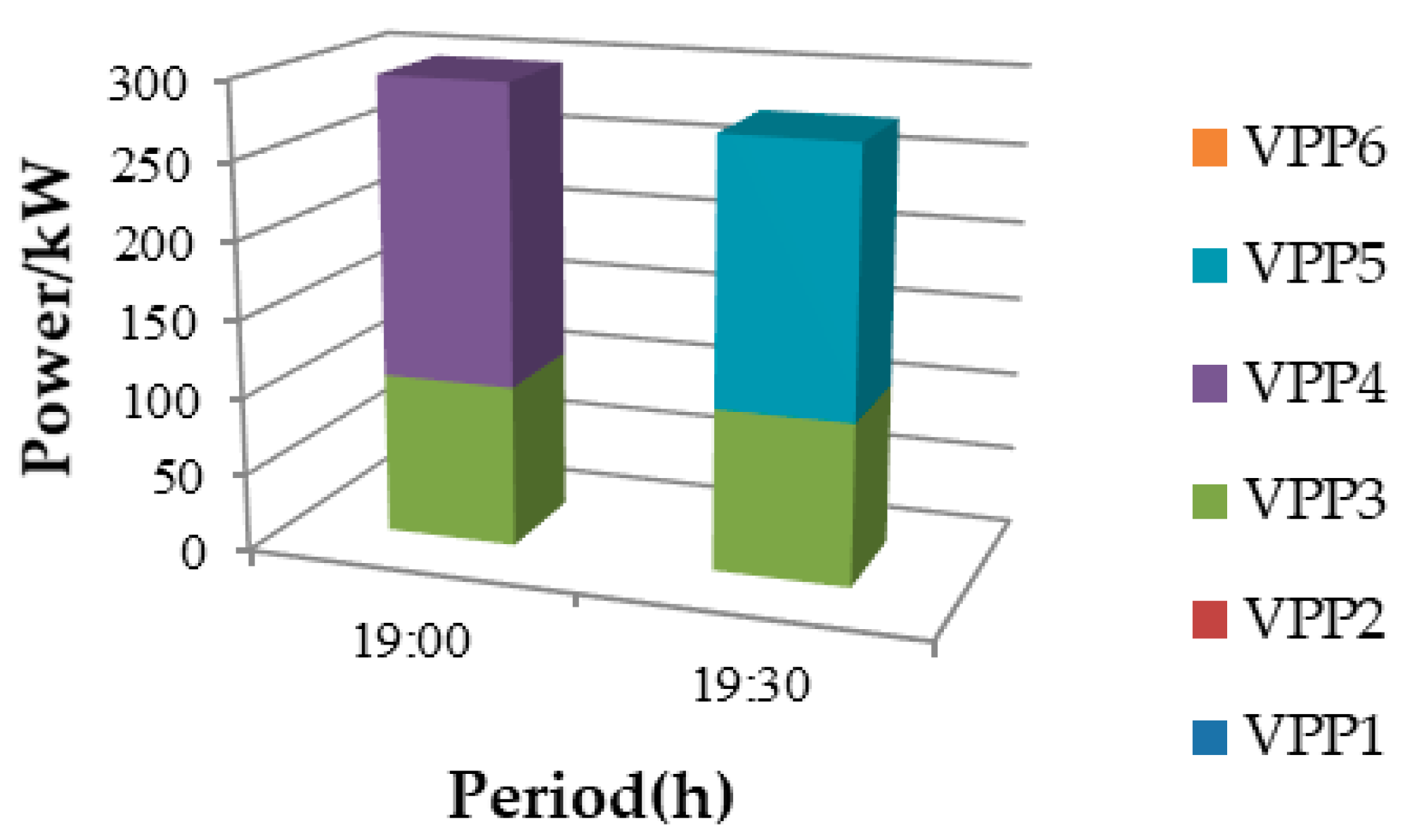
Taking Model 1 as an example, we analyze the optimization results of VPPs. Figure 7 shows the real power of 6 VPPs under Model 3 from 10:00 to 12:00. It includes the optimal load reductions and their durations. As can be seen, the six VPPs all output power during this period. Table 6 displays the output of six VPPs and the total load reduction at every time during this period. Form Table 6, we can tell that the average load reduction is 292.3 kW, which represents a drop of approximately 1.88% of peak load (15.6 MW). Meanwhile, Figure 8 presents the output power of six VPPs from 19:00 to 20:00. VPP3, VPP4 and VPP5 offer power delivery. Table 7 shows the output of the three VPPs and the total load reduction at every time during this period. In this period, there is an average load reduction of 285.2 kW, which accounts for approximately 1.83% of peak load. It is confirmed that VPP of ACLs can supply a potential electric energy reduction of approximately 0.8698 MWh for the whole control period. This reduction occupies about 1.92 % of total electric energy from 10:00 to 12:00 and from 19:00 to 20:00.
6. Conclusions
The integration of intermittent renewable energy advances the development of ADNs. Operation optimization, the core of ADNs’ active power management, makes ADNs different from the traditional distribution network. In this paper, a multi-objective optimization model for ADNs intraday dispatching is developed.
- The main contributions of this study are highlighted as follows:
- (1)
- It proposes a concept of load equilibrium entropy to quantify the overall equilibrium of a load curve.
- (2)
- It presents a VPP model of TCLs and the calculation method of VPP generation limits and operating costs. This model and method make it possible to integrate the VPP model into an optimization objective and constraints.
- (3)
- Based on the proposed load equilibrium entropy and the VPP model of TCLs, it builds a novel multi-objective optimal dispatching model of ADNs to implement the coordinated optimization of DERs, DR resources, and the energy storage systems.
- In addition, certain implications can be drawn from the simulation results:
- (1)
- The proposed dispatching model is effective in cost reduction of system operations, peak load curtailment, and efficiency improvement.
- (2)
- The results also confirm that the load equilibrium entropy index is viable to represent the equilibrium characteristic of load.
- (3)
- The simulate results illustrate that TCLs provide a reduction of approximately 1.92 % of total electric energy for the whole control period. This indicates that TCLs have a good potential in efficiency improvement and peak load curtailment.
Acknowledgments
This work was supported by National Key Research and Development Program (2016YFB0901104) and National Natural Science Foundation of China (51577061).
Author Contributions
The paper was a collaborative effort between the authors. Xiao Han carried out the main research tasks and wrote the full manuscript. Ming Zhou provided the original idea. Gengyin Li proposed very helpful suggestions during the whole process. Kwang Y. Lee helped to largely improve the whole manuscript.
Conflicts of Interest
The authors declare no conflict of interest.
Nomenclature
| RE | Renewable Energy |
| ESS | Energy Storage Systems |
| TCL | Thermostatically Controlled Load |
| VPP | Virtual Power Plant |
| PV | Photovoltaic |
| ADN | Active Distribution Network |
| DER | Distributed Energy Resource |
| TOU | Time-of-Use |
| ACL | Air Conditioning Load |
| SQ | State Queueing |
| LA | Load Aggregator |
References
- Sun, X.; Zhang, B.; Tang, X.; Mclellan, B.; Höök, M. Sustainable energy transitions in china: Renewable options and impacts on the electricity system. Energies 2016, 9, 980. [Google Scholar] [CrossRef]
- Warner, K.; Jones, G. The climate-independent need for renewable energy in the 21st century. Energies 2017, 10, 1197. [Google Scholar] [CrossRef]
- National Bureau of Statistics of China. China Statistical Yearbook 2016. 2016. Available online: http://www.stats.gov.cn/tjsj/ndsj/2016-/indexch.htm (accessed on 12 October 2016).
- NDRC Energy Research Institute. China 2050 High Renewable Energy Penetration Scenario and Roadmap Study; NDRC: Beijing, China, 2015. (In Chinese)
- Sun, B.; Yu, Y.; Qin, C. Should china focus on the distributed development of wind and solar photovoltaic power generation? A comparative study. Appl. Energy 2017, 185, 421–439. [Google Scholar] [CrossRef]
- Chen, F.; Liu, D.; Xiong, X. Research on Stochastic optimal operation strategy of active distribution network considering intermittent energy. Energies 2017, 10, 522. [Google Scholar] [CrossRef]
- Cong, P.; Tang, W.; Zhang, L.; Zhang, B.; Cai, Y. Day-ahead active power scheduling in active distribution network considering renewable energy generation forecast errors. Energies 2017, 10, 1291. [Google Scholar] [CrossRef]
- Gill, S.; Kockar, I.; Ault, G.W. Dynamic optimal power flow for active distribution networks. IEEE Trans. Power Syst. 2014, 29, 121–131. [Google Scholar] [CrossRef] [Green Version]
- Li, G.; Bie, Z.; Xie, H.; Lin, Y. Customer satisfaction based reliability evaluation of active distribution networks. Appl. Energy 2016, 162, 1571–1578. [Google Scholar] [CrossRef]
- Nick, M.; Cherkaoui, R.; Paolone, M. Optimal allocation of dispersed energy storage systems in active distribution networks for energy balance and grid support. IEEE Trans. Power Syst. 2014, 29, 2300–2310. [Google Scholar] [CrossRef]
- Valverde, G.; Cutsem, T.V. Model predictive control of voltages in active distribution networks. IEEE Trans. Smart Grid 2013, 4, 2152–2161. [Google Scholar] [CrossRef]
- Christakou, K.; Tomozei, D.C.; Boudec, J.Y.L.; Paolone, M. GECN: Primary voltage control for active distribution networks via real-time demand-response. IEEE Trans. Smart Grid 2014, 5, 622–631. [Google Scholar] [CrossRef]
- Chowdhury, S.P.; Chowdhury, S.; Crossley, P.A. Islanding protection of active distribution networks with renewable distributed generators: A comprehensive survey. Electr. Power Syst. Res. 2009, 79, 984–992. [Google Scholar] [CrossRef]
- Huang, W.; Tai, N.; Zheng, X.; Fan, C.; Yang, X.; Kirby, B.J. An impedance protection scheme for feeders of active distribution networks. IEEE Trans. Power Deliv. 2014, 29, 1591–1602. [Google Scholar] [CrossRef]
- Golshannavaz, S.; Afsharnia, S.; Aminifar, F. Smart distribution grid: Optimal day-ahead scheduling with reconfigurable topology. IEEE Trans. Smart Grid 2014, 5, 2402–2411. [Google Scholar] [CrossRef]
- Siano, P.; Sarno, D. Assessing the benefits of residential demand response in a real time distribution energy market. Appl. Energy 2016, 161, 533–551. [Google Scholar] [CrossRef]
- Safdarian, A.; Fotuhi-Firuzabad, M.; Lehtonen, M. A stochastic framework for short-term operation of a distribution company. IEEE Trans. Power Syst. 2013, 28, 4712–4721. [Google Scholar] [CrossRef]
- Bahramara, S.; Moghaddam, M.P.; Haghifam, M.R. A bi-level optimization model for operation of distribution networks with micro-grids. Int. J. Electr. Power Energy Syst. 2016, 82, 169–178. [Google Scholar] [CrossRef]
- Gabash, A.; Li, P. Active-reactive optimal power flow in distribution networks with embedded generation and battery storage. IEEE Trans. Power Syst. 2012, 27, 2026–2035. [Google Scholar] [CrossRef]
- Liu, J.; Zhang, L. Strategy design of hybrid energy storage system for smoothing wind power fluctuations. Energies 2016, 9, 991. [Google Scholar] [CrossRef]
- Torriti, J. Price-based demand side management: Assessing the impacts of time-of-use tariffs on residential electricity demand and peak shifting in Northern Italy. Energy 2012, 44, 576–583. [Google Scholar] [CrossRef]
- Lu, N.; Zhang, Y. Design considerations of a centralized load controller using thermostatically controlled appliances for continuous regulation reserves. IEEE Trans. Smart Grid 2013, 4, 914–921. [Google Scholar] [CrossRef]
- He, H.; Sanandaji, B.M.; Poolla, K.; Vincent, T.L. Aggregate flexibility of thermostatically controlled loads. IEEE Trans. Power Syst. 2015, 30, 189–198. [Google Scholar]
- Zhang, Q. The Successful Implementation of Household Air Conditioning Load Characteristic Test in Shanghai Grid. Available online: http://www.sh.sgcc.com.cn/load.LoadPage.d?siteCode=sdsd&newsid=1646947&page=detail_zxzx.xml (accessed on 18 March 2013).
- Ruiz, N.; Cobelo, I.; Oyarzabal, J. A direct load control model for virtual power plant management. IEEE Trans. Power Syst. 2009, 24, 959–966. [Google Scholar] [CrossRef]
- Pandžić, H.; Morales, J.M.; Conejo, A.J.; Kuzle, I. Offering model for a virtual power plant based on stochastic programming. Appl. Energy 2013, 105, 282–292. [Google Scholar] [CrossRef]
- Katipamula, S.; Lu, N. Evaluation of residential HVAC control strategies for demand response programs. ASHRAE Trans. 2006, 112, 535–546. [Google Scholar]
- Lu, N. An evaluation of the HVAC load potential for providing load balancing service. IEEE Trans. Smart Grid 2012, 3, 1263–1270. [Google Scholar] [CrossRef]
- Lu, N.; Chassin, D.P. A state-queueing model of thermostatically controlled appliances. IEEE Trans. Power Syst. 2004, 19, 1666–1673. [Google Scholar] [CrossRef]
- Cancho, R.F.I.; Solé, R.V. Optimization in Complex Networks. Lect. Notes Phys. 2003, 25, 114–125. [Google Scholar]
- Bao, Z.J.; Cao, Y.J.; Wang, G.Z.; Ding, L.J. Analysis of cascading failure in electric grid based on power flow entropy. Phys. Lett. A 2009, 373, 3032–3040. [Google Scholar] [CrossRef]
- Jin, B.; Zhang, B.; Wang, K. Entropy theory based optimal power flow balancing analysis in power system. Autom. Electr. Power Syst. 2016, 40, 80–86. [Google Scholar]
- Aghajani, G.R.; Shayanfar, H.A.; Shayeghi, H. Presenting a multi-objective generation scheduling model for pricing demand response rate in micro-grid energy management. Energy Convers. Manag. 2015, 106, 308–321. [Google Scholar] [CrossRef]
- Yang, J.; Zhou, J.; Liu, L.; Li, Y. A novel strategy of pareto-optimal solution searching in multi-objective particle swarm optimization (MOPSO). Comput. Math. Appl. 2009, 57, 1995–2000. [Google Scholar] [CrossRef]
- Gao, Y.; Li, R.; Liang, H.; Zhang, J.; Ran, J.; Zhang, F. Two step optimal dispatch based on multiple scenarios technique considering uncertainties of intermittent distributed generations and loads in the active distribution system. Proc. CSEE 2015, 35, 1657–1665. [Google Scholar]
- Gao, Y. Research on Intentional Islanding and Day ahead Schedule Optimal Dispatch of Active Distribution Network. Ph.D. Thesis, China Agricultural University, Beijing, China, 2013. [Google Scholar]
- Ai, X.; Zhou, S.; Zhao, Y. Study on time of use pricing of user side considering wind power uncertainty. Power Syst. Technol. 2016, 40, 1529–1535. [Google Scholar]
- Yang, P.; Tang, G.; Nehorai, A. A game-theoretic approach for optimal time-of-use electricity pricing. IEEE Trans. Power Syst. 2013, 28, 884–892. [Google Scholar] [CrossRef]
- Chae, J.; Joo, S.K. Demand response resource allocation method using mean-variance portfolio theory for load aggregators in the korean demand response market. Energies 2017, 10, 879. [Google Scholar] [CrossRef]
- Gkatzikis, L.; Koutsopoulos, I.; Salonidis, T. The role of aggregators in smart grid demand response markets. IEEE J. Sel. Area Commun. 2013, 31, 1247–1257. [Google Scholar] [CrossRef]
- Wu, D.; Aliprantis, D.C.; Ying, L. Load scheduling and dispatch for aggregators of plug-in electric vehicles. IEEE Trans. Smart Grid 2012, 3, 368–376. [Google Scholar] [CrossRef]
Figure 1.
State-queueing model of air conditioning load (ACL).

Figure 2.
Power prediction curves of wind farm and photovoltaic (PV) power station.

Figure 3.
Initial system load curves.

Figure 4.
The optimized system load curve, the output power of the wind farm and the PV power station, the power purchased from the grid load variation on account of TOU tariff, the charge/discharge power of the storage battery and the output of VPPs under three models. (a) Model 1; (b) Model 2; (c) Model 3.


Figure 5.
The values of load equilibrium entropy under three models and initial load.

Figure 6.
The total operation costs of three models and the original operation cost (unit: ten thousand RMB).
Figure 6.
The total operation costs of three models and the original operation cost (unit: ten thousand RMB).

Figure 7.
The output of six VPPs under Model 1 from 10:00 to 12:00.

Figure 8.
The output of six VPPs under Model 1 from 19:00 to 20:00.


Table 1.
Electricity prices of time-of-use (TOU) pricing.
| TOU Prices | Periods | Prices (RMB/(MWh)) |
|---|---|---|
| Peak load | 9:00–12:00 and 17:00–22:00 | 500 |
| Plan load | 6:00–8:00 and 13:00–16:00 | 400 |
| Valley load | 1:00–5:00 and 23:00–24:00 | 150 |
Table 2.
Parameters of energy storage systems (ESS).
| Parameters | Values |
|---|---|
| Maximum charge power (MW) | 0.5 |
| Initial capacity (MWh) | 1.0 |
| Total capacity (MWh) | 5.5 |
Table 3.
Parameters of six virtual power plant (VPPs).
| Parameters | R (°C/kW) | C (kWh/°C) | PAC (kW) | η | NAC |
|---|---|---|---|---|---|
| VPP1 | 3.5 | 12.1 | 3.5 | 2.5 | 480 |
| VPP2 | 2.0 | 10.0 | 2.5 | 2.7 | 460 |
| VPP3 | 2.5 | 11.6 | 3.0 | 2.6 | 500 |
| VPP4 | 2.7 | 12.8 | 4.5 | 2.1 | 560 |
| VPP5 | 2.7 | 15.8 | 4.2 | 2.3 | 540 |
| VPP6 | 2.8 | 13.5 | 2.9 | 2.8 | 500 |
Table 4.
Output of VPP under different schemes.
| Schemes | +2 °C | +3 °C | +4 °C |
|---|---|---|---|
| Duration | 90 min | 60 min | 30 min |
| VPP1 | 69.3 kW | 102.9 kW | 138.6 kW |
| VPP2 | 61.5 kW | 92.2 kW | 123.0 kW |
| VPP3 | 69.4 kW | 104.1 kW | 138.8 kW |
| VPP4 | 96.2 kW | 144.4 kW | 192.6 kW |
| VPP5 | 84.7 kW | 127.1 kW | 169.5 kW |
| VPP6 | 64.5 kW | 96.7 kW | 129.0 kW |
Table 5.
Indices of load characteristics.
| Model | Peak Load (MW) | Valley Load (MW) | Peak-Valley Gap (MW) | Load Rate (%) | Load Equilibrium Entropy |
|---|---|---|---|---|---|
| Model 1 | 13.80 | 11.43 | 2.38 | 93.5 | 4.5826 |
| Model 2 | 14.37 | 11.03 | 3.34 | 89.2 | 4.5716 |
| Model 3 | 14.23 | 11.33 | 2.91 | 90.1 | 4.5759 |
| Initial load | 15.56 | 9.81 | 5.75 | 83.5 | 4.5608 |
Table 6.
The output of VPPs from 10:00 to 12:00.
| Period | Output of VPP1 (kW) | Output of VPP2 (kW) | Output of VPP3 (kW) | Output of VPP4 (kW) | Output of VPP5 (kW) | Output of VPP6 (kW) | Total Power (kW) |
|---|---|---|---|---|---|---|---|
| 10:00 | 138.6 | 61.5 | 0 | 192.6 | 0 | 96.7 | 296.8 |
| 10:30 | 0 | 61.5 | 0 | 0 | 127.1 | 96.7 | 285.3 |
| 11:00 | 0 | 61.5 | 104.1 | 0 | 127.1 | 0 | 292.7 |
| 11:30 | 0 | 0 | 104.1 | 0 | 0 | 0 | 296.7 |
Table 7.
The output of VPPs from 19:00 to 20:00.
| Period | Output of VPP3 (kW) | Output of VPP4 (kW) | Output of VPP5 (kW) | Total Power (kW) |
|---|---|---|---|---|
| 19:00 | 104.1 | 192.6 | 0 | 296.7 |
| 19:30 | 104.1 | 0 | 169.5 | 273.6 |
© 2017 by the authors. Licensee MDPI, Basel, Switzerland. This article is an open access article distributed under the terms and conditions of the Creative Commons Attribution (CC BY) license (http://creativecommons.org/licenses/by/4.0/).
Share and Cite
MDPI and ACS Style
Han, X.; Zhou, M.; Li, G.; Lee, K.Y. Optimal Dispatching of Active Distribution Networks Based on Load Equilibrium. Energies 2017, 10, 2003. https://doi.org/10.3390/en10122003
AMA Style
Han X, Zhou M, Li G, Lee KY. Optimal Dispatching of Active Distribution Networks Based on Load Equilibrium. Energies. 2017; 10(12):2003. https://doi.org/10.3390/en10122003
Chicago/Turabian StyleHan, Xiao, Ming Zhou, Gengyin Li, and Kwang Y. Lee. 2017. "Optimal Dispatching of Active Distribution Networks Based on Load Equilibrium" Energies 10, no. 12: 2003. https://doi.org/10.3390/en10122003
Note that from the first issue of 2016, this journal uses article numbers instead of page numbers. See further details here.