Investigation of Heat Pump Operation Strategies with Thermal Storage in Heating Conditions

Abstract

A heat pump with thermal storage system is a system that operates a heat pump during nighttime using inexpensive electricity; during this time, the generated thermal energy is stored in a thermal storage tank. The stored thermal energy is used by the heat pump during daytime. Based on a model of a dual latent thermal storage tank and a heat pump, this study conducts control simulations using both conventional and advanced methods for heating in a building. Conventional methods include the thermal storage priority method and the heat pump priority method, while advanced approaches include the region control method and the dynamic programming method. The heating load required for an office building is identified using TRNSYS (Transient system simulation), used for simulations of various control methods. The thermal storage priority method shows a low coefficient of performance (COP), while the heat pump priority method leads to high electricity costs due to the low use of thermal storage. In contrast, electricity costs are lower for the region control method, which operates using the optimal part load ratio of the heat pump, and for dynamic programming, which operates the system by following the minimum cost path. According to simulation results for the winter season, the electricity costs using the dynamic programming method are 17% and 9% lower than those of the heat pump priority and thermal storage priority methods, respectively. The region control method shows results similar to the dynamic programming method with respect to electricity costs. In conclusion, advanced control methods are proven to have advantages over conventional methods in terms of power consumption and electricity costs.

1. Introduction

Abnormal climatic conditions caused by global warming has increased the demand for cooling in summer and heating in winter; accordingly, electricity demand is continuously growing. Heating and cooling loads vary according to various factors, including solar radiation and outdoor temperatures, and reach maximum values at specific times, leading to peak electricity loads to meet heating and cooling demands [1,2]. Therefore, heating and cooling systems require efficient operation strategies to stabilize electricity demand and reduce the peak electricity usage [3].

A heat pump–thermal storage system is an effective technology for addressing the stabilization issue, as the system operates a heat pump during nighttime when the electricity demand is low [4]. It stores thermal energy for heating and cooling in the thermal storage tank and uses the stored energy during daytime when the higher loads occur. The type of thermal storage system depends on the operation modes and thermal storage materials. The operation modes are categorized into full thermal storage and partial thermal storage. In the former, all the heat required in daytime is stored at night, as opposed to about 40–50% in the latter. Thermal storage systems can be classified based on the thermal storage materials into water systems that store sensible heat of water, ice systems that freeze water and use its latent heat, and latent thermal storage systems that use the latent heat of other phase change materials (PCMs) [5,6]. Studies have been conducted on various types of thermal storage systems. Kim et al. [7] conducted performance experiments of a closed ice thermal storage system using screw capsules to calculate energy storage density and discharge efficiency. Yang et al. [8] studied storing and discharging characteristics of a dual thermal storage tank by applying low- and high-temperature PCMs, which are latent heat storage materials, to improve thermal storage density. Lee et al. [9] performed numerical analyses on discharging performance of a thermal storage tank with varying packing modules, examining the change in performance with different numbers of modules and different flow rates.

In heat pump systems with partial thermal storage, heating and cooling capacity of the thermal storage tank and heat pump should be controlled to respond to the varying heating and cooling loads [10]. Conventional control methods include the thermal storage priority method, where the heating and cooling loads below a specific level are first met by the thermal storage tank and the rest by the heat pump and the heat pump priority method, where the order of response is reversed so that the loads below a specific level are first met by the heat pump and the rest by the thermal storage tank. Efforts have been made to optimize the operational control of thermal storage systems using non-conventional methods [11]. Ahn et al. [12] analyzed the operational performance and costs of ice-on-coil thermal storage systems during the summer season, based on simulations, concluding that the chiller downstream method is more economical than other approaches. Spethmann et al. [13] made a comparative analysis of traditional control methods of ice thermal storage systems, suggesting that electricity pricing structure is the most influential factor in economic terms. Braun [14] examined two conventional control methods and optimal operational methods of ice thermal storage systems based on an electricity pricing scheme. Kintner-Meyer et al. [15] discussed design load and operational methods of the heat pump and thermal storage tank. Jung et al. [16] studied economical operational mechanism of ice thermal storage systems, considering cooling load variations, and suggested a control method combining the advantages of the thermal storage priority and chiller priority methods. Chen et al. [17], Chang et al. [18], Henze et al. [19], and Kirk et al. [20] established an operational strategy using dynamic programming, which minimizes cost functions and thus finds the optimized control path. In contrast, Lee et al. [21] showed that operating costs can be reduced by comparing the chiller priority method with the optimized control method, which minimizes costs using the dynamic programming method. As such, studies on optimizing thermal storage systems have focused on cooling systems using ice storage tanks, which are commonly used in practice, while that on heating systems using heat pumps has been insufficient.

More recently, heat pump-thermal storage heating systems have been considered as a solution to address electric load leveling issues stemming from heating and cooling peak demands, which occur both in winter and summer. Thermal storage tanks need to store thermal energy for cooling in summer, as opposed to thermal energy for heating in winter. Therefore, this study examines a system comprising a heat pump and a dual latent thermal storage. The dual latent thermal storage tank is equipped with cooling and heating PCMs having different phase change temperatures to be used for both cooling and heating operations.

This study focuses on the control method for the thermal storage tank and heat pump to optimize power consumption and electricity costs for heating, which have been explored relatively less than for cooling. A thermal performance model of the thermal storage tank is developed using the heat transfer model to reflect the characteristics of the PCMs for heating and cooling. The storage and discharge performance for heating is verified by comparing the modeled results with the experimental outcomes obtained from an actual thermal storage tank. The experiments of the heat pump performance are used to formulate a heat pump model, which can predict power consumption under different conditions in terms of water outlet temperature, outdoor temperature, and partial load operation. Using numerical models developed for the thermal storage tank and the heat pump, the power consumption and electricity costs of the heat pump during winter are analyzed and compared for different control methods, namely, conventional control methods, the region control method, and the dynamic programming method.

2. System Simulation Model

2.1. Target System

The heat pump-thermal storage system used in this study consisted of a heat pump and a thermal storage tank to meet the heating and cooling loads of a building, as described in Figure 1. As a result of previous studies, the heat pump was located downstream of the thermal storage tank to increase thermal energy utilization [22]. A bypass line was arranged in the thermal storage tank with an adjustable three-way valve. The circulation flow rate of the system was designed to be constant, but the changeable flow rate of water supplied to the tank allowed the system to control the heating capacity to accommodate the heating load of the building. PCM packs for heating and cooling were loaded inside the thermal storage tank.

The specifications and appearance of the cooling and heating PCM packs are presented in

Table 1. Specification of packed PCM (Phase change material).

Parameter	Specification
Type	Heating	Cooling
Thermal Conductivity of liquid (W/m·K)	0.167	0.136
Thermal Conductivity of solid (W/m·K)	0.346	0.307
Average phase change temperature (°C)	52	4
Heat of fusion (kJ/kg)	196.87	252.30
Specific heat of liquid (kJ/kg·K)	1.97	2.07
Specific heat of solid (kJ/kg·K)	2.30	2.32
Size (mm)	17.3 (W) × 250 (L) × 310 (H)
Pack weight (kg)	1

and Figure 2a. PCMs are organic n-tetradecane packed with polymer films in a rectangular shape. The cooling and heating PCMs have about 2 °C of transition temperature difference, however, constant phase temperatures are assumed as average temperatures of 4 °C and 52 °C for cooling and heating PCMs, respectively [23]. One pack weighs 1 kg, and measures 250 mm × 310 mm × 17.3 mm. As demonstrated in Figure 2b, The PCM packs are stacked to fill the interior of the thermal storage tank: six layers in height, eight layers in depth, and 28 layers in width. Thus, a total of 1344 packs of heating and cooling PCMs are used. As shown in Figure 2 and Figure 3, the packs are fixed vertically, preventing them from tilting and allowing efficient heat transfer during phase change [24]. Water flows inside pack spacing of 38.4 mm from top to bottom.

The thermal storage tank specifications, thermal storage conditions, and the amount of thermal energy stored for heating and cooling are summarized in

Table 2. Specification of thermal storage.

Parameter	Specification
Type	Heating	Cooling
Packed PCM (EA)	147	1197
Latent thermal storage energy (kJ)	28,940	302,000
Total thermal storage energy (kJ)	288,000	483,000
Operating temperature range (°C)	40–55	2–12
Size (mm)	1750 (W) × 2000 (L) × 2000 (H)
Volume (m3)	5.616

. The specifications were determined considering heating and cooling loads during winter and summer and thermal storage conditions. The total thermal energy storage for cooling is 483 MJ, which is calculated from the sensible heat capacity and latent heat capacity of the heating and cooling PCMs and the sensible heat capacity of water as Equations (1)–(4). The total thermal energy storage for heating is calculated as 288 MJ using the same equations. In the equations, $\Delta T_{st}$ means the maximum possible temperature difference of thermal storage by the operating temperature range as shown in Table 2. In this study, $\Delta T_{st}$ is 15 °C for heating. The design cooling load during summer is greater than the heating load during winter in Seoul; hence, the total thermal energy storage for cooling is greater than that for heating. The heat pump system in this study is partial thermal storage, where the heating capacity meets 40% of the average heating load for the day.

$$Q_{st}=Q_{w,sen}+Q_{p,sen}+Q_{p,lat}$$

(1)

$$Q_{w,sen}=M_w{C}_{p,w}\Delta T_{st}$$

(2)

$$Q_{p,sen}=M_{pc}{C}_{p,p}\Delta T_{st}+M_{ph}{C}_{p,p}\Delta T_{st}$$

(3)

$$Q_{p,lat}=h_{fg}{M}_{SPF}$$

(4)

Figure 3 indicates the control volume for the numerical analysis of thermal storage. The water supplied to the thermal storage tank was uniformly distributed along the interior of the tank from a diffuser located at the top, and discharged from the bottom. The numerical models of the thermal storage tank were categorized into the sensible heat transfer process of heating and cooling PCMs in their solid and liquid conditions or the latent heat transfer process at phase-change temperature.

Uniform properties at each control volume are assumed in the 1-D lumped heat transfer model. The conduction heat transfer in the height direction is not considered, and the outlet water conditions of each control volume becomes the inlet water conditions of the next control volume. As for the sensible heat transfer process of the PCMs, the heat transfer between the PCM packs and circulating water can be expressed by Equations (5) and (6). The water at each control volume is assumed to be fully mixed and outlet temperature is the same with bulk temperature of water as Equation (7). The governing equations are based on the energy balance between PCM packs and water as the temperature changes.

$${\rho }_p{V}_{p,cv}{C}_{p,p}\frac{d{T}_p}{dt}=U_s{\mathrm{A}}_p\left(T_w-T_p\right)$$

(5)

$${\rho }_w{V}_{w,cv}{C}_{p,w}\frac{d{T}_w}{dt}=U_s{\mathrm{A}}_p\left(T_p-T_w\right)+{\dot{m}}_w{C}_{p,w}\left(T_{in}-T_{out}\right)$$

(6)

$$T_{out}=T_w$$

(7)

$U_s$ indicates the sensible overall heat transfer coefficient between the PCM packs and circulating water, defined by the exterior convection heat transfer coefficient and internal conduction heat transfer coefficient of the PCM pack. The thickness of the packaging film is 0.1 mm and the conductive heat transfer resistance by packaging film comprises about 0.5% of the total heat transfer resistance, so conductive heat transfer resistance by the thin packaging film is neglected. In the sensible heat transfer process, the values presented in Table 1 were used as the PCM parameters depending on the type and phase of each material. Equations (8) and (9) describe the latent heat transfer process, while the governing equations are expressed using the energy balance equation reflecting the solid mass ratio, which changes during phase change, and the energy balance equation between the heating PCM packs and circulating water.

$${\mathrm{h}}_{fg}\frac{d{M}_{SPF}}{dt}=U_l{\mathrm{A}}_p\left(T_p-T_{out}\right)+{\dot{m}}_w{C}_{p,w}\left(T_{in}-T_{out}\right)$$

(8)

$${\rho }_w{V}_{w,cv}{C}_{p,w}\frac{d{T}_w}{dt}=U_l{\mathrm{A}}_p\left(T_p-T_{out}\right)+{\dot{m}}_w{C}_{p,w}\left(T_{in}-T_{out}\right)$$

(9)

$U_l$ refers to the overall heat transfer coefficient when the heating PCMs are within the latent heat transfer region, which reflects the exterior convection heat transfer coefficient and internal convection heat transfer coefficient inside the phase-changing PCM packs. The internal heat transfer coefficient when the phase is changing depends on the storage and discharge processes. The Reynolds number of circulating water between PCM packs is about 980 in this study. The exterior convection heat transfer coefficient between the PCM packs and circulating water is calculated using Equation (10), which is a heat transfer coefficient correlation for channel flow assuming laminar flow.

Equation (10) assumes that the six layers of PCM packs form a continuous long channel in the vertical direction, so it is assumed that boundary layer development is formed from the top. D and L represent the channel spacing between PCM packs (38.4 mm) and the length from top of PCM packs to the control volume, respectively.

$$Nu=\frac{h_{w}D}{k_w}=3.66+\frac{0.065\left(\frac{D}{L}\right)RePr}{1+0.04{[\left(\frac{D}{L}\right)RePr]}^{\frac{2}{3}}}$$

(10)

$$h_{SPF}=a_1+a_2\left(SPF\right)+a_3{\left(SPF\right)}^2+a_4{\left(SPF\right)}^3+a_5{\left(SPF\right)}^4$$

(11)

In the latent heat transfer process, the internal heat transfer coefficient is different for charging and discharging heat and depends on the solid packing factor (SPF) of the heating PCMs, as indicated in Equation (11) and

Table 3. Heat transfer coefficients of PCM at charging/discharging.

Coefficient	${\mathit{a}}_{\mathbf{1}}$	${\mathit{a}}_{\mathbf{2}}$	${\mathit{a}}_{\mathbf{3}}$	${\mathit{a}}_{\mathbf{4}}$	${\mathit{a}}_{\mathbf{5}}$
Charging	51	0.5	−154	235	−121
Discharging	5	141	−300	370	−143

. SPF is defined as the ratio of the mass of solid PCMs to the total PCM mass in the pack. When the PCMs in a pack are entirely fluid, SPF is equal to 0; when they are all solid, SPF is 1. This study utilizes the internal heat transfer coefficient model during the phase-change process, which was developed in a previous study [25].

A numerical analysis was performed with respect to the developed model of the thermal storage tank, using a MATLAB program [26]. A series of experiments were conducted on charge and discharge performance in a dual new latent heat storage tank with similar features to previous studies [27], and the outlet temperatures of the storage tank are shown in Figure 4. The experiments and simulations were performed for approximately 10 h. The operating conditions of the thermal storage tank are determined in accordance with midnight-electricity equipment technical specifications by Korea Electric Power Corporation (KEPCO) [5]. The initial interior temperature of the storage tank during the charge process was 40 °C, while the inlet water temperature was 55 °C. It was assumed that the charge process terminated when the outlet temperature of the storage tank reached 55 °C. Subsequently, the discharge process started with an inlet water temperature of 40 °C. When the outlet temperature of the storage tank reached 40 °C, the discharge process was completed. The forward difference method is used to simulate numerical models. Figure 5 shows the result of temperature estimation according to the time interval and the number of control volume in height at the moment of 5 h during charging process. The time interval is selected as 6 s and the thermal storage tank is divided into 60 control volumes in height [28]. Simulation models well predicted the outlet temperature of the thermal storage tank in the experiments, and the amount of heat charged and discharged coincided with that summarized in Table 2.

The heat pump used in this study was an air-cooled type using R407C as refrigerant. The aim of the performance experiment was to develop a numerical model for performance characteristics of the heat pump [29,30]. The performance experiment setup is shown in Figure 6.

A central composite design was used to conduct the experiment regarding varying part load ratios (PLRs) of the heat pump, outdoor temperature and outlet temperature. Experimental conditions are summarized in

Table 4. Experimental conditions of heat pump performance test.

Parameter	Condition Range
Tc (°C)	55, 52, 48, 43, 40
Te (°C)	5, 1, −5, −11, −15
Load (kW)	10, 25, 50 ,75, 100
Water flow rate (lpm)	7

. The heating capacity was calculated by Equation (12) using RTD (Resistance temperature detector) temperature sensors (accuracy of 0.1 °C at 0 °C) and a mass flow meter (accuracy of 0.15% at 0.12–12 LPM) to measure temperature difference of inlet and outlet of heating water and water flow rate. The heat pump’s power consumption was measured by an electricity power meter (accuracy of 1.0%, max). As Equation (13) indicates, COP of the heat pump is obtained by dividing the heating capacity by power consumption [31].

$${\dot{Q}}_{ht}={\dot{m}}_w{C}_{p,w}\left(T_{ht,o}-T_{ht,i}\right)$$

(12)

$$COP=\frac{{\dot{Q}}_{ht}}{\dot{W}}$$

(13)

A normalized model was developed to predict heating capacity and power consumption of the heat pump at full-load conditions using second-degree polynomial equations whose variables are outdoor temperature $\left(T_e\right)$ and outlet temperature of water ($T_C)$. The coefficients presented in Equations (14) and (15) are summarized in

Table 5. Coefficients of heat pump model.

Coefficient	Parameter
Heat capacity	$b_1$	$b_2$	$b_3$	$b_4$	$b_5$	$b_6$
	25.59	−0.0788	−0.4708	−0.0058	0.0030	0.0029
Power consumption	$c_1$	$c_2$	$c_3$	$c_4$	$c_5$	$c_6$
	1.2850	−0.0622	0.0591	−0.0003	−0.0001	0.0001
Factor for part load power consumption	$d_1$	$d_2$	$d_3$
	0.7558	−0.2237	0.4578

.

$$\frac{\dot{Q_F}}{\dot{Q_R}}=b_1+b_2{T}_e+b_3{T}_c+b_4{T}_e^2+b_5{T}_e{T}_c+b_6{T}_c^2$$

(14)

$$\frac{\dot{W_F}}{\dot{W_R}}=c_1+c_2{T}_e+c_3{T}_c+c_4{T}_e^2+c_5{T}_e{T}_c+c_6{T}_c^2$$

(15)

PLR (Part load ratio) of a heat pump is defined as the ratio of the actual heating capacity to the heating capacity at full-load condition, as expressed in Equation (16). Since a heat pump operates in accordance with variable loads of the building, it operates mostly on part load conditions. Under part load conditions, power consumption of the heat pump can be predicted from power consumption at full load and the correction factor for part load operation ($F_{PLR}$) is defined by Equation (17).

$$PLR=\dot{Q}/\dot{Q_F}$$

(16)

$$F_{PLR}=\dot{W}/\dot{W_F}$$

(17)

Figure 7a indicates the correction factor for part load power consumption with varying PLRs. As PLR increases, the correction factor rises accordingly; when PLR reaches 1.0, the correction factor is equal to power consumption at full load. The correction factor for part load power consumption reflecting the characteristics of the heat pump operated under part load conditions is expressed in Equation (18), and the coefficients are summarized in Table 5. Equation (18) is generally used to reflect power consumption variation according to part load ratio. Inverter-driven heat pump system can control the heating capacity or PLR by changing the compressor rotational speed. Compressor efficiency depends on the rotational speed and the heat exchanger performance also changes by the variation of refrigerant mass flow rate at part load condition. Therefore, the COP of the heat pump is highly affected by the PLR.

$$F_{PLR}=d_1{\left(PLR\right)}^2+d_2\left(PLR\right)+d_3$$

(18)

Figure 7b shows COP of the heat pump divided by full-load COP with varying PLRs. The performance coefficient peaks at a PLR of around 0.8, and decreases as the ratio falls. In other words, the closer the PLR is to 0.8, the less energy is required to achieve the same level of heating capacity.

The power consumption of the heat pump can be predicted by using the developed heat pump model per the following method. The full-load heating capacity and full-load power consumption of the heat pump, using the outlet temperature and outdoor temperature, are obtained from Equations (14) and (15). The PLR can be calculated from Equation (16) using heating capacity in response to the required heating load. The correction factor for part load power consumption is yielded from Equation (18). The predicted power consumption of the heat pump under given operating conditions and actual heating capacity can be calculated from Equation (17) by multiplying the correction factor by full-load power consumption. Figure 8 presents a comparison of experimental power consumption with values predicted by the heat pump model. It shows that the heat pump model predicts values within an error range of ±10%.

2.2. Control Mode Simulation Model

Control modes of the heat pump–thermal storage system were constructed from the developed models of the storage tank and heat pump, and performance simulations were conducted by each control mode with varying loads and outdoor temperatures during winter (November to March). The heating load and outdoor temperature information were obtained from a Type 56 of TRNSYS (Transient system simulation) using an office building model in Seoul presented by Seok et al. [32], which was used in simulation of the heat pump with thermal storage developed by MATLAB. The weather data were acquired from the standard weather data in the Seoul region provided by the Korean Solar Energy Society [33].

As for control modes, the nighttime charging mode was applied from 22:00 to 8:00, which is when nighttime electricity rate applies. The heating mode was applied from 8:00 to 18:00. When the heating mode is applied, the inlet temperature of the thermal storage tank (load return water temperature) is fixed at 40 °C to control heating capacity during load variations, and the flow rate of the circulating water in the system is constant. The outlet temperature of the heat pump was controlled to respond to changing heating load, whereas the three-way valve helped adjust bypass flow to handle discharged heat from the thermal storage tank. Heating capacities of the heat pump and thermal storage tank were assigned differently, depending on the selected control mode to meet the required heating load. Electricity costs of the heat pump during nighttime and daytime can be obtained by Equations (19) and (20), respectively, and their sum gives the total electricity cost. The basic electricity rate is excluded as it does not differ among the control methods.

$$Cos{t}_d={\displaystyle \sum _{t_1=1}^{N_1}}W\left(t_1\right)r\left(t_1\right)$$

(19)

$$Cos{t}_m={\displaystyle \sum _{t_2=1}^{N_2}}W\left(t_2\right)r\left(t_2\right)$$

(20)

$$Cos{t}_{tot}=Cos{t}_d+Cos{t}_m$$

(21)

$Cos{t}_d$ refers to daytime electricity cost, whereas $Cos{t}_m$ indicates nighttime electricity cost. Cost is calculated from power consumption of the heat pump, $W\left(t\right)$, and the electricity rate coefficient, r(t). r($t_1$), the electricity rate at daytime $t_1$, and r($t_2$), that at nighttime $t_2$, are acquired from the Korea Electric Power Corporation, as summarized in

Table 6. Zone electric rate based on daytime and nighttime electric power rate by KEPCO (Korea Electric Power Corporation).

Parameter	Time	Electricity Rate
Day time—r($t_1$)	08:00–22:00	7.69 (¢/kWh)
Night time—r($t_2$)	22:00–08:22	5.42 (¢/kWh)

USD-KRW Exchange rate: 100 ¢ = 1150 ₩.

[34]. When the electric power is used by the heat pump during the day and the thermal storage tank is charged at night, the energy cost is determined by the respective electricity rate.

Figure 9 shows conceptual diagrams of the conventional control methods of the thermal storage priority method and the heat pump priority method. In the conventional control system, the term “priority” refers to which heat source covers preferentially the load among the heat pump and the thermal storage. In the thermal storage priority method, thermal storage first meets the heating load while the remaining load is covered by the heat pump. Contrarily, heat pump first covers the heating load in the heat pump priority method. Heating capacities of the thermal storage tank and heat pump for different heating loads are shown by dotted and solid lines in Figure 10, Figure 11 and Figure 12, respectively, corresponding to the thermal storage priority method, heat pump priority method, and region control method, respectively. The presented heating loads and capacities were divided by daily average design heating load. Symbols were adopted from previous experimental results for a similar system.

In the thermal storage priority method, the thermal storage tank handles the load when the heating load first increases, and when the load exceeds a reference heating capacity, it is handled by the heat pump. The reference capacity is defined by the discharged heat rate when fully stored thermal energy is discharged steadily throughout the total discharge period (10 h). As demonstrated in Figure 10, the thermal storage tank processes the load on its own when the heating load is 0.4 or less, and when it exceeds 0.4, the rest is disposed by the heat pump while the heating capacity of the thermal storage tank is fixed at 0.4. If the heating load is over 1.0, the heat pump’s heating capacity is fixed at its full-load operating condition to about 0.6, and the discharge rate of the thermal storage tanks is increased to handle the excessive amount.

In the heat pump priority method, the order of response is reversed; a certain amount of the heating load is handled by the heat pump first, and the storage tank responds to the rest. As shown in Figure 11, the heat pump is in part load operation when the heating load is less than around 0.6. When it exceeds 0.6, the heat pump is in full-load operation, and the discharge rate of the thermal storage tank increases.

The region control method combines the advantages of the two conventional control methods. The heating load is divided into five control regions, and the thermal storage tank and heat pump are operated according to their respective heating capacity. Figure 12 shows the operational strategy by regions (Region 1–Region 5). The boundaries between regions are determined by a reference heating capacity of thermal storage (${\dot{Q}}_{st,ref})$, heating capacity of heat pump at optimal conditions (${\dot{Q}}_{ht,opt}$), and heating capacity of heat pump at full load (${\dot{Q}}_{ht,ful}$). The reference heating capacity of the thermal storage tank is equal to that of the thermal storage priority method (0.4), and full-load heating capacity of the heat pump is around 0.6. The optimal heating capacity of the heat pump is considered to be around 0.48, assuming that optimum PLR is 80% when the heat pump reaches its maximum. In the region control method, the operation region is determined according to the size of the heating load. The

Table 7. Region control method conditions according to heating load.

Region 1	${\dot{Q}}_{load}<{\dot{Q}}_{st,ref}$
Region 2	${\dot{Q}}_{st,ref}<{\dot{Q}}_{load}<{\dot{Q}}_{hp,opt}$
Region 3	${\dot{Q}}_{hp,opt}<{\dot{Q}}_{load}<{\dot{Q}}_{st,ref}+{\dot{Q}}_{hp,opt}$
Region 4	${\dot{Q}}_{st,ref}+{\dot{Q}}_{hp,opt}<{\dot{Q}}_{load}<{\dot{Q}}_{st,ref}+{\dot{Q}}_{hp,ful}$
Region 5	${\dot{Q}}_{st,ref}+{\dot{Q}}_{hp,ful}<{\dot{Q}}_{load}$

indicates the conditions for each region.

In Region 1, the thermal storage tank alone processes the load until heating load reaches reference cooling capacity. In Region 2, only the heat pump operates until the heating load is equal to optimum capacity of heat pump. In Region 3, heat pump operation is fixed at the optimum heating capacity, while the thermal storage tank handles the rest of the load. In Region 4, the thermal storage tank maintains the reference heating capacity. The rest is disposed of by the heat pump operating at a capacity between about 0.48 and 0.6, which are optimum and full-load heating capacities of the heat pump, respectively. Finally, in Region 5, the heat pump operates at full load as the load increases, and the thermal storage tank increases discharge rate to handle the rest.

Using the dynamic programming method, an advanced control method, the operational schedule of the thermal storage tank and heat pump is established beforehand based on predicted heating load, so that electricity costs are minimized. This method selects the minimum-cost path from a combination of paths through repetitive calculations and obtains optimal heating capacities of the heat pump and thermal storage tank in each time frame. On dividing total heating time into n sections, minimum-cost path from the final section n to an arbitrary section i can be calculated according to the following process. As shown in Equation (22), the minimum electricity cost from section n to section i is decided by minimizing the sum of minimum electricity costs from sections n to i + 1 and at section i. At an arbitrary section i, the electricity cost is obtained by adding the electricity cost of the heat pump and thermal storage tank for their respective heating capacities as shown Equation (23). Finally, repetitive calculations yield the optimum path wherein cost is minimized for heating capacity of the sources. The optimal operational schedule is a combination of heating capacity at each section of the optimal path.

$$Cos{t}_{i,n}^{*}\left(x_{st}\left(i\right),{\dot{Q}}_{load}\left(i\right)\right)=\min \{R_{i,i+1}+Cos{t}_{i+1,n}^{*}(x_{st}(i+1),{\dot{Q}}_{load}(i+1))\}$$

(22)

$$R_{i,i+1}=Cos{t}_d\left({\dot{Q}}_{ht}\left(i\right)\right)+Cos{t}_m\left({\dot{Q}}_{st}\left(i\right)\right),1\le i\le n$$

(23)

${\dot{Q}}_{ht}\left(i\right)$ and ${\dot{Q}}_{st}\left(i\right)$ represent the capacity of the heat pump and the thermal storage tank to handle the heating load at i time, respectively. To identify heating capacity that minimizes the cost through dynamic programming, restrictions should be applied, which prevent heating capacities of the thermal storage tank and heat pump from meeting required heating loads defined below.

$${\dot{Q}}_{load}\left(i\right)={\dot{Q}}_{ht}\left(i\right)+{\dot{Q}}_{st}\left(i\right)$$

(24)

$$0\le {\dot{Q}}_{st}\left(i\right)\le {\dot{Q}}_{st,max}\left(x_{st}\left(i\right)\right)$$

(25)

$$0\le {\dot{Q}}_{ht}\left(i\right)\le {\dot{Q}}_{ht,max}\left(T_{ht,i}\left(i\right),T_{ht,o}\left(i\right)\right)$$

(26)

$$0\le x_{st}\left(i\right)\le 1$$

(27)

Total heating capacity is the sum of the heating capacities of heat pump and storage tank. Heating capacity of the latter is no more than the maximum discharge rate, while that of the former is no more than heating capacity at full-load condition. Further, $x_{st}\left(i\right)$, normalized stored thermal energy in the tank, ranges from 0 to 1 (0 indicates no thermal energy within tank; 1 indicates thermal storage is fully charged).

The symbols in Figure 13 represent hourly average of heating capacity of the thermal storage tank and heat pump throughout winter, controlled by dynamic programming. The dotted and solid lines from Figure 12 are drawn for comparison with the region control method. In the dynamic programming method, a heating load below 0.35 is handled by the thermal storage tank, which is akin to the region control method. When the heating load exceeds 0.35, the heating capacities of the thermal storage tank and heat pump increase simultaneously, but the latter’s capacity is greater. When the heating load exceeds 0.6, the heating capacity of the heat pump is fixed at full load and the rest is handled by the thermal storage tank. In the dynamic programming method, the control path for minimized operational costs is similar to that in the region control method despite marginal differences.

3. Control Simulation Results

3.1. Comparison of Simulation and Experiment

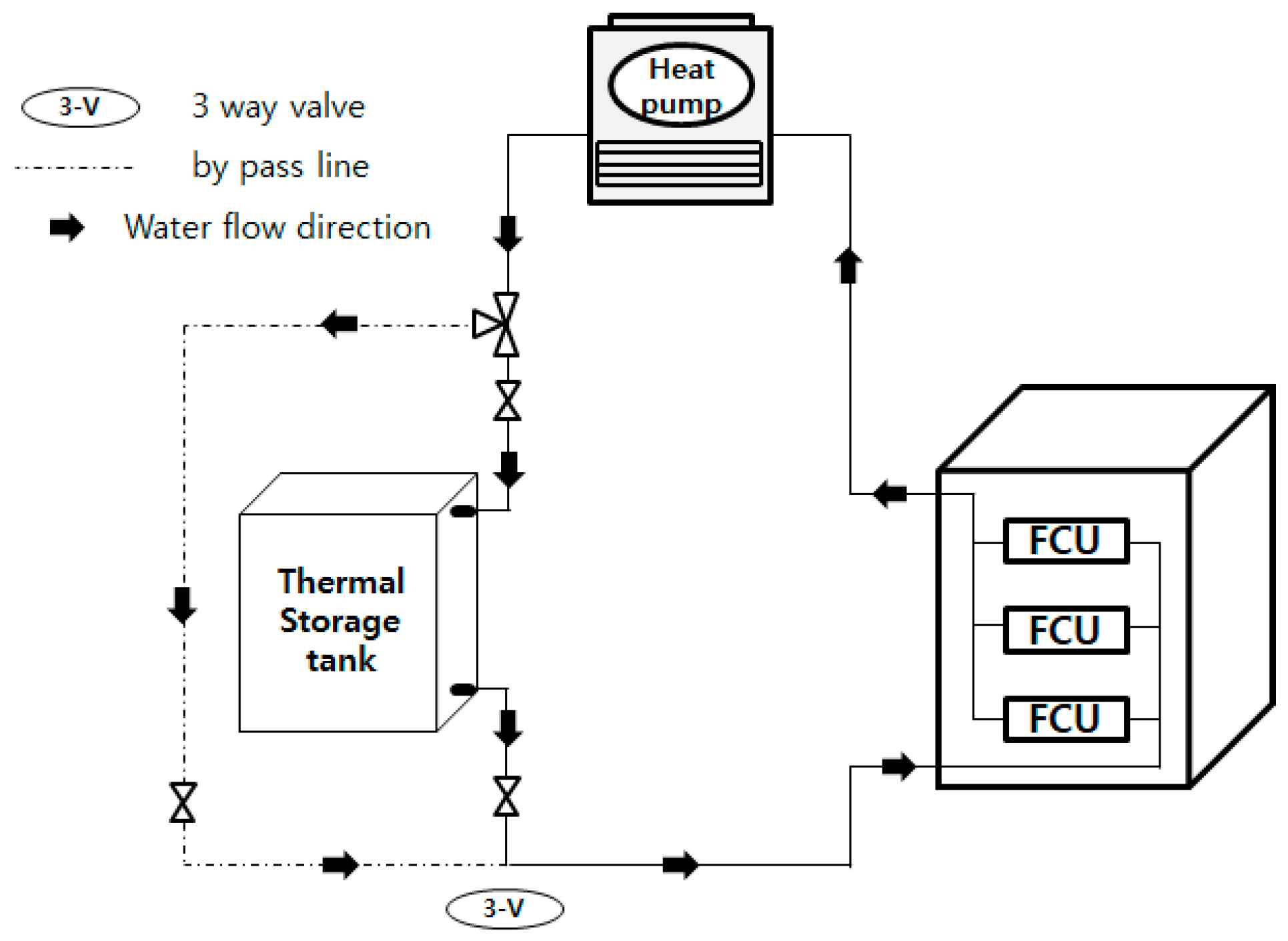
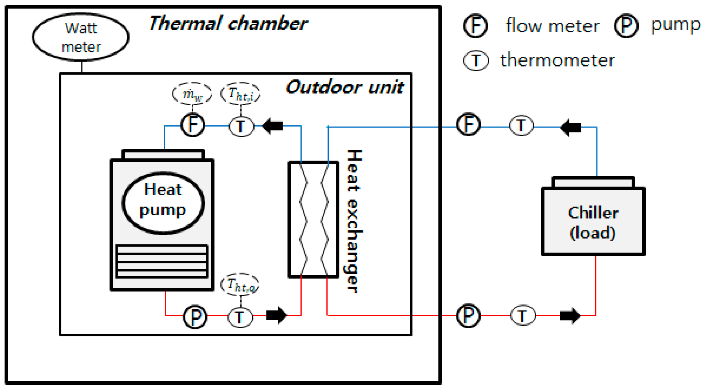
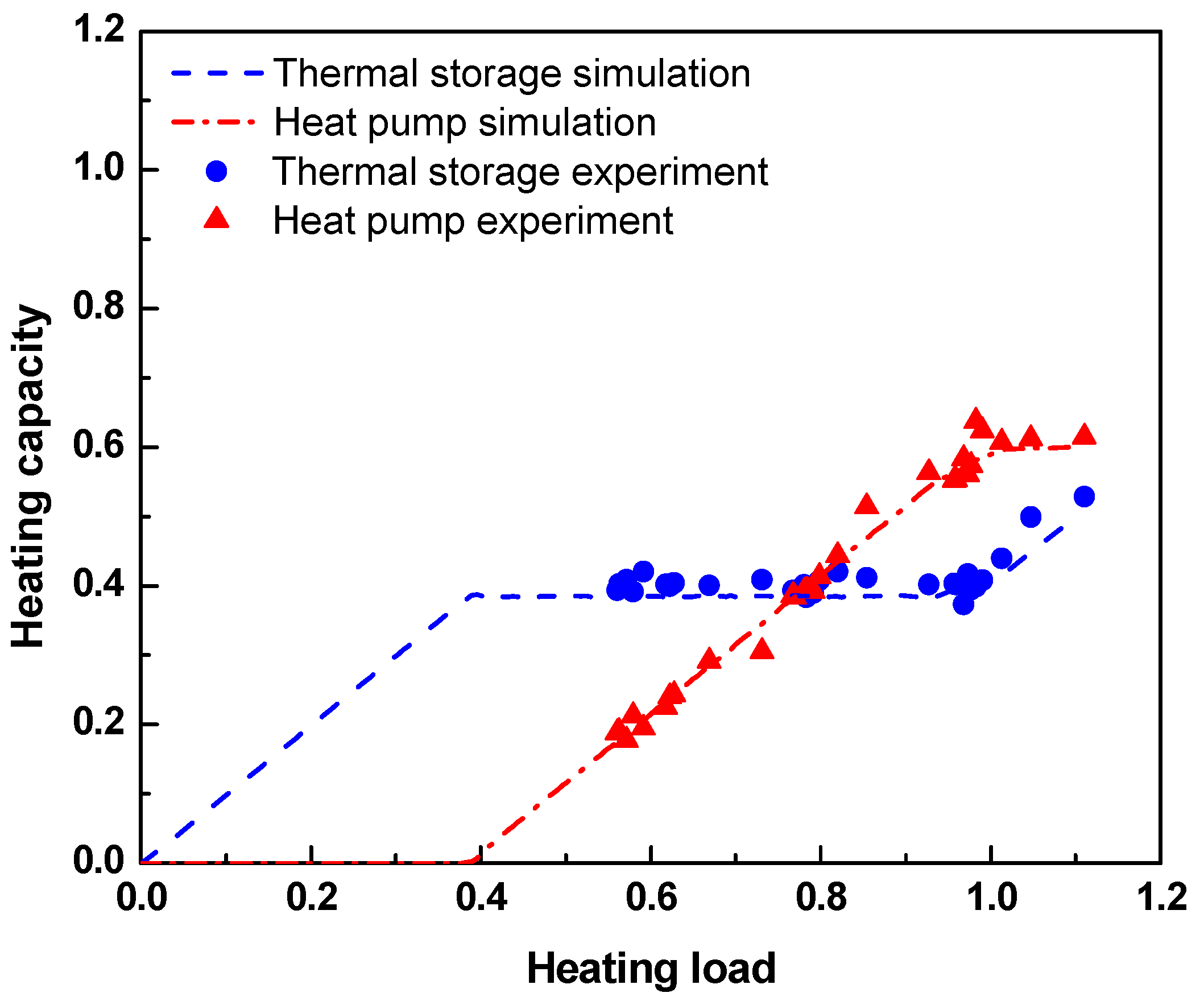
Control simulations were performed under experimental conditions defined section 2.4 to verify the reliability of the simulation results. The virtual load patterns for the experiments were selected using the loads of days that showed 60%, 80%, and 100% of the daily design heating load. Heating load patterns and outdoor air temperatures for three days are derived from TRNSYS using an office building model in Seoul. A chiller is used to provide heating load according to given heating load. To obtain the performance variation of the heat pump by the outdoor temperature change, heat pump is installed in a temperature controlled environmental chamber. Electricity power meter is installed on the heat pump to measure the power consumption. The measurement and control program for the system is developed using LabVIEW (Laboratory virtual instrument engineering workbench). 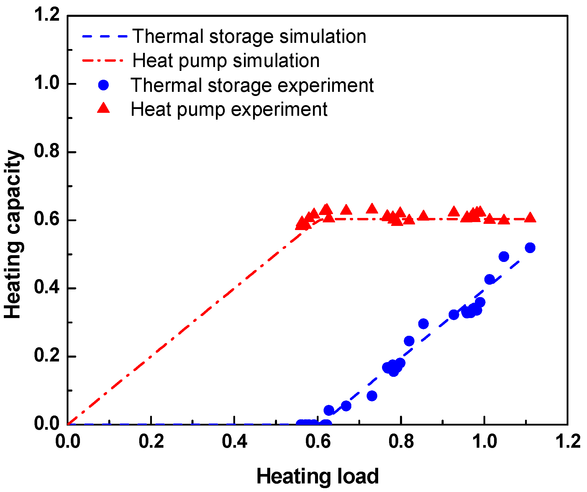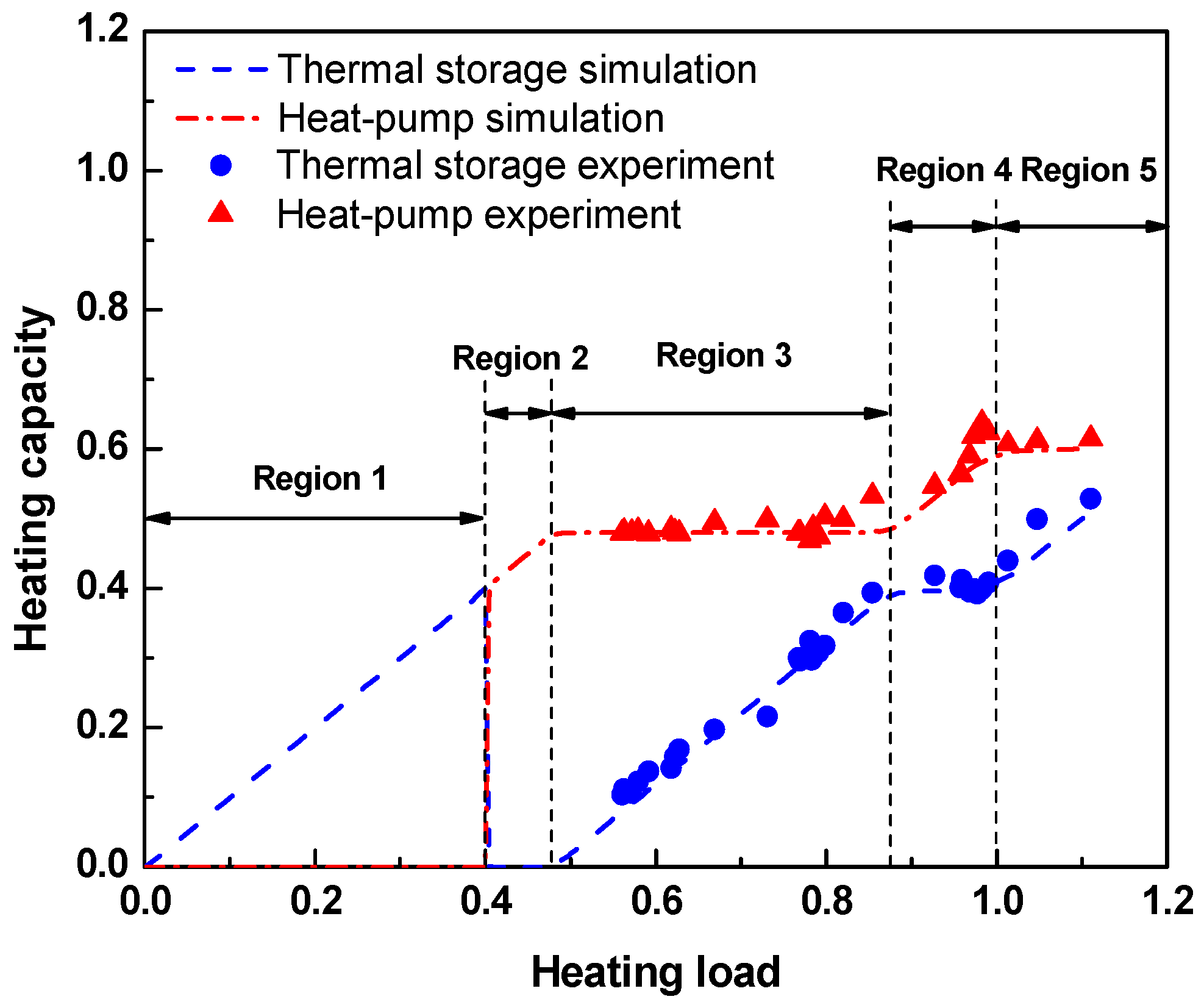The symbols in Figure 10, Figure 11 and Figure 12 represent the comparison of hourly average heat capacity of the thermal storage tank and heat pump of the control methods with results from the simulation model. Experimental data appear as a symbol at about 0.6 or more under the three selected load patterns. Heating capacity of the thermal storage tank and heat pump of the three control methods were found to fit well with previous experimental results.

Table 8. Comparison of simulation results with experiments according to control strategies for various load conditions.

Load	Performance		Experiment			Simulation
			Heat Pump Priority	Thermal Storage Priority	Region Control	Heat Pump Priority	Thermal Storage Priority	Region Control
100%	Heating capacity	Heat pump	0.65	0.61	0.62	0.62	0.60	0.61
		Thermal storage	0.35	0.39	0.38	0.38	0.40	0.39
	Heat pump power consumption	Day	0.6	0.57	0.57	0.56	0.57	0.57
		Night	0.39	0.43	0.41	0.41	0.43	0.41
		Total	0.99	1.00 1	0.98	0.97	1.00 1	0.98
80%	Heating capacity	Heat pump	0.62	0.43	0.49	0.6	0.44	0.48
		Thermal storage	0.19	0.38	0.32	0.21	0.37	0.33
	Heat pump power consumption	Day	0.49	0.37	0.39	0.46	0.38	0.39
		Night	0.15	0.36	0.30	0.16	0.35	0.30
		Total	0.64	0.73	0.69	0.62	0.73	0.69
60%	Heating capacity	Heat pump	0.62	0.26	0.39	0.61	0.23	0.41
		Thermal storage	0	0.36	0.23	0	0.38	0.20
	Heat pump power consumption	Day	0.45	0.25	0.32	0.48	0.24	0.33
		Night	0	0.32	0.16	0	0.35	0.17
		Total	0.45	0.57	0.48	0.48	0.59	0.50

¹ Non-dimensional reference; thermal storage priority method when the heating load 100%.

indicates the comparison between the experiments and simulations in terms of heating capacity of the heat pump and storage tank and power consumption of the heat pump during daytime and nighttime. To compare the results with experimental outcomes, the results from the thermal storage priority method were normalized when the load was 100% of the design heating load. Nighttime power consumption is equal to heat pump’s power consumption required for recharging the amount discharged from tank during daytime.

When load is 100% of design load, experimental results and simulations for all control methods show a heat pump capacity of 0.60–0.65 and thermal storage capacity of 0.35 to 0.40, with differences within 5%. The reason for this similarity is the comparable modes of operation for all control methods, since the heat pump and thermal storage tank operate almost under design conditions, which are 0.6 and 0.4, respectively, as the load approaches 100% of design load. Therefore, in terms of power consumption, the experimental and simulation results show similar values of 0.56–0.60 during daytime and 0.39–0.43 during nighttime.

When the load is 80% of design heating load, each control method generates variations in heating capacity and power consumption due to the different operational characteristics. In both experimental and simulation results, heating capacity of the heat pump is largest in the heat pump priority method, followed by the region control method and thermal storage priority method, whereas that of the thermal storage tank shows the reverse. The heating capacity values obtained experimentally and via simulations showed high consistency, with differences within 0.02. It is expected that daytime and nighttime power consumption are proportional to heating capacity of the heat pump and thermal storage tank, but COP of the heat pump affects practical power consumption. Indeed, total power consumption is lowest in the heat pump priority method, which is expected to operate the highest part load ratio of the heat pump. However, nighttime power consumption, which experiences relatively inexpensive rates, was the largest in the thermal storage priority method, while the region control method lay in the middle of the other methods in terms of power consumption. The simulation results coincide well with the experimental results, with excellent pattern prediction.

When the load is 60% of design heating load, the heat pump priority method controls the heat pump to meet the load entirely on its own. In the thermal storage priority method, heating capacity of the thermal storage tank is the highest at 0.36, while that of the heat pump decreases as the load falls. Overall power consumption of this method is larger than those of the other two methods, as PLR of the heat pump falls. When the load is 80% and 60% of design load, the heat pump operates at full load under the heat pump priority method, as opposed to at its optimum heating capacity under the region control method; however, under the thermal storage priority method, the heat pump operates at lower PLR, as the load decreases to meet heating load.

3.2. Winter Simulation Results

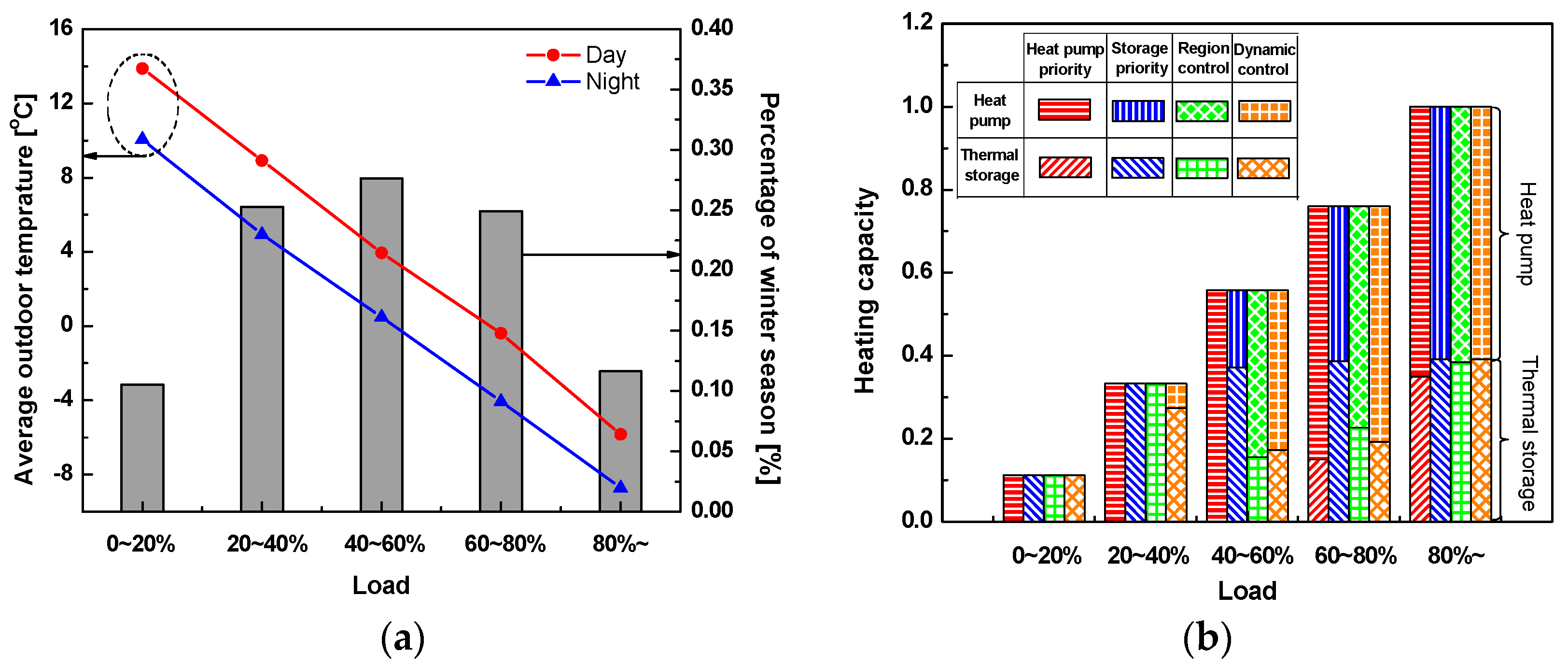
Control performance simulations are performed during winter using the heat pump priority method, thermal storage priority method, region control method, and dynamic programming method. Figure 14a shows the frequency ratio of heating load against design heating load in winter, along with daytime and nighttime daily average outdoor temperatures at a specific load. Heating load during winter shows a higher frequency at 20–80% of design load, and the number of days with low load (0–20%) or high load (>80%) are relatively few. Heating load tends to rise as outdoor temperature decreases. Given that daytime load is the same, the nighttime outdoor temperature is 3.8 °C lower than its daytime counterpart.

Figure 14b indicates the simulation results for control methods based on the heating load throughout winter. When the heat pump priority method is used, the heat pump handles entire heating load when it is 60% or less. When it exceeds 60%, the thermal storage tank increases heating capacity to handle the load, as the heat pump cannot increase its capacity any further. In the thermal storage priority method, heating capacity of thermal storage is fixed at 0.4 when the load is 40% or more; otherwise, entire heating load is handled by the thermal storage tank. The region control method shows a pattern similar to that of the thermal storage priority method when the heating load is 40% or less. When the load exceeds 40%, the heat pump does operate, but with a capacity lower than that of the heat pump priority method where the heat pump operates at full capacity. 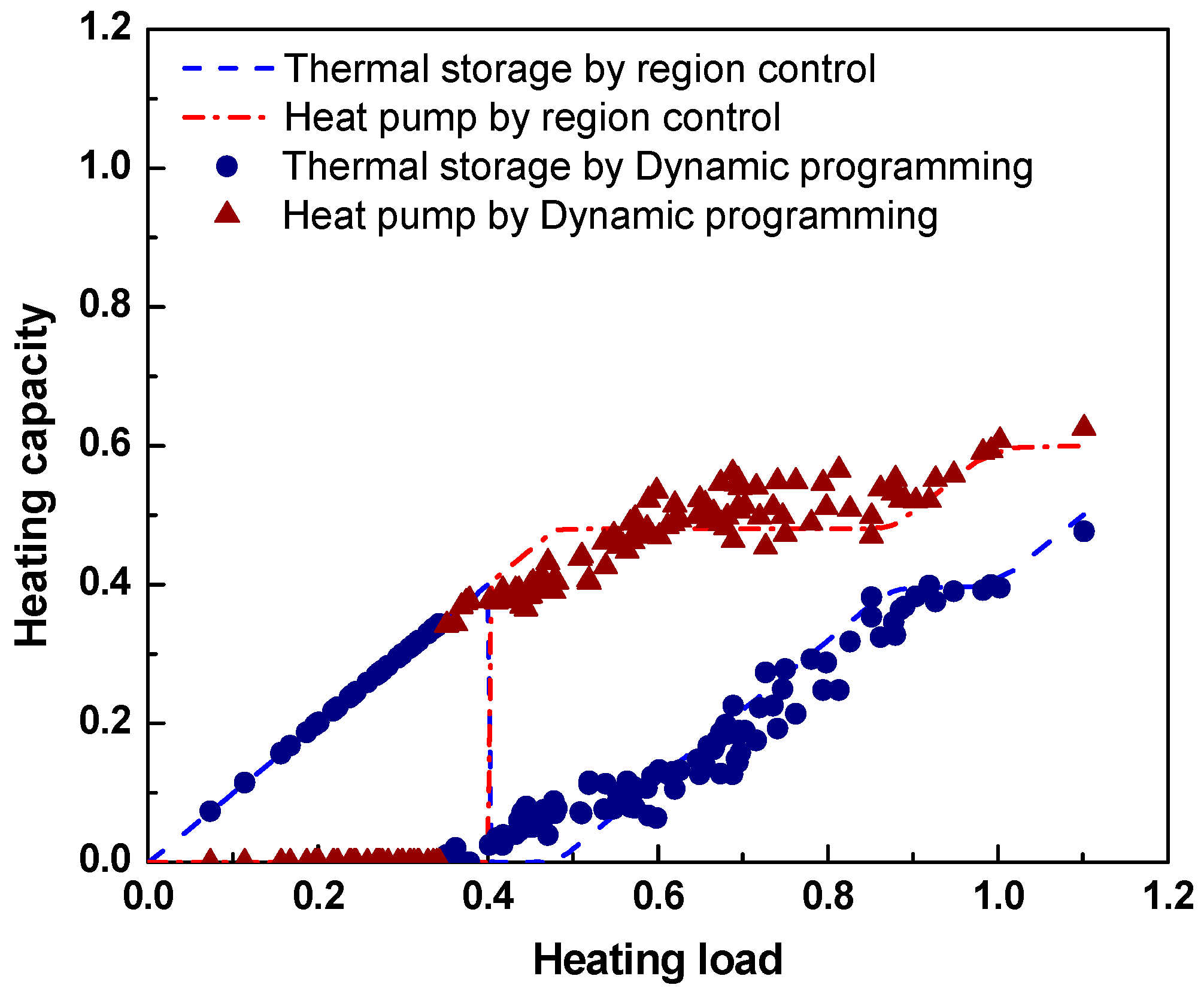As indicated in Figure 12, the heat pump is operated at optimal PLR for heating load of 0.48–0.88, distinguishing this method from the heat pump priority method with a full-load heat pump. In the dynamic programming method, the thermal storage tank handles most of the load when it is less than 40%. For load over 40%, heating capacity of the heat pump becomes larger than that of the thermal storage tank. Unlike the region control method, the dynamic programming method does not divide the control area with respect to load size, but follows the minimum cost path. Nevertheless, Figure 13 shows similar patterns arising from the two methods.

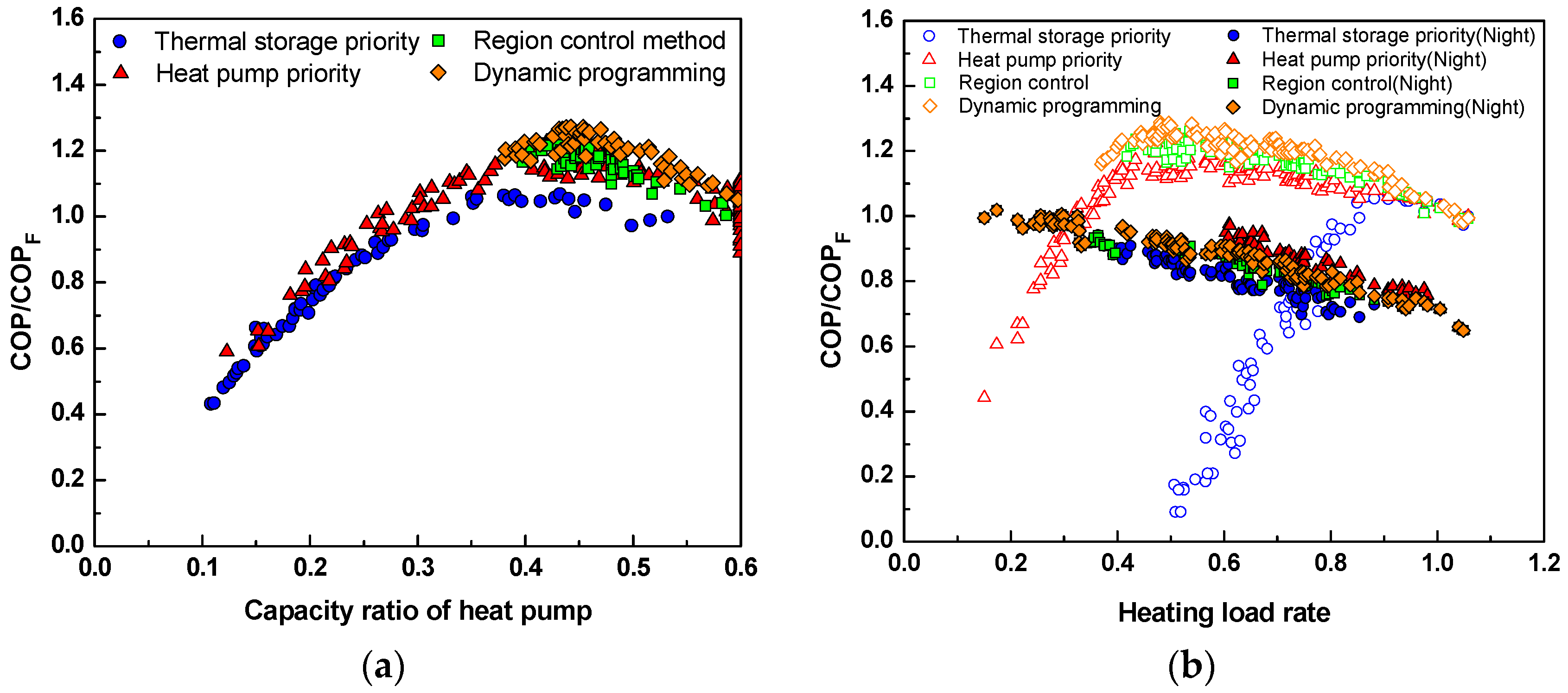
Power consumption to generate heating capacity of the heat pump with control methods is closely related to COP of the heat pump. The heat pump’s COP against its heating capacity is shown in Figure 15a. The heating capacity is divided by design load for normalization. COP increases with heating capacity, as displayed in Figure 7b, and reaches a peak when heating load is 0.48, which is equivalent to PLR of 0.8. COP varies depending on the control method, even when heating capacity is identical, because the heat pump has different operating conditions for each control method.

In the thermal storage priority method, the thermal storage tank handles the heating load first, and the rest is handled by the heat pump as the load rises. Therefore, the heat pump operates when the load is relatively larger compared to the other methods. Large heating loads mean low outdoor temperatures, which leads to low COP of the heat pump with this method, even when the heat pump capacity is identical. In the heat pump priority method, the heat pump operates when the outdoor temperature is high and the load is small, so COP is higher than in the thermal storage priority method and full-load operation is frequent. The heat pump in the region control method operates only in the regions with large heating capacity due to its control characteristics. The dynamic programming method is expected to minimize power consumption and shows the highest COP of the heat pump under the same heating capacity conditions.

Figure 15b shows COP of the heat pump when different control methods are selected to respond to different levels of heating load. During nighttime, the heat pump charges an amount of heat equal to that discharged from the storage tank during daytime. COP distribution of the heat pump at night is also shown. COP of the heat pump depends on outdoor temperature, heating capacity, and outlet water temperature, and the performance varies in accordance with operational characteristics of the heat pump, which is governed by a control method to meet the heating load.

When the load is low, at a level of 0.4 or less, the heat pump priority method uses the heat pump solely. COP is low because PLR is small. When the load is higher than 0.4, heating capacity of the heat pump increases with high COP in all methods except the thermal storage priority method. However, in terms of daytime COP, the region control method with optimal PLR and the dynamic programming method with minimum cost path are found to be superior to the heat pump priority method at full load.

COP is lowest in the thermal storage priority method, because the heat pump begins operating from the heating load of 0.4 and continues operating with small PLR despite large heating load. When the load increases to 0.88 or more, the operational conditions are close to design load; therefore, the control methods show high PLRs and thus similar COPs.

At night, the heat pump operates at full load to charge an amount of heat equal to that discharged from the thermal storage during daytime. Therefore, COP is higher than during daytime with low PLR. Nonetheless, as presented in Figure 14a, outdoor temperatures are lower at night than during the day, and hence, nighttime COP is lower than daytime COP with a high PLR.

Large heating load indicates that the outdoor temperature is low, during which time nighttime COP of the heat pump decreases. In contrast, when the heating load is 0.4 or less, nighttime COP does not vary significantly depending on the control method, except in the heat pump priority method, as only the thermal storage tank handles heating load. When heating load is between 0.4 and 0.88, nighttime COP is lowest in the thermal storage priority method; this is because nighttime charging operation takes longer as the discharged amount is larger in the thermal storage tank. In winter, the outdoor temperature declines as the night progresses, decreasing performance of the heat pump operating at night. For the same reason, nighttime COP is higher in the heat pump priority method, which uses the thermal energy tank in thermal storage less and thus operates the heat pump for a shorter period at night. Nighttime COP for the region control and dynamic programming methods are lower and higher than those for the heat pump priority and thermal storage priority methods, respectively. When nighttime heating load exceeds 0.88, nighttime COPs of all control methods converge to design specifications.

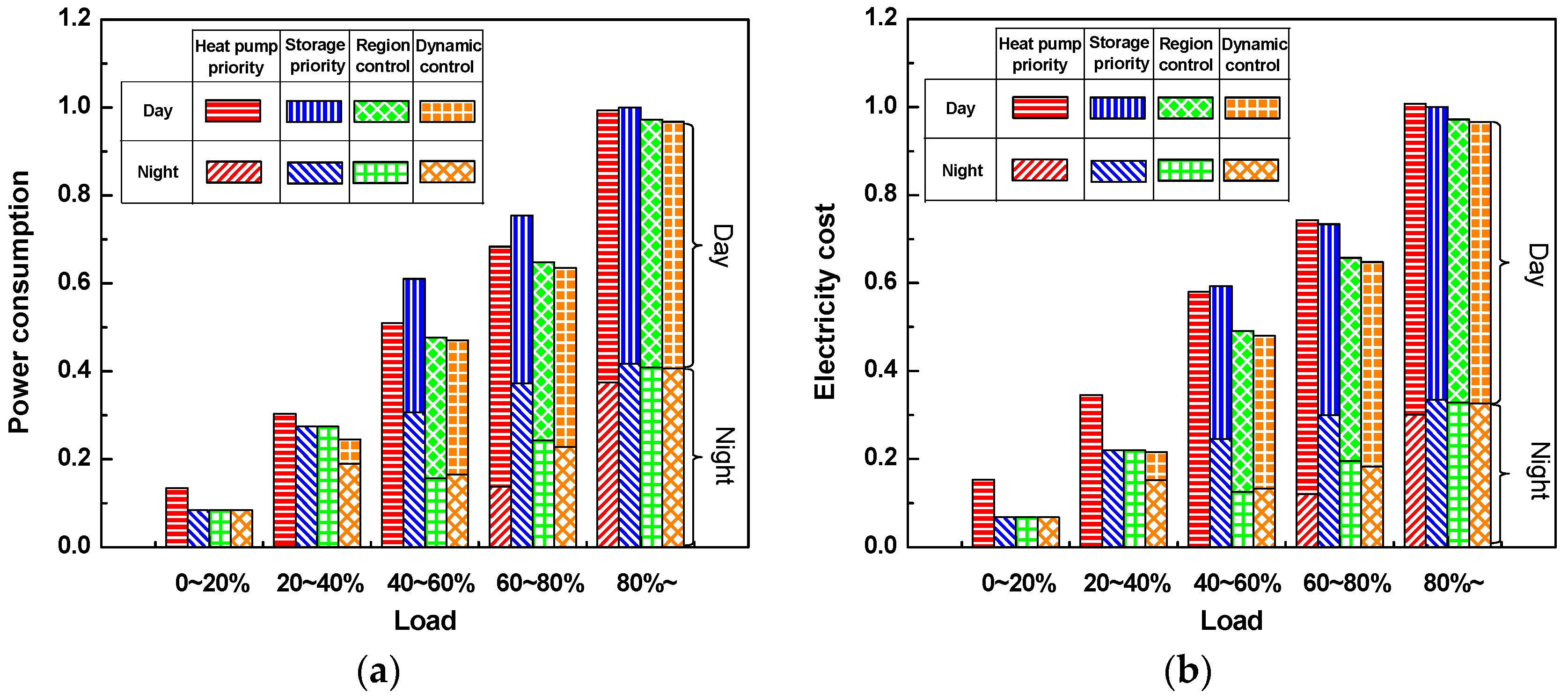
Figure 16a,b shows daily average power consumption and electricity cost according to heating load during winter, respectively. These values are demonstrated non-dimensionally based on the thermal storage priority method when the heating load is 80% or more. The upper portion of the bars indicate power consumption and electricity cost of the heat pump during daytime, while the bottom portion refers to those during nighttime.

When heating load is small (0–40%), the thermal storage tank handles the entire load in the thermal storage priority and region control methods. Therefore, same amount of power is consumed at night in both cases. In the heat pump priority method, the heat pump alone carries the heating load with low PLR. As indicated in Figure 15b, COP is lower during daytime than nighttime when load is small, so power consumption is higher in the heat pump priority method. In the dynamic programming method, the thermal storage tank handles most of the load, so power consumption is lowest, albeit by a narrow margin.

In medium-load range (40–80%), the thermal storage tank and heat pump carry the heating load simultaneously in the thermal storage priority method, and the heat pump capacity increases with load size. This method shows the greatest power consumption due to the lowest COPs both during the night and day. The heat pump priority method has lower daytime COP due to full-load operation than the region control and dynamic programming methods, but has the lowest power consumption because the charging thermal energy is small during nighttime, when COP is low. In the region control and dynamic programming methods, the heat pump charges less thermal energy at night than in the thermal storage priority method, but more than in the heat pump priority method. These advanced methods operate the heat pump more than the heat pump priority method in the medium-load range, but their high daytime COP tends to reduce total power consumption. Further, the dynamic programming method has better daytime COP than the region control method, which explains its lowest power consumption level.

When heating load is high (>80%), the thermal storage priority method shows a slightly higher level of power consumption than the heat pump priority method, since COP of the heat pump is lower at night than during the day. The region control and dynamic programming methods show slightly lower power consumption than the heat pump priority method. The heat pump priority method operates the heat pump at full load, but, as Figure 15b indicates, the region control and dynamic programming methods operate the heat pump with better COP during daytime than that of the heat pump priority method. As heating load increases, operational conditions of the heat pump and the thermal storage tank become similar to design conditions, which eliminates operational differences among the control methods.

It was confirmed that power consumption in the region control and dynamic programming methods was lesser than that in the conventional methods, and it decreased further in the medium-load range, which occurs most frequently. This is because conventional methods operate the heat pump either at full load or low PLRs, while the advanced methods operate it in the highly efficient medium-load range, resulting in reduced power consumption.

Based on information presented in Table 6, the nighttime rates are cheaper than the daytime rates. Therefore, if the total power consumption is the same, the electricity cost is lower when nighttime heating load is higher. In the low-load region, a vast majority of the electricity used in each control method is consumed during either daytime or nighttime. The heat pump priority method results in high power consumption and the electricity costs are dramatically higher than those in other methods because it utilizes expensive daytime electricity. The dynamic programming method has the lowest power consumption, but, since it depends partially on daytime electricity, the electricity cost is only slightly less than that in the conventional methods, which primarily use nighttime electricity.

In the medium- and high-load regions, the thermal storage priority method shows the highest power consumption. However, as it relies largely on nighttime electricity for heating load over 0.6, the electricity cost is lower than the heat pump priority method. In contrast, the heat pump priority method shows low overall power consumption, yet results in high electricity costs due to its dependence on daytime operation. The region control method shows higher overall power consumption than the heat pump priority method, but tends to be more economical because it largely utilizes nighttime electricity and has less total power consumption than the thermal storage priority method. The dynamic programming method’s response is similar to that of the region control method, however the electricity costs are the lowest owing to excellent daytime performance and low daytime power consumption.

In the high-load region, the electricity costs are 1.01 for the heat pump priority method, 0.97 for the region control method, and 0.97 for the dynamic programming method. The characteristics of each method become similar as the load increases, resulting in less variation when compared to the low-load range. Accordingly, the region control and dynamic programming methods result in cheaper electricity costs than the heat pump priority method, because they utilize less-expensive nighttime electricity. Compared to the thermal storage priority method, they also have cheaper electricity costs due to the amount saved from high COP of the heat pump during the day and night, and this trend is most remarkable in the medium-load region.

Table 9. Simulation result of winter season according to control methods.

Parameter	Heat Pump Priority	Thermal Storage Priority	Region Control	Optimal Control
Day power consumption	0.77	0.47	0.47	0.49
Night power consumption	0.19	0.53	0.43	0.39
Total power consumption	0.96	1.00 2	0.90	0.88
Electricity cost	1.08	1.00 2	0.92	0.91

² Non-dimensional reference; thermal storage priority method when the winter season.

shows simulation results throughout winter, including daytime and nighttime power consumption and electricity costs by control methods. It is confirmed that the region control and dynamic programming methods are more economical than the conventional methods in terms of electricity costs. The storage utilization and heat pump efficiency have been improved through the region control method, which utilizes optimal PLR of the heat pump, and the dynamic programming method, which explores the minimum cost path. Cheap nighttime rates render these methods highly economical compared to the conventional methods. However, to implement the dynamic programming method in a heat pump–thermal storage system practically, it is necessary to know the heating load pattern in advance, which can be challenging. Therefore, the region control method has an edge over other methods as it is equally economical and can be easily implemented practically.

4. Conclusions

In this study, heating performance simulations during winter (November to March) were performed for a heating system comprising a dual latent thermal storage tank and a heat pump with varying control methods, including the thermal storage priority method, the heat pump priority method, the region control method, and the dynamic programming method. The performance models were developed for the thermal storage tank and heat pump, and the load pattern and outdoor temperature conditions were derived from the standard building load model for the Seoul region in winter using TRNSYS. Using these models, heating capacity, COP, and power consumption of the heat pump were analyzed with different control methods during daytime and nighttime and electricity costs were identified based on electricity rates.

The thermal storage priority method showed high electricity costs because daytime COP of the heat pump was low, resulting in high power consumption. The electricity cost was also high for the heat pump priority method, as the thermal energy tank in storage was used less and the heat pump operated mostly during the day when electricity is costly. By contrast, the region control method reduced electricity costs since it allowed the heat pump to operate under optimal operational conditions. The dynamic programming method was also economical owing to its ability to follow the minimum cost path. Both advanced control methods exploited more of the thermal storage priority method than the heat pump priority method did and were more economical because they had higher COPs than the thermal storage priority method. This trend was most notable in the medium-load region. The total electricity cost for standard office building in Seoul during winter season was compared according to control methods, and it was found that the dynamic programming method can reduce electricity cost by 17% compared to the heat pump priority method and 9% compared to the thermal storage priority method. As the results confirmed, the advanced control methods, i.e., the region control method and the dynamic programming method, resulted in similar outcomes in terms of electricity costs, suggesting that they are remarkably economical in comparison to the conventional control methods.

References

1. Kim, M.-H.; Lee, D.-W.; Yun, R.; Heo, J. Operational Energy Saving Potential of Thermal Effluent Source Heat Pump System for Greenhouse Heating in Jeju. Int. J. Air-Cond. Refrig. 2017, 25, 1750018. [Google Scholar] [CrossRef]
2. Amoabeng, K.O.; Choi, J.M. Review on Cooling System Energy Consumption in Internet Data Centers. Int. J. Air-Cond. Refrig. 2016, 24, 1630008. [Google Scholar] [CrossRef]
3. Baeten, B.; Rogiers, F.; Helsen, L. Reduction of heat pump induced peak electricity use and required generation capacity through thermal energy storage and demand response. Appl. Energy 2017, 195, 184–195. [Google Scholar] [CrossRef]
4. Miara, M.; Günther, D.; Langner, R.; Helmling, S. The outcomes and lessons learned from the wide-scale monitoring campaign of heat pumps in family dwellings in Germany. In Proceedings of the 11th IEA Heat Pump Conference, Montreal, QC, Canada, 12–16 May 2014. [Google Scholar]
5. Air Conditioning and Heating Facility with Thermal Energy Storage, Midnight-Electricity Equipment Technical Specifications, Korea Electric Power Corporation. Available online: https://home.kepco.co.kr/kepco/cmmn/fms/FileDown.do?atchFileId=FILE_000000021208041&fileSn=0 (accessed on 29 November 2017).
6. Mavrigiannaki, A.; Ampatzib, E. Latent heat storage in building elements: A systematic review on properties and contextual performance factors. Renew. Sustain. Energy Rev. 2016, 60, 852–866. [Google Scholar] [CrossRef]
7. Kim, K.-H.; Yoon, Y.-H.; Kim, Y.-K. Experiment on the charging and discharging processes of a closed ice-thermal-energy-storage system. J. Energy Eng. 2007, 16, 164–169. [Google Scholar]
8. Yang, L.; Zhang, X.-S. Performance of a new packed bed using stratified phase change capsules. Int. J. Low-Carbon Technol. 2012, 7, 208–214. [Google Scholar] [CrossRef]
9. Lee, Y.T.; Chung, J.D.; Park, H.J. A numerical study on the discharging performance of a packing module in a thermal storage tank. Trans. Korean Soc. Mech. Eng. B 2015, 39, 625–631. [Google Scholar] [CrossRef]
10. Miara, M.; Günther, D.; Langner, R.; Helmling, S.; Wapler, J. 10 years of heat pumps monitoring in Germany. Outcomes of several monitoring campaigns. From low-energy houses to un-retrofitted single-family dwellings. In Proceedings of the 12th IEA Heat Pump Conference, Rotterdam, The Netherlands, 15–18 May 2017. [Google Scholar]
11. Carey, C.W.; Mitchell, J.W.; Beckman, W.A. The Control of Ice-Storage Systems. ASHRAE Trans. 1995, 101, 1345–1352. [Google Scholar]
12. Ahn, Y.H.; Kang, B.H.; Kim, S.; Lee, D.Y. The operation characteristics and cost analysis of an ice thermal storage system. Korean J. Air-Cond. Refrig. Eng. 2005, 17, 156–164. [Google Scholar]
13. Spethmann, D.H. Application considerations in optimal control of cool storage. ASHRAE Trans. 1993, 99, 1009–1015. [Google Scholar]
14. Braun, J.E. A comparison of chiller-priority, storage priority, and optimal control of an ice-storage system. ASHRAE Trans. 1992, 98, 893–902. [Google Scholar]
15. Kintner-Meyer, M.; Emery, A.F. Cost optimal analysis and load shifting potentials of cold storage equipment. ASHRAE Trans. 1995, 101, 539–548. [Google Scholar]
16. Jung, S.H.; Lee, D.Y.; Kang, B.H.; Kim, W.S. Control strategy for economic operation of an ice-storage system considering cooling load variation. Korean J. Air-Cond. Refrig. Eng. 1999, 12, 140–149. [Google Scholar]
17. Chen, H.-J.; Wang, D.W.P.; Chen, S.L. Optimization of an ice-storage air conditioning system using dynamic programming method. Appl. Therm. Eng. 2005, 25, 461–472. [Google Scholar] [CrossRef]
18. Chang, Y.C. An Outstanding Method for Saving Energy-Optimal Chiller Operation. IEEE Trans. Energy Convers. 2006, 21, 527–532. [Google Scholar] [CrossRef]
19. Henze, G.P.; Biffar, B.; Kohn, D.; Becker, M.P. Optimal design and operation of a thermal storage system for a chilled water plant serving pharmaceutical buildings. Energy Build. 2008, 40, 1004–1019. [Google Scholar] [CrossRef]
20. Kirk, H.D.; Braun, J.E. Development and evaluation of a rule-based control strategy for ice storage system. HVAC&R Res. 1996, 2, 312–334. [Google Scholar]
21. Lee, K.H.; Choi, B.Y.; Lee, S.R. An evaluation of chiller control strategy in ice storage system for cost-saving operation. Korean J. Air-Cond. Refrig. Eng. 2008, 20, 97–105. [Google Scholar]
22. Ice Storage Systems. One of the Systems Series, A Trane Air Conditioning Clinic. TRANE. Available online: http://www.tga-optimierung.de/kaeltetechnik/wp-content/uploads/sites/2/2015/07/Ice-Storage-Systems.pdf (accessed on 24 August 2012).
23. Rachedi, K.; Korti, A.I.N. Computational investigation of thermal interaction phenomena between two adjacent spheres filed with different Phase Change Materials (PCMs). Int. J. Air-Cond. Refrig. 2017, 25, 1750033. [Google Scholar] [CrossRef]
24. Felix Regin, A.; Solanki, S.C.; Saini, J.S. An analysis of a packed bed latent heat thermal energy storage system using PCM capsules: Numerical investigation. Renew. Energy 2009, 34, 1765–1773. [Google Scholar] [CrossRef]
25. Lee, C.S. A Study on Optimal Control Methods for Cooling of Heat Pump and Latent Heat Storage System. Ph.D. Thesis, Department of Mechanical Engineering, Kookmin University, Seoul, Korea, 2015. [Google Scholar]
26. MATLAB. Mathworks 2016. Available online: https://www.mathworks.com/company/events/conferences.html (accessed on 21 May 2016).
27. Kim, D.J.; Jung, W.S.; Chang, Y.S.; Kang, B.H. Heating performance analysis of the region control method for heat pump with thermal storage system. J. Mech. Sci. Technol. 2017, 31, 5569–5579. [Google Scholar] [CrossRef]
28. Arnold, D. Dynamic Simulation of Encapsulated Ice Tanks: Part I—The Model. ASHRAE Trans. 1990, 96, 1103–1110. [Google Scholar]
29. Salvalai, G. Implementation and validation of simplified heat pump model in IDA-ICE energy simulation environment. Energy Build. 2012, 49, 132–141. [Google Scholar] [CrossRef]
30. Cuong, L.N.; Oh, J.-T. The Comparison of Experiment Results and CFD Simulation in the Heat Pump System Using Thermobank and Two-Phase Ejector for Heating Room and Cold Storage. Int. J. Air-Cond. Refrig. 2016, 24, 1650004. [Google Scholar] [CrossRef]
31. Byrne, P.; Miriel, J.; Lenat, Y. Modelling and simulation of a heat pump for simultaneous heating and cooling. Build. Simul. 2012, 5, 219–232. [Google Scholar] [CrossRef] [Green Version]
32. Seok, H.T.; Kim, K.W. Thermal performance evaluation of design parameters and development of load prediction equations of office buildings. Korean J. Air-Cond. Refrig. Eng. 2001, 13, 914–921. [Google Scholar]
33. KSES. Korean Standard Weather Data; The Korean Solar Energy Society: Seoul, Korea, 2013. [Google Scholar]
34. Korea Electric Power Corporation. KEPCO Selective Terms of Supply; KEPCO: Naju, Korea, 2013. [Google Scholar]
Figure 1. Heat pump with thermal storage tank.
Energies 10 02020 g001
Figure 2. PCM (Phase change material) samples and thermal storage tank schematic for heating system: (a) picture of packed PCMs for cooling and heating (left: cooling; right: heating); and (b) schematic of thermal storage tank.
Energies 10 02020 g002
Figure 3. Heat transfer model for thermal storage.
Energies 10 02020 g003
Figure 4. Comparison between the experiment and the simulation results of heat charging process and heat discharging process for 10 h.
Energies 10 02020 g004
Figure 5. Comparison between the experiment and the simulation results: (a) comparison of time step in 5 h instant of charging process; and (b) comparison of control volume layers in 5 h instant of charging process.
Energies 10 02020 g005
Figure 6. Schematic of heat pump performance test.
Energies 10 02020 g006
Figure 7. Performance of heat pump according to PLR (Part load ratio): (a) correction factor models for power consumption of heat pump under part load operation; and (b) the normalized COP (Coefficient of performance) of heat pump according to part load ratio.
Energies 10 02020 g007
Figure 8. Comparison of predicted and measured normalized power consumption of the heat pump.
Energies 10 02020 g008
Figure 9. Conceptual diagram of conventional control methods: (a) thermal storage priority method; and (b) heat pump priority method.
Energies 10 02020 g009
Figure 10. Thermal storage tank and heat pump capacity ratio by thermal storage priority method.
Energies 10 02020 g010
Figure 11. Thermal storage tank and heat pump capacity ratio by heat pump priority method.
Energies 10 02020 g011
Figure 12. Thermal storage tank and heat pump capacity ratio by region control method.
Energies 10 02020 g012
Figure 13. Comparison of region control method and dynamic programming method simulation results.
Energies 10 02020 g013
Figure 14. Analysis of heating load and heating capacity: (a) percentage of winter season and average outdoor temperature by each heating load; and (b) heating capacity rate due to normalized loads with over 80% load.
Energies 10 02020 g014
Figure 15. Performance analysis by control method: (a) the normalized COP by control mode according to capacity ratio of heat pump; and (b) the normalized COP by control mode according to heating load rate.
Energies 10 02020 g015
Figure 16. Power consumption and electricity cost analysis by control method: (a) normalized power consumption by thermal storage priority method according to load size; and (b) normalized electricity cost by thermal storage priority method according to load size.
Energies 10 02020 g016