A Metaheuristic Approach to the Multi-Objective Unit Commitment Problem Combining Economic and Environmental Criteria ^†

Abstract

We consider a Unit Commitment Problem (UCP) addressing not only the economic objective of minimizing the total production costs—as is done in the standard UCP—but also addressing environmental concerns. Our approach utilizes a multi-objective formulation and includes in the objective function a criterion to minimize the emission of pollutants. Environmental concerns are having a significant impact on the operation of power systems related to the emissions from fossil-fuelled power plants. However, the standard UCP, which minimizes just the total production costs, is inadequate to address environmental concerns. We propose to address the UCP with environmental concerns as a multi-objective problem and use a metaheuristic approach combined with a non-dominated sorting procedure to solve it. The metaheuristic developed is a variant of an evolutionary algorithm, known as Biased Random Key Genetic Algorithm. Computational experiments have been carried out on benchmark problems with up to 100 generation units for a 24 h scheduling horizon. The performance of the method, as well as the quality, diversity and the distribution characteristics of the solutions obtained are analysed. It is shown that the method proposed compares favourably against alternative approaches in most cases analysed.

1. Introduction

The power system generation scheduling is composed of two tasks [1,2]: On the one hand, one must determine the scheduling of the turn-on and turn-off of the thermal generating units; on the other hand, one must also determine the economic dispatch (ED), which assigns the amount of power that should be produced by each on-line unit in order to minimize the total operating cost for a specific time generation horizon. The traditional configuration of this problem, known as the Unit Commitment Problem (UCP), was modified to account for environmental concerns.

During the last decades, the rapid growth in the use of fossil fuels has led to the emission of a large amount of atmospheric pollutants, that are continuously released into the environment. The increased public awareness regarding the harmful effects of atmospheric pollutants on the environment, as well as the tightening of environmental regulations, namely due to the goals imposed by the Kyoto protocol and later by the Paris Agreement [3], have forced power utilities to search for different operational strategies. These new strategies must lead to a reduction in pollution and environmental emissions. Thus, power utilities should look for solutions that in addition to being cost-effective must also be environmentally friendly. The carbon emissions produced by fossil-fueled thermal power plants need also to be minimized. It is necessary to consider these emissions as another objective. Therefore, we are in the presence of a problem with two, usually conflicting objectives.

Current research is directed to handle both objectives simultaneously as competing objectives instead of simplifying the multi-objective nature of the problem by converting it into a single objective problem. The multi-objective version of the UCP has not been the subject of extensive research and most of the works reported in the literature either considers the emissions as constraints [4,5] or transforms the problem into a single objective one, see, e.g., [6,7,8]. A recent review on the use of multi-objective optimization (MOO) in the energy sector, namely in the electricity sector, can be found in [9]. Several methods have been reported in the literature concerning the environmental/economic dispatch problem such as Genetic Algorithms [10,11,12], Differential Evolution Algorithms [13,14], Harmony Search Algorithms [15], Gravitational Search Algorithms [16], Particle Swarm Optimization Algorithms [17,18,19], and Bacterial Foraging Algorithms [20]. These methods fall into the category of metaheuristics, which are optimization methods known to be able to provide good quality solutions within a reasonable computational time (see e.g., [21,22]). Different Multi-objective Optimization Evolutionary Algorithms (MOEA’s), such as Niched Pareto Genetic Algorithm (NPGA) [23], Strength Pareto Evolutionary Algorithm (SPEA) [24] and Non-dominated Sorting Genetic Algorithm (NSGA) [25,26] have been applied to multi-objective problems. Since they use a population of solutions in their search, multiple Pareto-optimal solutions can, in principle, be found in one single run.

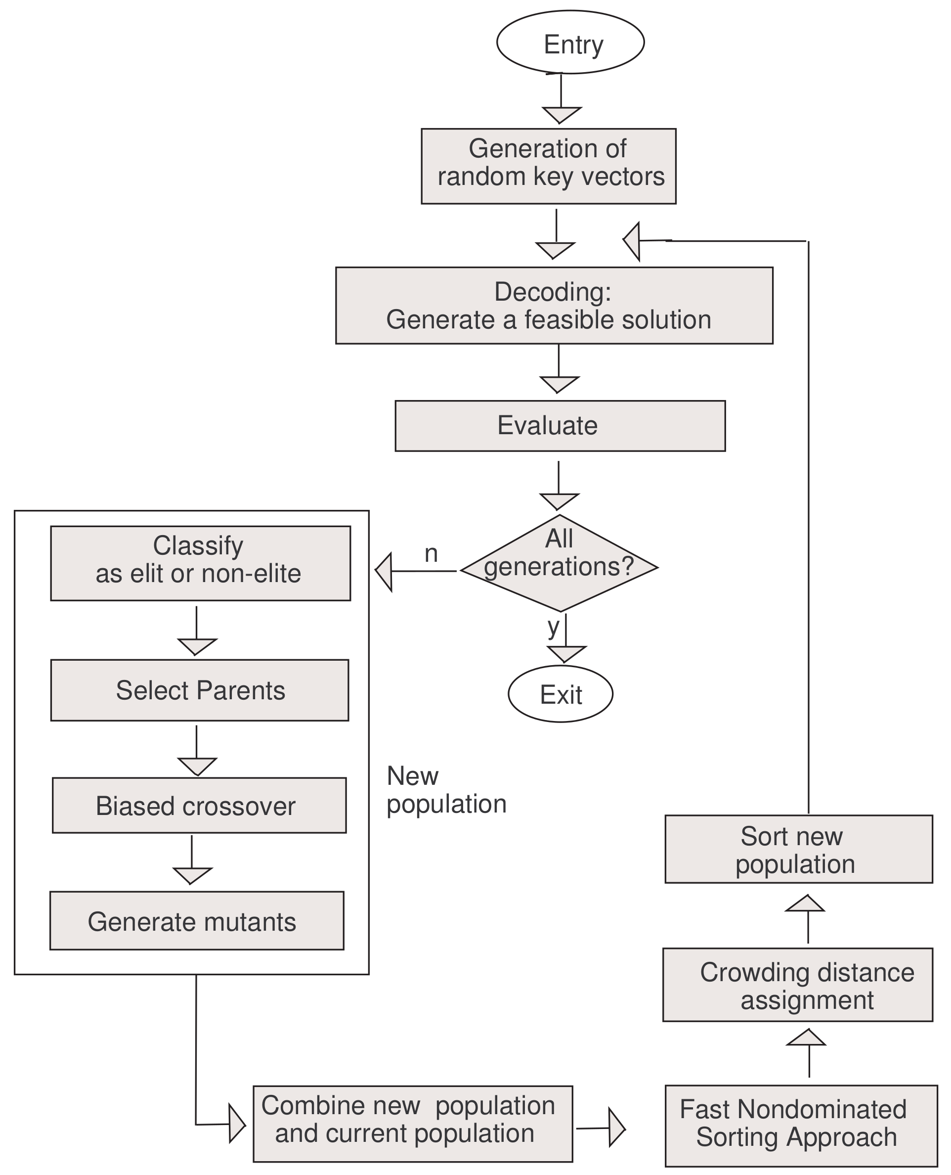
In this paper, we propose to address simultaneously the UC and ED problems using multi-objective optimization. We consider deterministic requirements for the physical generation, load and spinning reserve as is usual in the classical unit commitment problem and, in addition, we take into account the emission of pollutants. The electrical network phenomena such as transmission constraints and power losses are not considered. Also, the uncertainties related to stochastic load demand as well as intermittent power generation by renewable sources such as wind and solar are not considered in our model. A Biased Random Key Genetic Algorithm (BRKGA) combined with a non-dominated sorted procedure and Multi-objective Optimization Evolutionary Algorithm (MOEA) techniques are proposed. 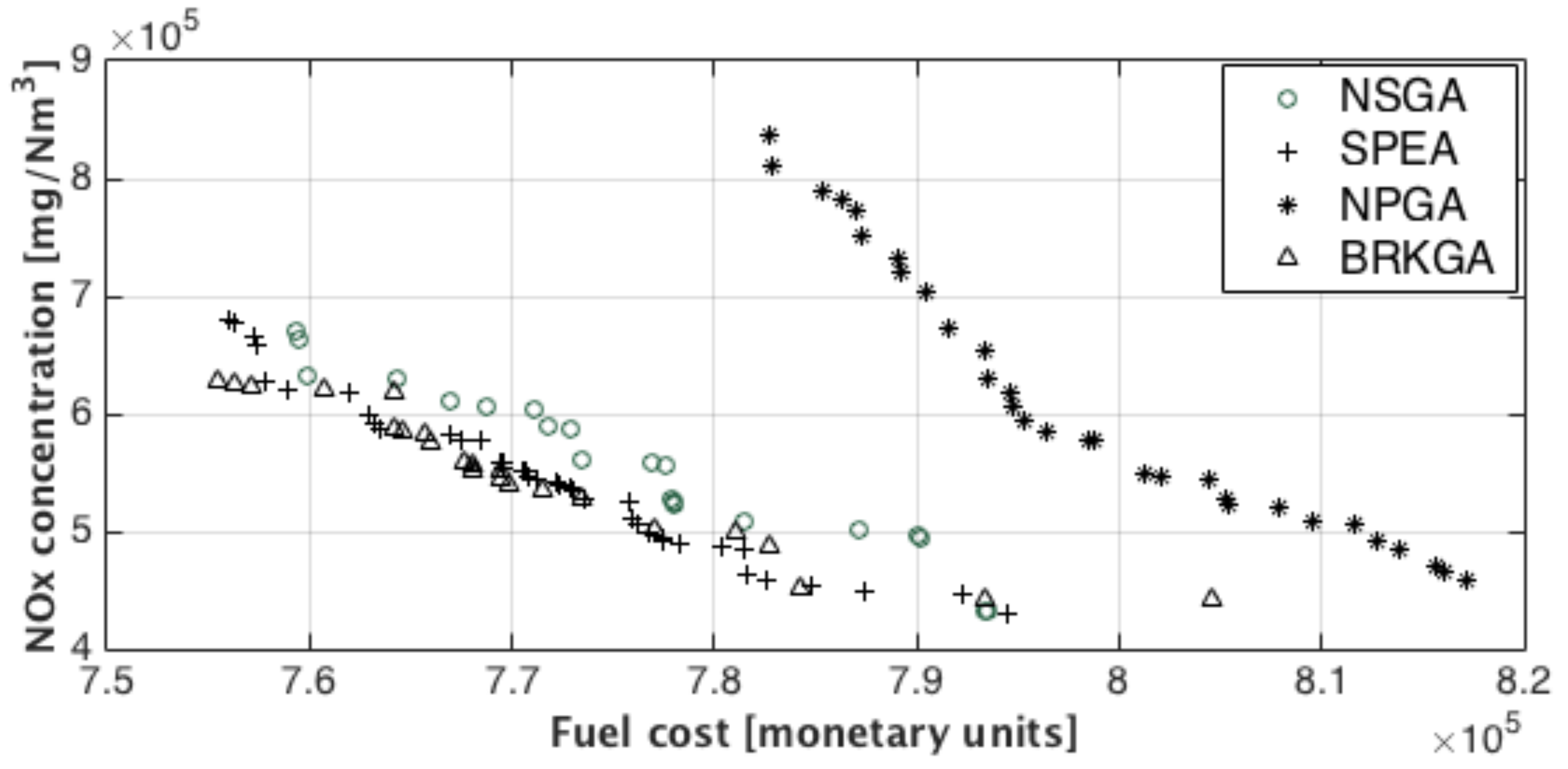The BRKGA developed is based on the framework proposed in [27] and on a previous version developed for the single objective UC problem in [28,29]. Here, the BRKGA approach includes a ranking selection method, that is used for ordering the non-dominated solutions, and a crowded-comparison procedure as in NSGA-II. The crowded-comparison procedure replaces the sharing function procedure used in original NSGA, which allows for maintaining diversity in the population. We also compare the algorithm here proposed with the NSGA-II, SPEA2, and NPGA techniques. Our algorithm is tested on two standard 24-h test systems, introduced in [30,31], each considering several cases involving from 10 up to 100 generating units.

The remaining of the paper is organized as follows. Section 2 surveys the most significant literature on the UCP with environmental concerns. Section 3 provides the description and formulation of the environmental/economic unit commitment problem. An explanation on the BRKGA and alternative solution methodologies as well as their implementation are given in Section 4. In Section 5, the computational experiments are reported and the obtained results discussed. In Section 6 some conclusions are drawn.

2. The Unit Commitment Problem with Environmental Concerns

There exist by now a considerable literature on the UCP including environmental concerns. The environmental concerns have been incorporated into the unit commitment problem in two ways, namely: as a constraint and as an objective. In the latter case, some authors still treat the problem as a single objective problem by combining the two objectives into one, while others address it as a bi-objective problem and thus look for non-dominated solutions.

In some studies, see e.g., [4,5,32,33], the UCP is addressed considering emission constraints. In the aforementioned works, Lagrangian relaxation-based algorithms have been proposed. The authors in [32] propose an augmented Lagrangian relaxation, where the system constraints, e.g., load demand, spinning reserve, transmission capacity and environmental constraints, are relaxed by using Lagrangian multipliers, and quadratic penalty terms associated with system load demand balance are added to the Lagrangian objective function. At each iteration, the quadratic penalty terms are linearized, around the solution obtained at the previous iteration, and the resulting problem is decomposed into N subproblems. The corresponding unit scheduling subproblems are solved using dynamic programming, while the economic dispatch is solved with a network flow algorithm.

A different approach is taken in [5], which uses a modified differential evolution approach. A solution to the UCP is encoded as a binary matrix, representing the switching schedule, and an integer vector, determining the power generated by each unit. After randomly generating the binary matrix, feasibility is ensured for the spinning reserve constraints and for the up/down time constraints by modifying the matrix, if needed. This is done by considering the units in descending order of the ratio of the fuel costs to the maximum power. Then for each time period the power to be generated is randomly obtained for the on units within their generation limits. Once the population has been generated mutation and crossover operators are applied to obtain the next generation. Emissions and power balance constrains are dealt with in the fitness function through the use of heavy penalties. The authors report results for one six-units problem instance with a 24-h planning horizon.

The UCP considering emissions as a second objective function but combined with the main objective function (operating costs) has been addressed by several authors and approaches. In [34] the authors combine the objectives functions using a weighting factor and use a Lagrangian-relaxation-based algorithm. The authors in [35] use a price penalty factor, defined as the ratio between maximum fuel cost and maximum emission of the corresponding generator, to blend the emission with fuel costs. Since the solution procedure proposed relies on an exhaustive enumeration (generates all possible combinations of the generator unit status), it guarantees the optimality of the solution. However, it is only feasible for small sized problem instances (it has been tested on a 5 units system). This problem is also addressed in [36], where the authors propose several techniques, namely: genetic algorithms, evolutionary programming, particle swarm optimization, and differential evolution. Although the authors compare the results obtained with the four techniques, it was not possible to draw any strong conclusions about the techniques efficiency and effectiveness since only two problem instances have been solved. In [37] the UCP with three conflicting functions such as fuel cost, emission and reliability level of the system is considered. These functions are formulated as a single objective function using the fuzzy set theory. A binary real coded Artificial Bee Colony algorithm is proposed, where the binary coded ABC is used to determine the generation units status and the real coded ABC is used to determine the production of the on-line units. The disadvantage of such approaches is that they do not allow for obtaining a set of solutions with a tradeoff between costs and emissions since an apriori compromise is defined. In [38], an approach based on the convex combination of the objective functions, the weighting factor is then varied between 0 and 1. The problem version address only considers constraints on load, spinning reserve, and output limits. The solution procedure is based on the decommitment approach, i.e., it starts by that all units are turned on and then it decommits units one at the time, based on cost savings and on emissions reduction. A single problem instance with 10-units has been solved. This type of approaches has several disadvantages: a uniform spread of weight parameters, in general, does not produce a uniform spread of points on the Pareto-front; Non-convex parts of the Pareto set cannot be reached by minimizing convex combinations of the objective functions; Implies a considerable computational burden since several runs are needed, as many times as the number of desired optimal solutions. Other authors have combined the last two strategies, i.e., combining the two objective functions and imposing constraints on the achievable values for one or both objectives, in order to try to overcome their drawbacks. Catalão et al. [39,40] address the multi-objective unit commitment problem considering cost and emission objective functions. The authors propose an approach based on Lagrangian relaxation, which combines the weighted sum method, using a convex combination of the objective functions, with the $\epsilon$-constraining method, constraining the objectives to be within pre-specified threshold levels. The approach was tested on a case study with 11 thermal units and a scheduling time horizon of 168 h and the results reported demonstrated it to be fast and efficient.

In [6] a Teaching Learning Based Optimization Algorithm (TLBO) is proposed to address the UCP with emissions and costs. In this work, the authors aim is to find a solution that balances the emissions and costs. Thus, they defined as their objective to look for a solution that is about as much far away from the best in both objectives. Therefore, they consider a single objective function, which is given by the weighted sum of the normalized emissions and costs. The TLBO uses a classroom analogy to solve optimization problems. Solutions are students and the solution quality represents the students grade. Solutions (students) interact (learn) with each other and by doing so are capable of improving their quality (grade) by using the best parts of others solutions. The units schedule is represented by a binary matrix that if needed is repaired in order to only deal with feasible solutions. The power generated by each only unit is determined by solving the corresponding quadratic minimization problem. The solutions are then randomly changed to become closer to the best on. Computational experiments were performed by considering the usual benchmark UCP problem instances with 10 up to 100 generating units.

Recent research focus on handling both objectives simultaneously as competing objectives instead of simplifying the multi-objective nature of the problem by converting it into a single objective problem. Several methods have been reported in the literature concerning the environmental/economic dispatch problem such as Genetic Algorithms [10,11,12], Differential Evolution Algorithms [13,14], Harmony Search Algorithms [15], Gravitational Search Algorithms [16], Particle Swarm Optimization Algorithms [17,18,19], and Bacterial Foraging Algorithms [20]. Several MOEAs like Niched Pareto Genetic Algorithm (NPGA) [23], Strength Pareto Evolutionary Algorithm (SPEA) [24] and Non-dominated Sorting Genetic Algorithm (NSGA) [25,26] have been applied to multi-objective problems. Since they use a population of solutions in their search, multiple Pareto-optimal solutions can, in principle, be found in one single run.

In [10] a $ϵ$-defined multi-objective genetic algorithm is described. The proposed algorithm is based on the concept of co-evolution and incorporates a repair procedure that forces the non-linear constraints satisfaction. The non-dominated solutions in archive of finite size are iteratively updated take into account the concept of $ϵ$-dominance. A Multi-Objective Harmony Search (MOHS) algorithm is proposed in [15]. The MOHS algorithm uses a non-dominated sorting and ranking procedure with dynamic crowding distance. In [16] the Opposition-based Gravitational Search Algorithm (OGSA) is used to improve the convergence rate of the Gravitational Search Algorithm. The proposed approach employs opposition-based learning for population initialization and also for generation jumping. The OGSA algorithm was tested on four standard power systems problems of combined economic and emission dispatch (CEED).

Abido [17] propose a multi-objective particle swarm optimization (MOPSO) that includes a hierarchical clustering technique to manage Pareto-optimal set size. The MOPSO performances in terms of non-dominated solutions diversity and well-distribution characteristics are also studied. Zhang et al. [18] propose a new Bare-Bones Multi-Objective Particle Swarm Optimization (BB-MOPSO) algorithm. The BB-MOPSO include a particle updating strategy; a mutation operator with action range varying over time and an approach based on particle diversity to update the global particle leaders. However, the algorithm proposed requires tuning control parameter such as acceleration coefficients, inertia weight, and velocity clamping. Pandit et al. [20] proposes an Improved Bacterial Foraging Algorithm (IBFA) in which a parameter automation strategy and crossover operation is used in micro BFA to improve computational efficiency. The IBFA approach obtains Pareto-optimal solutions for combined static/dynamic environmental economic dispatch. The authors in [26] propose a method combining Non-dominated Sorting Genetic Algorithm-II (NSGA-II) with problem-specific crossover and mutation operators. The initial population is obtained by randomly generating the unit status (binary matrices) except for one solutions that are obtained through a priority list. The power dispatch is obtained by using the lambda-iteration method. Parents are randomly chosen from a pool, formed using binary tournament and the offspring is obtained by applying window crossover. Mutation is applied using swap window and window operators. Then the NSGA-II principle is used to form the next generator. The authors have one problem instance with 60 generating units. This work has then been improved in [41] since problem specific binary genetic operators are used for the unit status matrix (commitment matrix) and real genetic operators are used for the power matrix thus exploring the binary and real spaces separately. The authors also use two different crossover procedures, one to evolve the commitment matrix and another to evolve the power matrix. Solution feasibility concerning to power demand satisfaction is ensured through a repair mechanism. The violation of other constraints results in a violation penalty. Baskar et al. [11] propose a modified NSGA-II (MNSGA-II) algorithm for economic and emission dispatch problem. The NSGA-II drawbacks such as lack of uniform diversity of non-dominated solutions and lack of lateral diversity-preserving operator were corrected by introducing dynamic crowding distance (DCD) and controlled elitism (CE) into the NSGA-II.

There is other research on the UCP that considers renewable energy generating units, which is recent. However, current discussion involves several different issues, such as types of resources [42], uncertainties regarding renewable resources [43,44,45,46], and pumped hydro-energy storage [47,48]. For very recent literature reviews see, e.g., [49,50] and the references therein. Despite these recent research trend, not many works have yet been reported on the MO version of the UCP involving renewable resources, specially without transforming it into a SO version. Here, we refer to the very few and recent exceptions. In [51] a non-dominating backtrack searching algorithm is proposed to approximate the Pareto front regarding cost and risk minimization. The risk objective is related to the possible power shortage and unit outage, due to the consideration of wind generating units and it is modelled as a risk index. Results are provided regarding two problem instances. In [52] a multi-objective gravitational search algorithm (MOGSA) is used to find some Pareto optimal solutions, regarding the minimization of cost and emissions. The UCP considered includes hydro, pump storage, wind farm, and solar farm, with and without ramp rates.

In the next sections, we describe the UCP and ED problems using multi-objective optimization. We also describe the methodology used to solve the problem: a metaheuristic method based on a Biased Random Key Genetic Algorithm and combined with a non-dominated sorted procedure.

3. The Multi-Objective UCP Optimization Based on Evolutionary Algorithms

The problem of scheduling power generators is formulated as a bi-objective optimization model. The problem data is considered deterministic, the uncertainties related to load demand and renewable energy resources (wind, solar) are not studied in this work. Also the electrical network phenomena such as transmission constraints and power losses are not included.

In the multi-objective UC problem, one needs to determine an optimal schedule, which minimizes the production cost and emission of atmospheric pollutants over the scheduled time horizon subject to system and operational constraints. Therefore, the multi-objective UC problem should be formulated including both objectives, i.e., the minimization of the operational costs and the minimization of the pollutant emissions.

$$\mathrm{M}\mathrm{i}\mathrm{n}\mathrm{i}\mathrm{m}\mathrm{i}\mathrm{z}\mathrm{e}\hspace{1em}\left[F(y,u),E(y,u)\right]\phantom{\sum _1^2}$$

(1)

Due to its combinatorial nature, multi-period characteristics, and nonlinearities, the UC problem is a hard optimization problem, which involves both integer and continuous variables and a large set of constraints. The first component of the objective function is concerning to the system operational costs composed of generation and start-up costs.

$$F(y,u)=\sum _{t=1}^T\left(\sum _{j=1}^N\right.\{F_j\left(y_{t,j}\right)·u_{t,j}+S{U}_{t,j}·(1-u_{t-1,j})·u_{t,j}\left.+S{D}_j·(1-u_{t,j})·u_{t-1,j}\}\phantom{\sum _1^2}\right),$$

(2)

where $S_{t,j}$ and $S{D}_{t,j}$ are the start-up and shut-down costs of unit j at time period t, respectively. The generation costs, i.e., the fuel costs, are conventionally given by a quadratic cost functions, $F_j\left(y_{t,j}\right)$, as in Equation (3),

$$F_j\left(y_{t,j}\right)=a_j·{\left(y_{t,j}\right)}^2+b_j·y_{t,j}+c_j,$$

(3)

where $a_j,b_j,c_j$ are the cost coefficients of unit j. On the other hand, the second objective is to minimize the total quantity of atmospheric pollutant emissions such as NO${}_x$ and CO${}_2$.

$$E(y,u)=\sum _{t=1}^T\left(\sum _{j=1}^N\right.\{E_j\left(y_{t,j}\right)·u_{t,j}\left.+S{e}_{t,j}·(1-u_{t-1,j})·u_{t,j}\}\phantom{\sum _1^2}\right),$$

(4)

where $S{e}_j$ is the start-up pollutant emissions of unit j at time period t. Here, $E_j\left(y_{t,j}\right)$ represents the emissions produced by each thermal unit j in on-line status, which is expressed as a quadratic function in terms of output power generation,

$$E_j\left(y_{t,j}\right)={\alpha }_j·{\left(y_{t,j}\right)}^2+{\beta }_j·y_{t,j}+{\gamma }_j,$$

(5)

where ${\alpha }_j,{\beta }_j,{\gamma }_j$ are the emission coefficients of unit j. The constraints can be divided into two categories: the system constraints and the technical constraints. Regarding the first category of constraints it can be further divided into load requirements and spinning reserve requirements, which can be written as follows:

(1)

Power Balance Constraints: The sum of unit generation outputs must cover the total power demand, for each time period.

$$\sum _{j=1}^N{y}_{t,j}·u_{t,j}\ge D_t,t\in \left\{1,2,\dots ,T\right\}.$$

(6)

(2)

Spinning Reserve Constraints: The total amount of real power generation available from on-line units net of their current production level must satisfy a pre-specified percentage of the load demand.

$$\sum _{j=1}^{N}Yma{x}_j·u_{t,j}\ge R_t+D_t,t\in \left\{1,2,\dots ,T\right\}.$$

(7)

The second category of constraints includes unit output range, the minimum number of time periods that the unit must be in each status (on-line and off-line), and the maximum output variation allowed for each unit.

(3)

Unit Output Range Constraints: For each time period t and unit j, the real power output of each generator is restricted by lower and upper limits.

$$Ymi{n}_j·u_{t,j}\le Y_{t,j}\le Yma{x}_j·u_{t,j}.$$

(8)

(4)

Ramp rate Constraints: Due to the thermal stress limitations and mechanical characteristics, the output variation levels of each online unit in two consecutive periods are restricted by ramp rate limits.

$$-{\Delta }_j^{dn}\le y_{t,j}-y_{t-1,j}\le {\Delta }_j^{up}.$$

(9)

(5)

Minimum Uptime/Downtime Constraints: If the unit has already turned on/off, there will be a minimum uptime/downtime time before it is shut-down/started-up, respectively.

$$T_j^{on}\left(t\right)\ge T_{min,j}^{on}\hspace{0.17em}and\hspace{0.17em}{T}_j^{off}\left(t\right)\ge T_{min,j}^{off}.$$

(10)

As already mentioned, the uncertainties related to a varying load demand and varying renewable energy resources are not addressed in this model. Also, the electrical network phenomena such as transmission constraints and power losses are not considered. These assumptions are usual in many studies of the unit commitment problem, as is discussed in works mentioned in the previous section. The main aim of the UCP is to provide a plan for the schedule of units on a relatively long term, typically 24 h or more. After the units are committed and having a plan for the dispatch, the economic dispatch problem is often re-solved using more recent (real-time) data and additional constraints related to the network.

4. Multi-Objective UCP Optimization

In this section, we describe the solution methods to solve the multi-objective UCP optimization, their components, as well as their implementation details. Some performance metrics that are used to evaluate the merits of each method are also discussed.

4.1. Decoding Procedure

The decoding procedure used in all four multi-objective optimization algorithms is the one proposed in [28,29]. For each chromosome, the corresponding solution is obtained in two main stages. Firstly, the output generation level matrix for each unit and time period is computed using the random key values. Each element of the output generation matrix, $y_{t,j}$ is given as the product of the percentage vectors by the periods demand $D_t$, i.e., $y_{t,j}=D_t\frac{R{K}_j}{{\sum }_{i=1}^{N}R{K}_i}$. Here each component of the percentage vectors is given by corresponding random key entry divided by the sum of all random key values as illustrated in algorithm 1 in [28]. Then, the feasibility of the output levels is checked and whenever a constraint is not satisfied the solution is modified by the repair algorithm presented in [29].

4.2. Repair Algorithm

The repair algorithm is composed of several steps. Firstly, the output levels are adjusted in order to satisfy the output range constraints. Next, we have the adjustment of output levels to satisfy ramp rate limits. It follows the repairing of the minimum uptime/downtime constraints violation. Afterwards, the output levels are adjusted in order to satisfy spinning reserve requirements. Finally, the output levels are adjusted for demand requirements satisfaction at each time period. For details on the repairing mechanisms, the reader is referred to [29].

4.3. NSGA II

NSGA II is a fast and elitist non-dominated sorted genetic algorithm [53], which allows to approximating the set of Pareto solution. In this approach, the ranking selection method is used to focus on non-dominated solutions while the crowding distance is computed to ensure diversity along the non-dominated front. The population of size $N_p$ is used for selection, crossover, and mutation to create a new offspring population of equal size. The rank procedure is employed by different levels of domination until all individuals in the intermediate combined population, of size $2N_p$, are ranked. Firstly, the non-dominated solutions are assigned with same rank value and thereafter the crowding distance is computed. The non-dominated solutions must be emphasized more than any other solution. In order to find individuals of the next front, the solutions of the first front are temporarily ignored, and the above procedure is repeated to find subsequent fronts. The individuals of the new population are selected from the intermediate population using subsequent non-dominated fronts in the order of their ranking. To choose exactly the population members, the solutions of the last front are sorted considering the crowding distance by descending order. The NSGA-II approach proposed by [53] was implemented as follows:

• Generate random initial population of size $N_p$, decode individuals, and evaluate solutions;
• Sort the initial population using non-domination-sort. For each individual assign rank and crowding distance;
• For each generation the following steps are performed: Select the parents, which are fit for reproduction by using the binary tournament selection based on the rank and crowding distance; the genetic operators simulated binary crossover and polynomial mutation are applied under selected parents to create the offspring population of size $N_p$ ; the offspring population is combined with parent population (the size of intermediate population is the double); after non-dominated sorting of the combined population, only the best $N_p$ individuals are selected based on its rank and crowding distance; a new generation is then obtained maintaining the population size fixed; the stop criterium is a maximum number of generations previously established.

4.4. NPGA

A Niched Pareto genetic algorithm was presented in [23]. This technique involves the addition of two specialized genetic operators: Pareto domination tournaments and fitness sharing. These operators allow for selection based on a partial ordering of the population, as well as, to preserve diversity in the population. Tournament selection is used to adjust selection pressure by changing the tournament size. Two candidates are chosen at random from the current population. A comparison set of $tdom$ individuals is also chosen randomly. Each of the candidates is compared to each individual in the comparison set. If a candidate is dominated by the comparison set, and other is not, the former loses the competition. If there are tournament ties, i.e., neither or both candidates are dominated by the comparison set, the selection is based on the fitness sharing of individuals, using niche counts as computed for the objective space in [23]; see Equation (11). Each candidate niche count is computed in the objective space, using its evaluated objective values. The candidate with lowest niche count wins the tournament. Tournaments are held until the next generation is filled. The niche count for candidate i is given by:

$$m_i=\left\{\begin{array}{cc}\sum _{j\in Pop}\left(1-\frac{d_{i,j}}{{\sigma }_{share}}\right)\hfill & \mathtt{if}\hspace{0.17em}{d}_{i,j}<{\sigma }_{share}\hfill \\ 0\hfill & \mathtt{if}\hspace{0.17em}{d}_{i,j}>={\sigma }_{share}\hfill \end{array}\right.,$$

(11)

where $d_{i,j}$ is the Euclidean distance between competitor i and other individual j. Here ${\sigma }_{share}$ is the niche radius, i.e., the specified distance. The winner of the tied tournament is the competitor with the lowest niche count. As in [23], the fitness sharing is updated continuously, once the niche counts are calculated using individuals in the partially filled population of the next generation, rather than that of the current generation. Then crossover and mutation operators are applied to the new population.

4.5. SPEA 2

The Strenght Pareto Evolutionary Algorithm (SPEA) was introduced in [24] and an improved version, known as SPEA2 is given in [54]. In this algorithm, non-dominated solutions are stored in an external set. The individuals are assigned according to the Pareto dominance concept. When the non-dominated solutions exceed a previously fixed size for the external set, the number of individuals in the external set is reduced by means of a truncation technique, as in [54]. If the number of non-dominated individuals is less than the predefined external set size, the external set is filled up by dominated individuals. The fitness assignment occurs in two different stages. The individuals are assigned by the strengths of its dominators in both the external set and the population. Strenght represents the number of individuals in the population and in the external set covered by the individual considered. The fitness of each individual is given by the sum of the strengths of its dominators in the external set and in the population. If more than one individual has the same fitness value, the density estimation technique is used as given in SPEA2 [54]. This technique results from an adaptation of the kth nearest neighbor method. The basic idea of the truncation procedure is to remove the individual which has the minimum distance to another individual. If there are several individuals with minimum distance, the individuals with second smallest distances to another individual are removed and so on. The SPEA-II approach proposed by [54] implements the following steps:

Step 1.

Generate the initial population, decode individuals, evaluate solutions, and create the empty external set to keep the Pareto front approximations;

Step 2.

Compute fitness values of individuals in the population and in the external set;

Step 3.

Copy non-dominated individuals of the population to the external set;

Step 4.

Update the external set keeping only the non-dominated solutions. When the number of non-dominated solutions is higher than the specified size for the external set, it is reduced by applying the truncation technique. If the number of non-dominated individuals is less than the external set size, the external set is filled up with dominated individuals;

Step 5.

The algorithm stops when the maximum number of generations is reached;

Step 6.

The mating pool is filled using the binary tournament selection with replacement on the updated external set;

Step 7.

After the recombination of the mating pool, the crossover and mutation operators are applied and a new population is created. Increment the generation counter and repeat from Step 2.

4.6. BRKGA Multi-Objective UC Approach

The BRKGA is adapted using the ranking selection method for ordering the non-dominated solutions according to the Pareto domination concept, while the crowding distance is used to break the ties by choosing the best individuals to be included in new population. Details about the BRKGA approach are given in [27,28]. The initial population, with size $N_p$, is constructed by generating the random keys. Given a population of chromosomes (random keys) the decoding procedure is applied such that to each chromosome corresponds a feasible UC solution. The fitness function used to evaluate the solutions includes both the total operational costs and CO${}_2$ or NO${}_x$ pollutant emissions. We have adopted a fitness procedure similar to that of NSGA-II, given in [53]. Therefore, the population is sorted based on the non-domination concept. Each solution is assigned a fitness (rank) equal to its non-dominated level. The biased selection and biased crossover operators and the introduction of mutants are used to create an offspring population, also of size $N_p$. On the one hand, the biased selection ensures that one of the parents used for mating comes from a subset containing the best solutions of the current population. On the other hand, the biased crossover chooses with higher probability an allele from the best parent. Mutants are generated in the same way as the initially population and are introduced directly in the next generation. We start by combining the current population with the newly obtained one. The combined population size is the double ($2N_p$) of the current population and it is sorted by the non-domination criterion (Fast Non-dominated Sorting Approach). The non-domination criteria leads to several levels of non-dominated fronts. The first level includes all non-dominated individuals of the combined population. The second level contains solutions only dominated by the solutions in the first level. All other levels are defined in a similar way, that is, each level contains only solutions dominated by all previous non-dominated levels. In order to obtain the new population we go through the different levels, in ascending order, and include all its solutions if $N_p$ is not reached; otherwise only some solutions are included, until $N_p$ is reached, using the descending order of crowding distance as a selection criterion. The multi-objective BRKGA approach is illustrated in Figure 1.

4.7. Performance Metrics

Genetic Operators in BRKGA

Biased Selection: a pair of parents are selected from the current population. This population is divided into two sets: The elite set, comprising the best individuals, and the non-elite set, comprising the remaining individuals. One parent is selected from the elite set, while the other parent is chosen from the remaining, non-elite, individuals. Biased Crossover: Given two parents and a specified probability of crossover, the crossover interchanges the genes or alleles to produce a new individual. As already mentioned, genes are chosen by using a biased uniform crossover, that is, for each gene, a biased coin is tossed to decide on which parent the gene is taken from. This way, the offspring inherit the genes from the elite parent with a higher probability (0.7 in our case). Mutants: To ensure diversity and to avoid premature convergence, we introduce a percentage of new individuals, called mutants, in the population. These individuals are randomly generated, as was the case for the initial population.

The solutions of the different MOEAs considered are compared by analyzing the approximated Pareto fronts produced. In addition, four different performance measures are used considering the distinct goals of convergence to the Pareto optimal front and the uniformity of distribution in terms of dispersion and extension. We use the set coverage metric [55]. This metric takes into consideration a pair of non-dominated sets comparing the fraction of each set that is covered by the other set and is defined as

$$Cov(A,B)=\frac{\left|\left\{b\in B;\exists a\in A:a\mathtt{cover}b\right\}\right|}{\left|B\right|},$$

(12)

where $\left|.\right|$ represents the size (cardinality) of a set. If $Cov(A,B)=0$; then none of the points in the set B are covered by the set A. If $Cov(A,B)=1$; then all points in B are dominated by or equal to points in A. It should be noticed that $Cov(A,B)$ is not necessarily equal to $1-Cov(B,A)$.

The contribution measure [56] $Con(A,B)$ of an approximation Pareto front A relatively to another approximation Pareto front B gives the percentage of the solutions of the non-dominated set of $A\cup B$. Thus, this metric value has to be greater than $0.5$ to indicate that A is better than B in terms of convergence of the Pareto front. Let F be the set of solutions in $A\cap B$, $F^{*}$ the set of Pareto solutions of $A\cup B$. Let $D_1$ ($D_2$) be the set of solutions in A (B) that dominate some solutions of B (A) and let also $N_1$ ($N_2$) be the noncomparable solutions of A (B). Therefore, the contribution measure is given by:

$$Con(A,B)=\frac{\frac{∥F∥}{2}+∥D_1∥+∥N_1∥}{∥F^{*}∥},$$

(13)

where $∥F^{*}∥=∥F∥+∥D_1∥+∥N_1∥+∥D_2∥+∥N_2∥$. It should be noticed that $Con(B,A)=1-Con(A,B)$.

The extent indicator measure is computed as given in [57]

$$E\left(A\right)=\sqrt{\sum _{i=1}^{n}max\left\{∥a_i-b_i∥;a,b\in A\right\}},$$

(14)

where $∥.∥$ is the Euclidean norm. The function E use the maximum extent in each dimension to determine the range to which the front spreads out. In the case of two objectives, this corresponds to the distance of the two outer solutions, i.e., gives the distance between the best cost solution and the best emission solution.

Another diversity performance metric is the spacing measure [58]. This measure gives the standard deviation of the different distance of solution values in the solution space and is defined as:

$$S=\sqrt{\frac{1}{n-1}.\sum _{i=1}^n{\left(d_i-\overline{d}\right)}^2},$$

(15)

where $d_i=mi{n}_{j}d(i,j)$, $\overline{d}$ is the mean distance and $d(i,j)$ is the Euclidean distance between the individual i and j. $S=0$ means that all members in non-dominated set are equidistantly spaced. Moreover, if the non-dominated solutions tend to be uniformly distributed the distance will be small. Therefore, smaller spacing measure value means better dispersion of the non-dominated solutions.

5. Results

In this section, we report on our computational experience. In Section 5.1, we describe the process of selecting the most adequate parameters for each algorithm and then, in Section 5.2, we provide results for two case studies comprising benchmark sets of multi-objective problems.

5.1. Configuration of the Parameters for the Methods Used

5.1.1. BRKGA Configuration

The BRKGA final parameter values were decided upon after some empirical experiments have been performed. The experimented values were chosen using the guidelines provided by [27,53], as well as, the computational experiments in [29]. The current population of solutions is evolved by the GA operators onto a new population as follows: the elite set is formed by 20% of best solutions; 40% of the new population is obtained by introducing mutants; and finally, the remaining 60% of the population is obtained by biased reproduction, which is accomplished by having both a biased selection and a biased crossover. We set the number of generations to $10N$ and the population size to $2N$. In the

Table 1. Percentage of Non-dominated Solutions of set B covered by those in set A for case study 1.

${\mathit{N}}_{\mathit{p}}=\mathit{N}$
Set A/Set B	${\mathit{BRKGA}}_{\mathit{pc}\mathbf{=}\mathbf{0.6}}$	${\mathit{BRKGA}}_{\mathit{pc}\mathbf{=}\mathbf{0.7}}$	${\mathit{BRKGA}}_{\mathit{pc}\mathbf{=}\mathbf{0.8}}$	${\mathit{BRKGA}}_{\mathit{pc}\mathbf{=}\mathbf{0.9}}$
$BRKG{A}_{pc=0.6}$	-	27.6	56.6	75.2
$BRKG{A}_{pc=0.7}$	57.8	-	66.2	79.7
$BRKG{A}_{pc=0.8}$	31.8	20.3	-	62.9
$BRKG{A}_{pc=0.9}$	17.3	15.4	30.8	-
${\mathit{N}}_{\mathit{p}}\mathbf{=}\mathbf{2}\mathit{N}$
$BRKG{A}_{pc=0.6}$	-	26.2	34.3	40.7
$BRKG{A}_{pc=0.7}$	43.7	-	49.3	62.9
$BRKG{A}_{pc=0.8}$	41.6	25.8	-	51.3
$BRKG{A}_{pc=0.9}$	36.7	16.3	32.8	-
${\mathit{N}}_{\mathit{p}}\mathbf{=}\mathbf{3}\mathit{N}$
$BRKG{A}_{pc=0.6}$	-	23.0	44.6	43.2
$BRKG{A}_{pc=0.7}$	37.4	-	74.3	51.2
$BRKG{A}_{pc=0.8}$	18.9	11.4	-	39.4
$BRKG{A}_{pc=0.9}$	24.1	29.0	38.5	-
${\mathit{N}}_{\mathit{p}}\mathbf{=}\mathbf{4}\mathit{N}$
$BRKG{A}_{pc=0.6}$	-	30.9	39.8	56.4
$BRKG{A}_{pc=0.7}$	52.4	-	59.1	80.8
$BRKG{A}_{pc=0.8}$	30.0	20.5	-	55.3
$BRKG{A}_{pc=0.9}$	24.8	9.5	22.5	-
${\mathit{N}}_{\mathit{p}}\mathbf{=}\mathbf{5}\mathit{N}$
$BRKG{A}_{pc=0.6}$	-	16.5	46.9	54.7
$BRKG{A}_{pc=0.7}$	71.4	-	77.2	88.5
$BRKG{A}_{pc=0.8}$	24.3	8.2	-	54.9
$BRKG{A}_{pc=0.9}$	27.9	5.2	25.4	-

and

Table 2. Percentage of Non-dominated Solutions of set B covered by those in set A for case study 2.

${\mathit{N}}_{\mathit{p}}=\mathit{N}$
Set A/Set B	${\mathit{BRKGA}}_{\mathit{pc}\mathbf{=}\mathbf{0.6}}$	${\mathit{BRKGA}}_{\mathit{pc}\mathbf{=}\mathbf{0.7}}$	${\mathit{BRKGA}}_{\mathit{pc}\mathbf{=}\mathbf{0.8}}$	${\mathit{BRKGA}}_{\mathit{pc}\mathbf{=}\mathbf{0.9}}$
$BRKG{A}_{pc=0.6}$	-	3.1	25.0	4.6
$BRKG{A}_{pc=0.7}$	91.4	-	59.6	56.7
$BRKG{A}_{pc=0.8}$	73.6	32.2	-	36.5
$BRKG{A}_{pc=0.9}$	96.9	34.2	60.3	-
${\mathit{N}}_{\mathit{p}}\mathbf{=}\mathbf{2}\mathit{N}$
$BRKG{A}_{pc=0.6}$	-	24.2	35.5	52.2
$BRKG{A}_{pc=0.7}$	75.1	-	70.8	93.5
$BRKG{A}_{pc=0.8}$	56.1	26.4	-	76.0
$BRKG{A}_{pc=0.9}$	38.7	0.7	22.4	-
${\mathit{N}}_{{p}}\mathbf{=}\mathbf{3}\mathit{N}$
$BRKG{A}_{pc=0.6}$	-	48.4	48.9	48.2
$BRKG{A}_{pc=0.7}$	44.1	-	51.6	38.6
$BRKG{A}_{pc=0.8}$	56.5	47.5	-	53.9
$BRKG{A}_{pc=0.9}$	50.6	50.4	40.1	-
${\mathit{N}}_{{p}}\mathbf{=}\mathbf{4}\mathit{N}$
$BRKG{A}_{pc=0.6}$	-	4.9	41.1	20.0
$BRKG{A}_{pc=0.7}$	89.1	-	85.8	83.2
$BRKG{A}_{pc=0.8}$	44.6	17.6	-	18.3
$BRKG{A}_{pc=0.9}$	56.4	10.2	71.2	-
${\mathit{N}}_{{p}}\mathbf{=}\mathbf{5}\mathit{N}$
$BRKG{A}_{pc=0.6}$	-	30.9	59.6	51.9
$BRKG{A}_{pc=0.7}$	43.8	-	65.4	54.8
$BRKG{A}_{pc=0.8}$	26.7	29.8	-	22.5
$BRKG{A}_{pc=0.9}$	37.1	37.6	50.9	-

are reported the coverage average measure (in percentage) obtained over 10 optimization runs for both instance problems of the 60 units concerning to case studies addressed in Section 5.2.1 and Section 5.2.2. Initially, the maximum number of generations was considered sufficiently large, $G_{max}=20N$. The crossover probability was tried for values selected between $pc=0.6$ and $pc=0.9$, in steps of $0.1$ and the population size range between N and $5N$, in steps of N. In general, the best coverage performance was obtained for $0.7$, as it can be seen in Table 1 and Table 2. In addition, it should be mentioned that no major differences in terms of the extent and dispersion were found for BRKGA with different crossover probability values.

Therefore, the crossover probability was set $pc=0.7$. Next, it was chosen the population size $N_p$ take into account the coverage performance (in percentage) and the execution time. Obviously, the coverage performance improves with increasing of the population size. However, larger population size may become the BRKGA algorithm impracticable for the large thermal system instances. The

Table 3. Percentage of Non-dominated Solutions of set B covered by those in set A for case study 1 with $pc=0.7$.

60 Units
Set A/Set B	${\mathit{BRKGA}}_{{\mathit{N}}_{\mathit{p}}\mathbf{=}\mathit{N}}$	${\mathit{BRKGA}}_{{\mathit{N}}_{\mathit{p}}\mathbf{=}\mathbf{2}\mathit{N}}$	${\mathit{BRKGA}}_{{\mathit{N}}_{\mathit{p}}\mathbf{=}\mathbf{3}\mathit{N}}$	${\mathit{BRKGA}}_{{\mathit{N}}_{\mathit{p}}\mathbf{=}\mathbf{4}\mathit{N}}$	${\mathit{BRKGA}}_{{\mathit{N}}_{\mathit{p}}\mathbf{=}\mathbf{5}\mathit{N}}$
$BRKG{A}_{N_p=N}$	-	20.1	19.8	8.3	2.1
$BRKG{A}_{N_p=2N}$	32.4	-	21.4	18.1	15.2
$BRKG{A}_{N_p=3N}$	37.8	23.5	-	21.1	17.4
$BRKG{A}_{N_p=4N}$	41.3	34.2	31.0	-	19.9
$BRKG{A}_{N_p=5N}$	45.5	38.2	35.1	31.7	-
Execution time (s)	288.2	664.5	1143.3	1588.4	2140.6

and

Table 4. Percentage of Non-dominated Solutions of set B covered by those in set A for case study 1 with $pc=0.7$.

60 Units
Set A/Set B	${\mathit{BRKGA}}_{{\mathit{N}}_{\mathit{p}}\mathbf{=}\mathit{N}}$	${\mathit{BRKGA}}_{{\mathit{N}}_{\mathit{p}}\mathbf{=}\mathbf{2}\mathit{N}}$	${\mathit{BRKGA}}_{{\mathit{N}}_{\mathit{p}}\mathbf{=}\mathbf{3}\mathit{N}}$	${\mathit{BRKGA}}_{{\mathit{N}}_{\mathit{p}}\mathbf{=}\mathbf{4}\mathit{N}}$	${\mathit{BRKGA}}_{{\mathit{N}}_{\mathit{p}}\mathbf{=}\mathbf{5}\mathit{N}}$
$BRKG{A}_{N_p=N}$	-	25.9	23.8	5.6	4.3
$BRKG{A}_{N_p=2N}$	44.6	-	35.9	25.0	21.9
$BRKG{A}_{N_p=3N}$	56.3	37.4	-	26.1	23.7
$BRKG{A}_{N_p=4N}$	65	40.2	36.5	-	28.8
$BRKG{A}_{N_p=5N}$	71.5	44.5	38.8	34.9	-
Execution time (s)	254.2	576.7	935.9	1430.8	1942.1

show that $BRKGA$ implemented with population size $N_p=2N$ and $pc=0.7$ allows obtaining reasonable execution time. Furthermore, the better coverage performances for larger populational sizes as $N_p=3N$, $N_p=4N$ and $N_p=5N$ upon $N_p=2N$ is not sufficiently strong to justify another choice.

At the end, it was tuned the maximum number of generations. Obviously, the larger the number of generations, better performance is expected. However, the execution time is also preponderant and the choice of the largest maximum number of generations becomes the execution time unreasonable for problem instances of 60 up units and not comparable with other three multi-objective optimization techniques. The fairness is ensured for a maximum number of generations $G_{max}=10N$ as it can be seen in

Table 5. Percentage of Non-dominated Solutions of set B covered by those in set A for case study 1 with $pc=0.7$ and $N_p=2N$.

60 Units
Set A/Set B	${\mathit{BRKGA}}_{{\mathit{G}}_{\mathit{max}}\mathbf{=}\mathbf{5}\mathit{N}}$	${\mathit{BRKGA}}_{{\mathit{G}}_{\mathit{max}}\mathbf{=}\mathbf{10}\mathit{N}}$	${\mathit{BRKGA}}_{{\mathit{G}}_{\mathit{max}}\mathbf{=}\mathbf{15}\mathit{N}}$	${\mathit{BRKGA}}_{{\mathit{G}}_{\mathit{max}}\mathbf{=}\mathbf{20}\mathit{N}}$
$BRKG{A}_{G_{max}=5N}$	-	18.2	16.0	13.1
$BRKG{A}_{G_{max}=10N}$	51.7	-	41.2	37.6
$BRKG{A}_{G_{max}=15N}$	53.4	42.4	-	38.7
$BRKG{A}_{G_{max}=20N}$	54.0	42.1	40.8	-
Execution time (s)	166.8	334.7	477.9	663.8

and

Table 6. Percentage of Non-dominated Solutions of set B covered by those in set A for case study 1 with $pc=0.7$ and $N_p=2N$.

60 Units
Set A/Set B	${\mathit{BRKGA}}_{{\mathit{G}}_{\mathit{max}}\mathbf{=}\mathbf{5}\mathit{N}}$	${\mathit{BRKGA}}_{{\mathit{G}}_{\mathit{max}}\mathbf{=}\mathbf{10}\mathit{N}}$	${\mathit{BRKGA}}_{{\mathit{G}}_{\mathit{max}}\mathbf{=}\mathbf{15}\mathit{N}}$	${\mathit{BRKGA}}_{{\mathit{G}}_{\mathit{max}}\mathbf{=}\mathbf{20}\mathit{N}}$
$BRKG{A}_{G_{max}=5N}$	-	23.9	19.7	16.5
$BRKG{A}_{G_{max}=10N}$	45.7	-	22.9	18.5
$BRKG{A}_{G_{max}=15N}$	46.0	25.5	-	19.9
$BRKG{A}_{G_{max}=20N}$	50.1	31.6	24.6	-
Execution time (s)	139.1	290.3	421.8	556.1

.

5.1.2. SPEA, NSGA, and NPGA Configurations

The algorithms have been implemented according to their description in the literature. The other operators (recombination, mutation, sampling) remain identical. To ensure the same conditions of application of the BRKGA identical population size, $2N$, and the number of generations, $10N$, are used for each algorithm. The NPGA, NSGA II, and SPEA2 parameters values are chosen using the guidelines proposed in [53]. Some complementary computational experiments are performed, where other appropriate values of the GA parameters are arrived at based on the satisfactory performance of trials conducted for this application with a different range of values. For NPGA, the niche radius is ${\sigma }_{share}=0.1$ as chosen in [23]. Several computational experiments were made in order to choose the size of the comparison set $t_{dom}$. In the tests, this value varied in the interval $\left[5\%,30\%\right]$ with a $5\%$ step. The results obtained have shown a favorable value of $t_{dom}$ to be $10\%$. For NPGA and NSGA II real coding an intermediate crossover similar to Matlab crossover operator has been employed. The childs are obtained as $Chil{d}_1=Paren{t}_1+rand.ratio.(Paren{t}_2-Paren{t}_1)$ and $Chil{d}_{2}Paren{t}_2-rand.ratio.(Paren{t}_2-Paren{t}_1)$ where rand is a random number in the interval $[0,1]$, the ratio crossover was set $1.2$ and the crossover probability to $0.8$. The Gaussian mutation is used as in Matlab Toolbox Optimization with $scale=0.1$, $shrink=0.5$. The mutation rates have been set to 0.2.

For SPEA2, we use a population of size $2N$ and an external population of size $2N$, so that overall population size becomes $4N$. The uniform crossover and simulated binary crossover operators are applied with probability $0.7$ and $0.9$, respectively. For the real-coded crossover, the probability distribution used in the simulated binary crossover operator has been set up distribution indice ${\eta }_c$ of 5 as in [58]. Like in [59], we use the polynomial mutation described as follows:

If $x_i$ is the decision variable selected for mutation with a probability $p_m$, the result of the mutation is the new value $x_i^{{}^{\prime }}$ obtained by a polynomial probability distribution $P(\delta )=\frac{1}{2}.\left({\eta }_m+1\right)\left(1-\left|\delta \right|\right)$. $x_i^L$ and $x_i^U$ are the lower and upper bound of $x_i$, respectively, and $r_i$ is a random number in the interval $[0,1]$. Hence, we have

$$x_i^{{}^{\prime }}=x_i+\left(x_i^U-x_i^L\right).{\delta }_i,$$

with

$${\delta }_i=\left\{\begin{array}{cc}{\left(2r_i\right)}^{\frac{1}{{\eta }_m+1}}-1\hfill & \mathtt{if}\hspace{0.17em}{r}_i<0.5,\hfill \\ 1-{\left|2\left(1-r_i\right)\right|}^{\frac{1}{{\eta }_m+1}}\hfill & \mathtt{if}\hspace{0.17em}{r}_i>=0.5.\hfill \end{array}\right.$$

(16)

The distribution index ${\eta }_m$ was set to 15 and the mutation probability to $0.1$ as recommended by [58].

Table 7. GA Parameters.

Parameter/Method	BRKGA	NSGAII	NPGA	SPEA2
Population size	2N	2N	2N	2N
Crossover probability	0.7	0.8	0.8	0.9
Mutation probability	–	0.2	0.2	0.1
N. Generations	10N	10N	10N	10N

has the population size, the crossover and mutation probabilities, and the number of generations used in each approach.

5.2. Case Studies

We consider two case studies. These were chosen because they comprise benchmark sets of problems widely studied in previous literature. The problem instances size ranges from 10 up to 100 generation units for a daily multi-objective Unit Commitment problem.

5.2.1. Case Study 1

The first benchmark problem instances include a system with 10 up to 100 generation units for time horizon of 24 h. The BRKGA and other three multi-objective optimization techniques were tested on another set of benchmark problems, involving a system with 10 up to 100 generation units and considering, in each case, a horizon of 24 h. The 10 generation unit system problem, the base case, was originally proposed by [31,60]. Subsequentially, the 20, 40, 60, 80 and 100 generators systems are obtained by duplicating the base case system (i.e., the 10 generators system) and the load demands are adjusted in proportion to the system size. In all cases, the spinning reserve is kept at 10% of the hourly demand.

In Figure 2 we have plotted the non-dominated solutions, i.e., the Pareto front obtained with the four methods. As it can be seen, the BRKGA has the most widely spread front. Therefore, it seems that BRKGA preserves the diversity of the non-dominated solutions and have better diversity characteristics and well-distributed over the Pareto-optimal front than other three algorithms.

The average values, over 10 optimization runs of each algorithm, of the four measures is given in

Table 8. Percentage of Non-dominated Solutions of set B covered by those in set A.

10 Units
Set A/Set B	BRKGA	NSGA II	NPGA	SPEA2
BRKGA	-	66.5	91.5	55
NSGA II	11.4	-	32	4
NPGA	1.3	18	-	0.5
SPEA2	26	61.3	91.5	-
20 Units
BRKGA	-	70.3	97.3	69
NSGA II	13.9	-	44.8	1.8
NPGA	0.9	16.3	-	0.5
SPEA2	17.8	75.5	91.8	-
40 Units
BRKGA	-	72.1	86.1	43.4
NSGA II	4.7	-	52.8	0
NPGA	2.4	19.9	-	0
SPEA2	26.8	90	94.6	-
60 Units
BRKGA	–	68.3	66	60.9
NSGA II	3.4	–	66	0
NPGA	2.5	21.3	–	0
SPEA2	10.5	98.8	99.3	–
80 Units
BRKGA	-	59	34.6	21.1
NSGA II	1.1	-	58.4	0
NPGA	0.6	20.8	-	0
SPEA2	16.1	97.5	88.9	-
100 Units
BRKGA	-	82.4	55.9	36.7
NSGA II	0.4	-	46.5	0
NPGA	0.04	37.2	-	0
SPEA2	13.9	98.2	99.8	-

,

Table 9. Spacing average measures over 10 optimization runs.

Method/Units	10	20	40	60	80	100
BRKGA	7279.4	8781.2	11,822	12,729	12,218	12,773
NSGA II	6793	7796.1	9414.7	9155.4	10,262	8335.7
NPGA	5350.5	5489.9	6790.7	10,194	13,144	10,201
SPEA2	4938.7	7194.7	6151.1	9817.8	7608.2	7282.4

,

Table 10. Extent average measures over 10 optimization runs.

Method/Units	10	20	40	60	80	100
BRKGA	1140.8	1620	2273.9	2779.1	3202.8	3581.9
NSGA II	1127.1	1586.2	2234.7	2732.3	3143.5	3526.7
NPGA	1103.5	1560.7	2224.2	2672.6	3140.3	3511.9
SPEA2	1124.4	1585.5	2229.5	2731.1	3142.4	3514.2

and

Table 11. Contribution measure percentages.

10 Units
$\mathbf{Con}(\mathbf{A},\mathbf{B})$	BRKGA	NSGA II	NPGA	SPEA2
BRKGA	-	87.1	98.5	76
NSGA II	12.9	-	78.8	22
NPGA	1.5	21.2	-	4.5
SPEA2	24	78	95.5	-
20 Units
BRKGA	-	81.1	99	82.9
NSGA II	18.9	-	81.9	20.1
NPGA	1	18.1	-	3.2
SPEA2	17.1	79.9	96.8	-
40 Units
BRKGA	-	87	95.3	66.5
NSGA II	3	-	88.9	8.6
NPGA	4.7	11.1	-	2.1
SPEA2	33.5	91.4	97.9	-
60 Units
BRKGA	-	84.1	92.5	76.7
NSGA II	15.9	-	97.4	1.2
NPGA	7.5	2.6	-	0.3
SPEA2	23.3	98.8	99.7	-
80 Units
BRKGA	-	79.3	88.1	58.7
NSGA II	20.7	-	99.1	2.3
NPGA	11.9	0.9	-	0.5
SPEA2	41.3	97.7	99.5	-
100 Units
BRKGA	-	91.1	94.4	63.3
NSGA II	8.9	-	91.2	1.7
NPGA	5.6	8.8	-	0.1
SPEA2	36.7	98.3	99.9	-

. Since the set coverage measure indicates the fraction of each non-dominated set that is covered by the other non-dominated set, it can be concluded that the non-dominated solutions of our method cover relatively higher percentages of the other solutions.

For instance, in the problem with 10 units, on the one hand, as can be seen in Table 8, on average the non-dominated set achieved by BRKGA dominates about 66.5% of the non-dominated solutions found by NSGA II. However, the front obtained by NSGA II only dominates in less than 11.4% of the non-dominated solutions produced by BRKGA. On the other hand, with regard to NPGA, a BRKGA front dominates on average 91.5% of the corresponding NPGA front, while the non-dominated set produced by NPGA only dominates 1.3% the front obtained by BRKGA. Finally, the non-dominated set achieved by BRKGA dominates about 55% of the non-dominated solutions found by SPEA2 while the front obtained by SPEA2 dominates only in less than 26%. Even if we look at the most relative performance of the BRKGA, which occurs for the problem with 80 generation units, it can be seen that the BRKGA dominates in about 59%, 34.6% and 21.1% of the non-dominated solutions found by NSGA II, NPGA, and SPEA2, respectively. However, the front obtained by BRKGA is dominated only about 1.1%, 0.6% and 16.1% of the NSGA II, NPGA, and SPEA2 non-dominated solutions, respectively.

Regarding the contribution measure, as said before, it indicates the percentage of the solutions of the non-dominated set of $P{F}_1\cup P{F}_2$ that are provided by $P{F}_1$. As already said, if $Con(P{F}_1,P{F}_2)>0.5$ means that $P{F}_1$ is better than $P{F}_2$ in terms of convergence of the Pareto front. Thus, the values reported in Table 11 allow in the conclusion that the BRKGA outperforms the other three techniques in terms of convergence. The spacing measure, which is reported in Table 9, reflects how uniformly spread the solutions obtained are. As it can be seen the BRKGA has larger values. Therefore, the non-dominated solutions found by it are not as uniformly spread as the ones produced by other methods. Nevertheless, this does not seem to be a drawback since the BRKGA is the method that provides the larger extent of non-dominated solutions, see Figure 2. Finally, the average of extent measure of the non-dominated solutions, over 10 optimization runs, is given in Table 10. When looking at the results for the extent measure, we can infer the distance between the outer non-dominated solutions of each technique. It can be seen that the non-dominated solutions obtained by the proposed BRKGA span over the entire Pareto-optimal front. Thus, given that the BRKGA has larger values, it can be concluded that it outperforms the other three approaches.

5.2.2. Case Study 2

The BRKGA and other three multi-objective optimization techniques were tested on another set of benchmark problem instances, involving a system with 10 up to 100 generation units and considering, in each case, a horizon of 24 h. The base case of the 10 generation unit system problem was originally proposed by [30]. For problem details, e.g., see [61] and the reference therein. Subsequentially, the 20, 40, 60, 80 and 100 generators systems were obtained by replicating the base case system (i.e., the 10 generators system) and the load demands are adjusted in proportion to the system size. Here, in all cases, the spinning reserve is kept at 10% of the hourly demand. In Figure 3, we have plotted the non-dominated solutions for all four methods. As it can be seen, the NPGA is clearly dominated by the other three methods. Regarding the remaining methods, from Figure 3 it can be seen that the non-dominated solutions of the NSGA are almost always dominated by the ones obtained by the BRKGA and SPEA2.

From the results reported in

Table 12. Percentage of Non-dominated Solutions coverages of set B covered by those in set A.

10 Units
Set A/Set B	BRKGA	NSGA II	NPGA	SPEA2
BRKGA	-	75.5	69.5	31.5
NSGA II	12.7	-	44.5	0
NPGA	23.8	38.5	-	2
SPEA2	54.4	97	90	-
20 Units
BRKGA	-	46.3	50.5	46.5
NSGA II	34.6	-	56.8	53.5
NPGA	28.6	33.3	-	35.5
SPEA2	48.1	29.5	42.3	-
40 Units
BRKGA	-	75.8	62.5	64.8
NSGA II	3.9	-	38.1	16.3
NPGA	4.8	56.1	-	27.4
SPEA2	13.6	76.6	56.1	-
60 Units
BRKGA	-	75.2	55.6	24.3
NSGA II	0.6	-	54.6	0
NPGA	0.15	37.8	-	5.7
SPEA2	35.7	100	92.6	-
80 Units
BRKGA	-	80.3	77	0
NSGA II	0	-	64.6	0
NPGA	0	28.1	-	0
SPEA2	99.4	100	100	-
100 Units
BRKGA	-	82.6	57.9	35.5
NSGA II	0.4	-	50.2	0
NPGA	0	36.8	-	0
SPEA2	16.3	98.2	99.7	-

,

Table 13. Spacing average measures over 10 optimization runs.

Method/Units	10	20	40	60	80	100
BRKGA	25,748	24,719	24,289	33,963	28,341	13,350
NSGA II	31,245	22,638	32,695	31,628	32,111	8329.6
NPGA	14,780	29,055	35,476	43,853	42,637	9987.9
SPEA2	34,167	25,959	42,436	25,413	41,035	7282.4

,

Table 14. Extent average measures over 10 optimization runs.

Method/Units	10	20	40	60	80	100
BRKGA	710.2	1124.3	1659.7	2063.8	2417.7	3580.6
NSGA II	692.9	1061.1	1536.9	1927.6	2232.7	3525.8
NPGA	683.3	1050.3	1505.2	1910.2	2231.8	3512.6
SPEA2	658.9	1089.6	1512.9	1928.7	2261.1	3514.2

and

Table 15. Contribution measure percentages.

10 Units
$\mathbf{Con}(\mathbf{A},\mathbf{B})$	BRKGA	NSGA II	NPGA	SPEA2
BRKGA	–	83.2	95.4	38.9
NSGA II	16.8	–	58.7	2.7
NPGA	4.6	41.3	–	3.8
SPEA2	61.1	97.3	96.2	–
20 Units
BRKGA	–	49.4	68.2	43.3
NSGA II	50.6	–	79.1	75.2
NPGA	31.8	20.9	–	36.9
SPEA2	56.7	24.8	63.1	–
40 Units
BRKGA	–	78.3	79.8	60.6
NSGA II	21.7	–	59.1	24.6
NPGA	20.2	40.9	–	18.9
SPEA2	39.4	75.4	81.1	–
60 Units
BRKGA	–	69.3	83.1	26.5
NSGA II	30.7	–	80.8	0
NPGA	16.9	19.2	–	2.8
SPEA2	73.5	100	97.2	–
80 Units
BRKGA	–	71.4	75.4	0.3
NSGA II	28.6	–	71.2	0
NPGA	24.6	28.8	–	0
SPEA2	99.7	100	100	–
100 Units
BRKGA	–	91.2	95.4	62.7
NSGA II	8.8	–	92.6	1.7
NPGA	4.6	7.4	–	0.1
SPEA2	37.3	98.3	99.9	–

it can be concluded that the non-dominated solutions of SPEA2 cover relatively higher percentages of the other solutions. In addition, BRKGA is the second best algorithm, in terms of coverage performance. Although the BRKGA front often dominates higher percentages of the corresponding NPGA and NSGA-II fronts, BRKGA non-dominated solutions rarely cover SPEA2 solutions. Nevertheless, this is not always the case since, for example, considering the problem with 100 thermal units, we can observe in Table 12 that, on average, the BRKGA front dominates on average 35.5% of the corresponding SPEA2 front, while the non-dominated set produced by SPEA2 dominates only 16.3% of the non-dominated BRKGA solutions. Moreover, the non-dominated set obtained by BRKGA dominates 82.6% of the non-dominated solutions found by NSGA II, while the front obtained by NSGA II dominates less than 0.4% of the non-dominated solutions produced by BRKGA. Finally, the BRKGA front dominates on average 57.9% of the corresponding NPGA front while the non-dominated set produced by NPGA do not cover any solutions produced by BRKGA.

The convergence performances of different algorithms are also emphasized in Table 15 where we can see that the most of the non-dominated solutions obtained by SPEA2 are closer to the true Pareto-optimal solutions since their contribution relatively to another approximation approach is, in general, greater than $50\%$. This also the case for the BRKGA, except when compared with the SPEA2. However, BRKGA outperforms the other three techniques in terms of the diversity and extent indicators. As it can be seen in Table 13, in general, the average spacing measure values, over 10 optimization runs, are smaller than NSGA-II, NPGA, and SPEA2 spacing measure values, which means that the BRKGA non-dominated solutions are more uniformly distributed than other non-dominated solutions obtained by NSGA-II, NPGA, and SPEA2. Moreover, Table 14 shows that BRKGA has the largest extent in all cases.

In addition, the Wilcoxon rank-sum test is performed on the data of the coverage results to check its significance.

Table 16. Results of Wilcoxon Rank-Sum Tests.

Units	p-Values	${\mathit{H}}_{\mathit{A}}$
10	0.0044	${\mu }_{cov(SPEA2,BRKGA)}>{\mu }_{cov(BRKGA,SPEA2)}$
20	0.1894	${\mu }_{cov(BRKGA,SPEA2)}>{\mu }_{cov(SPEA2,BRKGA)}$
40	0.0007	${\mu }_{cov(BRKGA,SPEA2)}>{\mu }_{cov(SPEA2,BRKGA)}$
60	0.0001	${\mu }_{cov(SPEA2,BRKGA)}>{\mu }_{cov(BRKGA,SPEA2)}$
80	$8\times {10}^{-5}$	${\mu }_{cov(SPEA2,BRKGA)}>{\mu }_{cov(BRKGA,SPEA2)}$
100	$0.00587$	${\mu }_{cov(BRKGA,SPEA2)}>{\mu }_{cov(SPEA2,BRKGA)}$

gives the p-values of Wilcoxon rank-sum tests of HBRKGA versus SPEA2 coverage measures. Here, $H_0:{\mu }_{cov(BRKGA,SPEA2)}={\mu }_{cov(SPEA2,BRKGA)}$ is the null hypothesis, $H_A$ represents the alternative hypothesis, ${\mu }_{cov(BRKGA,SPEA2)}$ is the population mean of the percentage of non-dominated solutions obtained from BRKGA covering the SPEA2 non-dominated solutions, while ${\mu }_{cov(SPEA2,BRKGA)}$ is the population mean of the percentage of non-dominated solutions obtained from SPEA2 covering the BRKGA non-dominated solutions. It should be noted that in all paired comparisons, the p-values are less than $0.05$ (significance level) except for the 20 units instance. In this case solely, the null hypothesis is not rejected.

Finally, we note that all GAs were implemented on Matlab and executed on a 2 processors Xeon X5450, 3.0 GHz and 4.0 GB RAM. This is a server machine and therefore several jobs are usually running in parallel.

6. Conclusions

A compromise between the unit operating costs and the level of pollutants emission implies the consideration of a multi-objective problem. In this paper, a new multi-objective Biased Random Key Genetic Algorithm approach (BRKGA) is used to provide Pareto optimal solutions for the environmental/economic unit commitment problem. The proposed algorithm is combined with the non-dominated sorting procedure and crowded comparison operator used in NSGA II technique. The algorithm maintains a finite-sized archive of non-dominated solutions, which is continuously updated in the presence of new solutions based on the concept of Pareto dominance. The proposed approach has been assessed through a comparative study, for the two case study problems, with the other multi-objective optimization techniques by resorting to benchmark problem instances. The best results are obtained for BRKGA and SPEA2 approaches. Comparatively to the SPEA2, the BRKGA algorithm has best diversity performance. The results show that the BRKGA can be an effective method for producing tradeoff curves with a small CPU-time requirement. Tradeoff curves such as those presented here may give decision-makers the ability to make environmentally friendly decisions. Moreover, the best diversity performance of the BRKGA in the second case study allows the decision maker to have more choices in the selection of the solution. Given that these approaches have similar decode procedures, the improvement in performance is most likely due to elitism. Elitism also guarantees that no good solutions are lost.

As possible future work, it would be of high relevance to include in our framework the uncertainties due to the load stochastic demand as well as the uncertainties due to renewable sources of energy such as wind or solar.

References

1. Rebennack, S.; Pardalos, P.M.; Pereira, M.V.; Iliadis, N. Handbook of Power Systems I; Springer: Berlin, Germany, 2010. [Google Scholar]
2. Huang, Y.; Pardalos, P.M.; Zheng, Q.P. Electric Power Unit Commitment: Deterministic and Two-Stage Stochastic Programming Models and Algorithms; Springer: Berlin, Germany, 2017. [Google Scholar]
3. Roque, L.; Fontes, D.; Fontes, F. A multi-objective unit commitment problem combining economic and environmental criteria in a metaheuristic approach. Energy Procedia 2017, 136, 362–368. [Google Scholar] [CrossRef]
4. Selvakumar, K.; Boopathi, C.S.; Venkatesan, T. Emission constraint profit based unit commitment problem using improved bacterial foraging algorithm. Indian J. Sci. Technol. 2016, 9. [Google Scholar] [CrossRef]
5. Navin, N.K.; Sharma, R. A modified differential evolution approach to emission constrained thermal unit commitment problem. In Proceedings of the 2016 IEEE 1st International Conference on Power Electronics, Intelligent Control and Energy Systems (ICPEICES), Delhi, India, 4–6 July 2016; pp. 1–7. [Google Scholar]
6. Balasubramanian, K.P.; Santhi, R.K. Best compromised schedule for multi-objective unit commitment problems. Indian J. Sci. Technol. 2016, 9. [Google Scholar] [CrossRef]
7. Trivedi, A.; Srinivasan, D.; Pal, K.; Saha, C.; Reindl, T. Enhanced multiobjective evolutionary algorithm based on decomposition for solving the unit commitment problem. IEEE Trans. Ind. Inform. 2015, 11, 1346–1357. [Google Scholar] [CrossRef]
8. Trivedi, A.; Srinivasan, D.; Pal, K.; Reindl, T. A MOEA/D with non-uniform weight vector distribution strategy for solving the unit commitment problem in uncertain environment. In Artificial Life and Computational Intelligence; Springer: Cham, Switzerland, 2017; pp. 378–390. [Google Scholar]
9. Antunes, C.H.; Henriques, C.O. Multi-Objective Optimization and Multi-Criteria Analysis Models and Methods for Problems in the Energy Sector; Springer: New York, NY, USA, 2016; pp. 1067–1165. [Google Scholar]
10. Osman, M.; Abo-Sinna, M.; Mousa, A. An ϵ-dominance-based multiobjective genetic algorithm for economic emission load dispatch optimization problem. Electr. Power Syst. Res. 2009, 79, 1561–1567. [Google Scholar] [CrossRef]
11. Dhanalakshmi, S.; Kannan, S.; Mahadevan, K.; Baskar, S. Application of modified NSGA-II algorithm to combined economic and emission dispatch problem. Electr. Power Energy Syst. 2011, 33, 992–1002. [Google Scholar] [CrossRef]
12. Yasar, C.; Ozyon, S. Solution to scalarized environmental economic power dispatch problem by using genetic algorithm. Electr. Power Energy Syst. 2012, 38, 54–62. [Google Scholar] [CrossRef]
13. Niknam, T.; Mojarrad, H.D.; Firouzi, B. A new optimization algorithm for multi-objective economic/emission dispatch. Electr. Power Energy Syst. 2013, 46, 283–293. [Google Scholar] [CrossRef]
14. Jeddi, B.; Vahidinasab, V. A modified harmony search method for environmental/economic load dispatch of real-world power systems. Energy Convers. Manag. 2014, 78, 661–675. [Google Scholar] [CrossRef]
15. Sivasubramani, S.; Swarup, K. Environmental/economic dispatch using multi-objective harmony search algorithm. Electr. Power Syst. Res. 2011, 81, 1778–1785. [Google Scholar] [CrossRef]
16. Shaw, B.; Mukherjee, V.; Ghoshal, S. A novel opposition-based gravitational search algorithm for combined economic and emission dispatch problems of power systems. Electr. Power Energy Syst. 2012, 35, 21–33. [Google Scholar] [CrossRef]
17. Abido, M. Multiobjective particle swarm optimization for environmental/economic dispatch problem. Electr. Power Syst. Res. 2009, 79, 1105–1113. [Google Scholar] [CrossRef]
18. Zhang, Y.; Gong, D.; Ding, Z. A bare-bones multi-objective particle swarm optimization algorithm for environmental/economic dispatch. Inf. Sci. 2012, 192, 213–227. [Google Scholar] [CrossRef]
19. Hamedi, H. Solving the combined economic load and emission dispatch problems using new heuristic algorithm. Electr. Power Energy Syst. 2013, 46, 10–16. [Google Scholar] [CrossRef]
20. Pandit, N.; Tripathi, A.; Tapaswi, S.; Pandit, M. An improved bacterial foraging algorithm for combined static/dynamic environmental economic dispatch. Appl. Soft Comput. 2012, 12, 3500–3513. [Google Scholar] [CrossRef]
21. Fontes, D.; Gonçalves, J. A multi-population hybrid biased random-key genetic algorithm for hop-constrained trees in nonlinear cost flow networks. Optim. Lett. 2013, 7, 1303–1324. [Google Scholar] [CrossRef]
22. Monteiro, M.; Fontes, D.; Fontes, F.A. An ant colony optimization algorithm to solve the minimum cost network flow problem with concave cost functions. In Proceedings of the 13th Annual Conference on Genetic and Evolutionary Computation, Dublin, Ireland, 12–16 July 2011; pp. 139–146. [Google Scholar]
23. Horn, J.; Nafpliotis, N.; Goldberg, D.E. A Niched Pareto genetic algorithm for multiobjective optimization. In Proceedings of the 1st IEEE Conference Evolutionary Computation, IEEE World Congress on Computational Intelligence, Orlando, FL, USA, 27–29 June 1994; Volume 1, pp. 67–72. [Google Scholar]
24. Zitzler, E.; Thiele, L. An Evolutionary Algorithm for Multiobjective Optimization: The Strength Pareto Approach. Available online: https://www.research-collection.ethz.ch/bitstream/handle/20.500.11850/145900/eth-24834-01.pdf (accessed on 29 November 2017).
25. Srinivas, N.; Deb, K. Multiobjective optimzation using nondominated sorting genetic algorithms. Evol. Comput. 1994, 2, 221–248. [Google Scholar] [CrossRef]
26. Trivedi, A.; Pindoriya, N.; Srinivasan, D. Modified NSGA-II for day-ahead multi-objective thermal generation scheduling. In Proceedings of the 2010 Conference of IPEC, Singapore, 27–29 October 2010; pp. 752–757. [Google Scholar]
27. Gonçalves, J.F.; Resende, M.G.C. Biased random-key genetic algorithms for combinatorial optimization. J. Heuristics 2011, 17, 487–525. [Google Scholar] [CrossRef]
28. Roque, L.; Fontes, D.B.M.M.; Fontes, F.A.C.C. A biased random key genetic algorithm approach for unit commitment problem. Lect. Notes Comput. Sci. 2011, 6630, 327–339. [Google Scholar]
29. Roque, L.; Fontes, D.B.M.M.; Fontes, F.A.C.C. A hybrid biased random key genetic algorithm approach for the unit commitment problem. J. Comb. Optim. 2014, 28, 140–166. [Google Scholar] [CrossRef]
30. Winter, G.; Greiner, D.; Gonzalez, B.; Galvan, B. Economical and Environmental Electric Power Dispatch Optimization; Evolutionary Methods for Design, Optimization and Control with Applications to Industrial and Sociatal Problems (EUROGEN); CIMNE: Barcelona, Spain, 2003. [Google Scholar]
31. Sawaragi, Y.; Nakayama, H.; Tanino, T. Theory of Multiobjective Optimization; Academic Press: Orlando, FL, USA, 1985. [Google Scholar]
32. Wang, S.; Shahidehpour, M.; Kirschen, D.S.; Mokhtari, S.; Irissari, G. Short-term generation scheduling with transmission and environmental constraints using an augmented lagrangian relaxation. IEEE Trans. Power Syst. 1995, 10, 1294–1301. [Google Scholar] [CrossRef]
33. Yamin, H.Y.; El-Dwairi, Q.; Shaihidehpour, S.M. A new approach for GenCos profit based unit commitment in day-ahead competitive electricity markets considering reserve uncertainty. Int. J. Electr. Power Energy Syst. 2007, 29, 609–616. [Google Scholar] [CrossRef]
34. Kuloor, S.; Hope, G.; Malik, O. Environmentally constrained unit commitment. In IEE Proceedings C-Generation, Transmission and Distribution; IET: London, UK, 1992; Volume 139, pp. 122–128. [Google Scholar]
35. Raglend, I.J.; Padhy, N.P. Comparison of practical unit commitment problem solutions. Electr. Power Compon. Syst. 2008, 36, 844–863. [Google Scholar] [CrossRef]
36. Jacob Raglend, I.; Veeravalli, S.; Sailaja, K.; Sudheera, B.; Kothari, D. Comparison of AI techniques to solve combined economic emission dispatch problem with line flow constraints. Int. J. Electr. Power Energy Syst. 2010, 32, 592–598. [Google Scholar] [CrossRef]
37. Chandrasekaran, K.; Simon, S. Multi-objective unit commitment problem with reliability function using fuzzified binary real coded artificial bee colony algorithm. IET Gener. Transm. Distrib. 2012, 6, 1060–1073. [Google Scholar] [CrossRef]
38. Yamashita, D.; Niimura, T.; Yokoyama, R.; Marmiroli, M. Trade-off analysis of CO2 versus cost by multi-objective unit commitment. In Proceedings of the Power and Energy Society General Meeting, Providence, RI, USA, 25–29 July 2010; pp. 1–6. [Google Scholar]
39. Catalão, J.; Mariano, S.; Mendes, V.; Ferreira, L. Unit commitment with environmental considerations: A practical approach. In Proceedings of the 15th Power Systems Computation Conference, Liege, Belgian, 22–26 August 2005; pp. 22–26. [Google Scholar]
40. Catalão, J.; Mariano, S.; Mendes, V.; Ferreira, L. Unit commitment in a competitive and emission constrained environment. IEEE Latin Am. Trans. 2009, 7, 560–568. [Google Scholar] [CrossRef]
41. Trivedi, A.; Pindoriya, N.M.; Srinivasan, D.; Sharma, D. Improved multi-objective evolutionary algorithm for day-ahead thermal generation scheduling. In Proceedings of the 2011 IEEE Congress on Evolutionary Computation (CEC), New Orleans, LA, USA, 5–8 June 2011; pp. 2170–2177. [Google Scholar]
42. Papavasiliou, A.; Oren, S.S.; Rountree, B. Applying high performance computing to transmission-constrained stochastic unit commitment for renewable energy integration. IEEE Trans. Power Syst. 2015, 30, 1109–1120. [Google Scholar] [CrossRef]
43. Ji, B.; Yuan, X.; Li, X.; Huang, Y.; Li, W. Application of quantum-inspired binary gravitational search algorithm for thermal unit commitment with wind power integration. Energy Convers. Manag. 2014, 87, 589–598. [Google Scholar] [CrossRef]
44. Zhao, C.; Wang, Q.; Wang, J.; Guan, Y. Expected value and chance constrained stochastic unit commitment ensuring wind power utilization. IEEE Trans. Power Syst. 2014, 29, 2696–2705. [Google Scholar] [CrossRef]
45. Quan, H.; Srinivasan, D.; Khambadkone, A.M.; Khosravi, A. A computational framework for uncertainty integration in stochastic unit commitment with intermittent renewable energy sources. Appl. Energy 2015, 152, 71–82. [Google Scholar] [CrossRef]
46. Wang, J.; Botterud, A.; Bessa, R.; Keko, H.; Carvalho, L.; Issicaba, D.; Sumaili, J.; Miranda, V. Wind power forecasting uncertainty and unit commitment. Appl. Energy 2011, 88, 4014–4023. [Google Scholar] [CrossRef]
47. Vieira, B.; Viana, A.; Matos, M.; Pedroso, J.P. A multiple criteria utility-based approach for unit commitment with wind power and pumped storage hydro. Electr. Power Syst. Res. 2016, 131, 244–254. [Google Scholar] [CrossRef]
48. Tsikalakis, A.G.; Hatziargyriou, N.D.; Katsigiannis, Y.A.; Georgilakis, P.S. Impact of wind power forecasting error bias on the economic operation of autonomous power systems. Wind Energy 2009, 12, 315–331. [Google Scholar] [CrossRef]
49. Wang, W.; Li, C.; Liao, X.; Qin, H. Study on unit commitment problem considering pumped storage and renewable energy via a novel binary artificial sheep algorithm. Appl. Energy 2017, 187, 612–626. [Google Scholar] [CrossRef]
50. Abujarad, S.Y.; Mustafa, M.; Jamian, J. Recent approaches of unit commitment in the presence of intermittent renewable energy resources: A review. Renew. Sustain. Energy Rev. 2017, 70, 215–223. [Google Scholar] [CrossRef]
51. Bavafa, F.; Niknam, T.; Azizipanah-Abarghooee, R.; Terzija, V. A new biobjective probabilistic risk-based wind-thermal unit commitment using heuristic techniques. IEEE Trans. Ind. Inform. 2017, 13, 115–124. [Google Scholar] [CrossRef]
52. Shukla, A.; Singh, S.N. Multi-objective unit commitment with renewable energy using hybrid approach. IET Renew. Power Gener. 2016, 10, 327–338. [Google Scholar] [CrossRef]
53. Deb, K.; Pratab, A.; Agarwal, S.; Meyarivan, T. A fast and elitist multiobjective genetic algorithm: NSGA-II. IEEE Trans. Evol. Comput. 2002, 6, 182–197. [Google Scholar] [CrossRef]
54. Zitzler, E.; Laumanns, M.; Thiele, L. SPEA2: Improving the Strength Pareto Evolutionary Algorithm. TIK-Rep. 2001. Available online: https://www.research-collection.ethz.ch/bitstream/handle/20.500.11850/145755/eth-24689-01.pdf (accessed on 29 November 2017).
55. Zitzler, E.; Thiele, L. Multiobjective evolutionary algorithms: A comparative case study and the strength pareto approach. IEEE Trans. Evol. Comput. 1999, 3, 257–271. [Google Scholar] [CrossRef]
56. Meunier, H.; Talbi, E.; Reininger, P. A multiobjective genetic algorithm for radio network optimization. In Proceedings of the 2000 Congress on Evolutionary Computation, La Jolla, CA, USA, 16–19 July 2000; pp. 317–324. [Google Scholar]
57. Zitzler, E.; Deb, K.; Thiele, L. Comparison of multiobjective evolutionary algorithms: Empirical results. Evol. Comput. 1999, 8, 173–195. [Google Scholar] [CrossRef] [PubMed]
58. Deb, K. Optimization Using Evolutionary Algorithms, 2nd ed.; Wiley: New York, NY, USA, 2001. [Google Scholar]
59. Deb, K.; Agrawal, R. Simulated binary crossover for continuous search space. Complex Syst. 1995, 9, 115–148. [Google Scholar]
60. Yamashita, D.; Niimura, T.; Yokoyama, R.; Marmiroli, M. Pareto-optimal solutions for trade-off analysis of CO2 vs. cost based on DP unit commitment. In Proceedings of the 2010 International Conference on Power System Technology (POWERCON), Hangzhou, China, 24–28 October 2010; pp. 1–6. [Google Scholar]
61. Zio, E.; Baraldia, P.; Pedroni, N. Optimal power system generation scheduling by multi-objective genetic algorithms with preferences. Reliab. Eng. Syst. Saf. 2009, 94, 432–444. [Google Scholar] [CrossRef]
Figure 1. Flowchart of BRKGA multi-objective approach.
Energies 10 02029 g001
Figure 2. Pareto-optimal fronts obtained from different algorithms in a single run for 10 units.
Energies 10 02029 g002
Figure 3. Pareto-optimal fronts obtained from different algorithms in a single run for 10 units.
Energies 10 02029 g003