A Single-Phase Multilevel PV Generation System with an Improved Ripple Correlation Control MPPT Algorithm

Abstract

The implementation of maximum power point tracking (MPPT) schemes by the ripple correlation control (RCC) algorithm is presented in this paper. A reference is made to single-phase single-stage multilevel photovoltaic (PV) generation systems, when the inverter input variables (PV voltage and PV current) have multiple low-frequency (ripple) harmonics. The harmonic analysis is carried out with reference to a multilevel configuration consisting of an H-bridge inverter and level doubling network (LDN) cell, leading to the multilevel inverter having double the output voltage levels as compared to the basic H-bridge inverter topology (i.e., five levels vs. three levels). The LDN cell is basically a half-bridge fed by a floating capacitor, with self-balancing voltage capability. The multilevel configuration introduces additional PV voltage and current low-frequency harmonics, perturbing the basic implementation of the RCC scheme (based on the second harmonic component), leading to malfunctioning. The proposed RCC algorithm employs the PV current and voltage harmonics at a specific frequency for the estimation of the voltage derivative of power dP/dV (or dI/dV), driving the PV operating point toward the maximum power point (MPP) in a faster and more precise manner. The steady-state and transient performances of the proposed RCC-MPPT schemes have been preliminarily tested and compared using MATLAB/Simulink. Results have been verified by experimental tests considering the whole multilevel PV generation system, including real PV modules, multilevel insulated-gate bipolar transistor (IGBT) inverters, and utility grids.

1. Introduction

Photovoltaic energy sources play an important role in reducing greenhouse gas emissions and their use has been increasing significantly over the years because of the high cost and environmental impact of conventional energy sources [1].

Maximum power point tracking (MPPT) algorithms are used to maximize the power extracted from a photovoltaic (PV) field. In order to improve efficiency and tracking performance, numerous MPPT algorithms have been published based on many aspects such as complexity, sensors required, cost, and efficiency [2,3,4,5,6,7]. Several approaches have been discussed in order to eliminate and/or reduce the number of sensing elements [8]. The ripple correlation control (RCC) algorithm [5,9,10] is particularly effective in single-phase single-stage systems, since it exploits the inherent instantaneous power oscillations (second-order harmonics) as perturbations of the working point in order to determine the voltage derivative of power (dP/dV) and drive the operating point to the maximum power point (MPP). RCC is generally simple, fast, and does not require any external action to perturb the PV operating point as compared to other MPPT algorithms.

The basic RCC-MPPT algorithm was proposed in [9,11]; two high-pass filters (HPF), and two low-pass filters (LPF) are required for implementation. In order to overcome the problem of defining the time constant of the filters, modified RCC-MPPT algorithms have been introduced in [5,12]. Similar methods are also presented in [5], in which the moving average (MAvg) concept has been used instead of high/low-pass filters to identify PV current and voltage oscillations (second-order harmonic components). Furthermore, only the sign of the product of PV power and voltage ripple can be used to drive the operating point toward the MPP instead of the estimation of dP/dV. In [10] a hybrid RCC-MPPT has been proposed to smooth out the instability introduced by fast irradiance transients. The implementation of maximum power point tracking (MPPT) schemes by ripple correlation control (RCC) algorithms has been discussed in the case of multiple PV harmonics [13].

In recent years, multilevel inverters have become more attractive for single- and three-phase systems [14,15,16,17,18]. The most common multilevel converter topologies, presented in literature, are the neutral-point-clamped (NPC), flying capacitor (FC) and cascaded H-Bridge (CHB) converters [18,19,20,21]. In both NPC and FC configurations, the number of additional components (diodes or capacitors) proportionally increases with the number of levels, leading to lower reliability and higher complexity, volume, and cost. Increasing the number of levels using the cascaded H-bridge configuration is a flexible solution; it does not require additional components but it needs an isolated dc power source for each H-bridge cell. Recently, asymmetric cascaded H-bridge multilevel inverter topology has gained interest from many researchers for PV system applications [13,22,23]. It is based on a modular half-bridge (two switches) cascaded to a full H-bridge in order to double the output voltage levels (also called the level doubling network, LDN). A proper pulse-width modulation (PWM) pattern provides for a self-balancing mechanism keeping the floating capacitor voltage around the half of the dc-link H-bridge voltage. The LDN configuration is becoming popular due to its simple, modular, and reliable structure and it can be considered as a retrofit which can be added to existing H-bridge configurations in order to double the output voltage levels (Figure 1).

The LDN topology was presented in [22] and the concept of self-balancing capability of the capacitor was analyzed. In [22,23], only nearest voltage-level control (staircase modulation) was developed to support the LDN operation. At present, the multilevel PWM strategy for the considered LDN inverter has not yet been clearly reported in the literature.

An analysis of the PV current and voltage ripples in single-phase H-bridge inverters has been presented in [24,25]. With reference to the LDN configuration, the literature does not provide analysis of the dc voltage and current harmonics. In this paper, the modulation strategy of the proposed LDN multilevel inverter is introduced. A simplified efficiency estimation of the whole multilevel conversion system is given as well, in comparison to the basic H-bridge configuration, taking into account also the ac-link (grid) inductor losses. Modified RCC-MPPT algorithms are proposed and compared, taking into consideration the existence of multiple PV harmonics on the basis of the concept introduced in [13]. A detailed analysis of the PV current and voltage harmonics is proposed. In particular, the amplitudes of PV current and voltage harmonics have been analytically determined in order to design the proposed RCC-MPPT scheme in the case of multiple PV harmonics.

Preliminary numerical simulations and comprehensive experimental results are presented to prove the effectiveness and the feasibility of the proposed multilevel PV generation systems including the improved RCC-MPPT scheme in both steady-state and transient working conditions.

2. Multilevel Modulation Principle and Analysis of Output Voltages

2.1. Modulation Principle

The multilevel PWM principle of the proposed LDN configuration is identified and analyzed with reference to Figure 1. Introducing the dc component of the H-bridge dc-link voltage, V, the instantaneous output voltage, $v_{ac}$, normalized by V and averaged over the switching period (T_sw = 1/f_sw), is determined within the linear modulation range as:

$${\overline{u}}_{ac}\cong u_{ac}=m\sin \mathsf{\vartheta },$$

(1)

with $u_{ac}$ being the normalized reference output voltage (sinusoidal), ϑ = ωt the phase angle, ω the fundamental angular frequency (ω = 2π/T), T the fundamental period, and m the modulation index.

Introducing subscripts L and H for LDN and H-bridge cells, respectively, the LDN modulating signal is proposed in order to obtain a proper PWM multilevel output voltage waveform with self-balancing capability (normalized LDN voltage equal to 1/2) as:

$$u_{ac}^L=\{\begin{array}{cc}m\left|\sin \mathsf{\vartheta }\right|,\hfill & \hfill m\left|\sin \mathsf{\vartheta }\right|\le 0.5\\ 1-m\left|\sin \mathsf{\vartheta }\right|,\hfill & \hfill m\left|\sin \mathsf{\vartheta }\right|\ge 0.5\end{array}.$$

(2)

For the H-bridge, the modulating signal can be obtained as:

$$u_{ac}^H=u_{ac}-u_{ac}^L.$$

(3)

leading to the following original compact form:

$$u_{ac}^H=\{\begin{array}{cc}m\sin \mathsf{\vartheta }-m\left|\sin \mathsf{\vartheta }\right|,\hfill & \hfill m\left|\sin \mathsf{\vartheta }\right|\le 0.5\\ m\sin \mathsf{\vartheta }+m\left|\sin \mathsf{\vartheta }\right|-1,\hfill & \hfill m\left|\sin \mathsf{\vartheta }\right|\ge 0.5\end{array}.$$

(4)

The multilevel logic is implemented by carrier-based phase disposition PWM, considering two carriers for driving the two H-bridge legs, and one carrier for driving the LDN leg, according to modulation scheme shown in Figure 2.

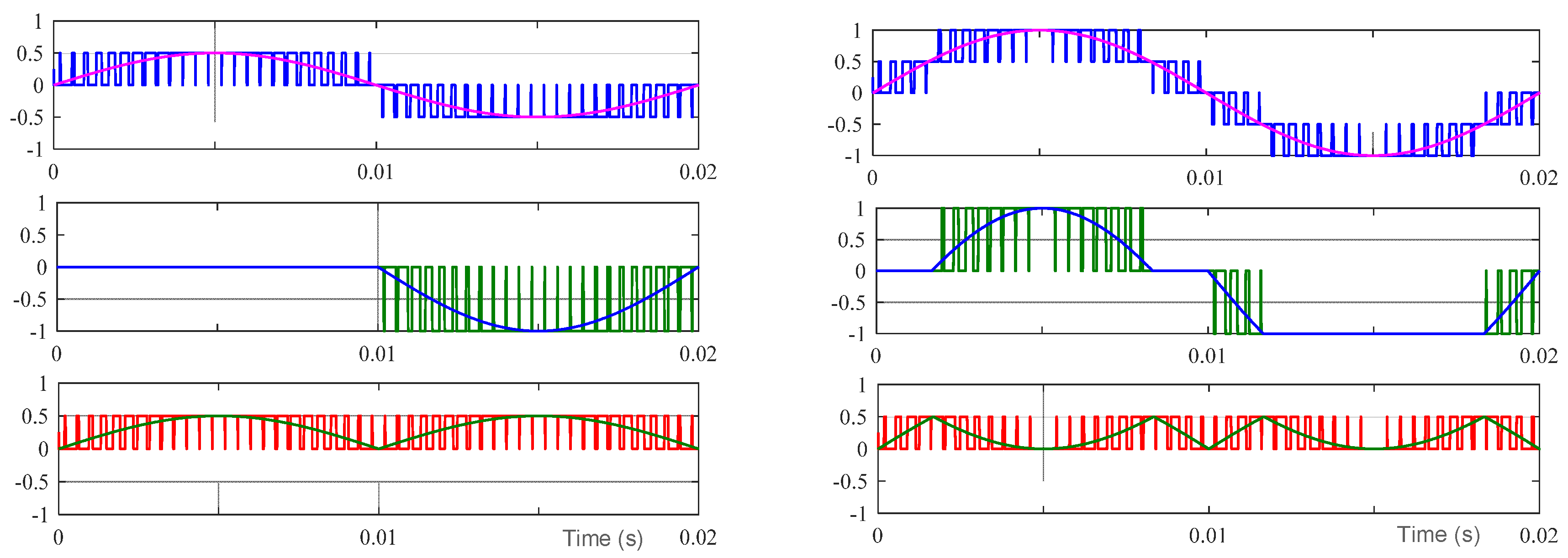
As an example of application of the above modulation principle, simulation results are given in case of m = 0.5 and m = 1. In particular, Figure 3 shows the modulating signals (1)–(4) and normalized instantaneous output voltages.

2.2. H-Bridge and LDN Output Voltage Harmonics

In order to determine the individual output voltage harmonics of both the H-bridge and LDN cells, the modulation symmetry of the LDN can be exploited. In particular, according to the waveform symmetry shown in Figure 3 (bottom traces), the harmonic spectrum contains only even harmonics with cosine terms (the LDN modulating signal is an even function).

The normalized LDN output voltage averaged over the switching period (Equation (2)), can be written in terms of harmonics as:

$$u_{ac}^L=U_0+{\displaystyle \sum _{k=2}^{\infty }{u}_k^L}=U_0+{\displaystyle \sum _{k=2}^{\infty }{U}_k}\cos (k\mathsf{\vartheta }).$$

(5)

where U₀ is the average component and |U_k| is the amplitude of the kth harmonic component, with k being an even number. The amplitude of these components are calculated analytically as:

$$U_0(m)=\{\begin{array}{cc}\frac{2}{\mathsf{\pi }}m\hfill & \hfill \mathrm{for}m\le 0.5\\ \frac{2}{\mathsf{\pi }}\left[m+\frac{\mathsf{\pi }}{2}-\arcsin (1/2m)-\sqrt{4m^2-1}\right]\hfill & \hfill \mathrm{for}m\ge 0.5\end{array},$$

(6)

$$U_k(m)=\{\begin{array}{cc}-\frac{4}{\mathsf{\pi }}\frac{m}{(k^2-1)}\hfill & \hfill \mathrm{for}m\le 0.5\\ \frac{4}{\mathsf{\pi }}\left[A_k(m)+B_k(m)\right]\hfill & \hfill \mathrm{for}m\ge 0.5\end{array}.$$

(7)

The expressions of the coefficients A_k (m) and B_k (m) in Equation (7) are given in the Appendix A.

Figure 4 shows the normalized amplitudes of low-order LDN output voltage harmonics over the whole modulation index range.

According to Equations (3) and (5), the normalized output voltage of the H-bridge is written as:

$$u_{ac}^H=-U_0+m\sin (\mathsf{\vartheta })-{\displaystyle \sum _{k=2}^{\infty }{U}_k}\cos (k\mathsf{\vartheta }).$$

(8)

The amplitudes of the harmonics in Equation (8) can be determined considering Equations (6) and (7). Comparing Equation (8) with Equation (5) it is evident that, compared to the LDN, the H-bridge has an additional first harmonic component U₁ = m. Figure 5 shows the normalized amplitudes of low-order H-bridge output voltage harmonics over the whole modulation index range.

3. PV Voltage and Current Harmonics

In the considered single-phase single-stage PV generation system (Figure 1), the PV field is directly connected to the input side of the H-bridge, so the PV field voltage corresponds to the H-bridge input voltage, whereas the PV current can be calculated on the basis of H-bridge input dc-link current and dc-link impedance, as shown in the following.

3.1. H-Bridge Input Current Harmonics

The instantaneous input dc-link current i^H of the H-bridge is composed by its averaged value over the switching period ${\overline{i}}^H$, and the instantaneous switching ripple $\Delta i^H$. Introducing also the average over the fundamental period I^H (dc component) and the alternating low-frequency harmonic component ${\tilde{i}}^H$,

$$i^H={\overline{i}}^H+\Delta i^H=I^H+{\tilde{i}}^H+\Delta i^H,$$

(9)

Considering the input–output H-bridge power balance for quantities averaged over the switching period, and normalizing by V, the input current is expressed as:

$${\overline{i}}^H={\overline{u}}_{ac}^H{\overline{i}}_{ac},$$

(10)

with ${\overline{i}}_{ac}$ being the output current averaged over the switching period. Supposing unity power factor and almost sinusoidal current, which is the basic requirement for most of grid-connected applications, it can be written as:

$${\overline{i}}_{ac}\cong i_{ac}=I_{ac}\sin \mathsf{\vartheta },$$

(11)

where $I_{ac}$ is the amplitude of the output current.

Replacing Equations (8) and (11) in Equation (10), the harmonic spectrum of the averaged H-bridge input current is obtained as (see Appendix A):

$${\overline{i}}^H=\frac{1}{2}\left[m+(2U_0-U_2)\sin \mathsf{\vartheta }-m\cos 2\mathsf{\vartheta }-{\displaystyle \sum _{n=3}^{\infty }(U_{n+1}-U_{n-1})\sin n\mathsf{\vartheta }}\right]I_{ac}.$$

(12)

where n is an odd number, n ≥ 3. Figure 6 shows the harmonic amplitudes appearing in Equation (12) as a function of the modulation index. It should be noted that the dc and second harmonic components have the same amplitude, proportional to the modulation index, as in the case of the H-bridge without LDN (Figure 1a). The first harmonic has a relevant amplitude, comparable to the amplitude of the second harmonic and aside from this in the third harmonic (that can be noticeable around m = 0.5 and m = 1), higher-order harmonics are quite negligible in the whole modulation range.

3.2. PV Voltage Harmonics

As for the current in Equation (9), the instantaneous H-bridge dc-link voltage v, corresponding to the PV voltage in the considered single-stage PV generation scheme, is composed of the averaged value over the switching period $\overline{v}$ and the instantaneous switching ripple Δv. Introducing the average over the fundamental period V (dc component) and the alternating low-frequency harmonic component $\tilde{v}$, it becomes:

$$v=\overline{v}+\Delta v=V+\tilde{v}+\Delta v\cong V+\tilde{v}.$$

(13)

The switching frequency component Δv is strongly smoothed by the dc-link capacitor, and it is usually negligible for switching frequencies starting from 5 to 10 kHz. It is assumed here that Δv ≅ 0.

The amplitude of the kth order harmonic component $V_k$ can be calculated as:

$$V_k^{}=Z_k{I}_k^H,$$

(14)

with $Z_k$ being the total dc-link impedance for the kth harmonic, given by the parallel between the reactance of the dc-link capacitor (C_H), and the equivalent resistance of the PV field (R_PV ≅ V_MPP/I_MPP in the vicinity of the MPP):

$$Z_k=\frac{R_{PV}}{\sqrt{{(R_{PV}k\mathsf{\omega }{C}_H)}^2+1}},$$

(15)

Considering realistic parameter values for PV fields and dc-link capacitors, the assumption R_PV >> 1/(kωC_H) is generally satisfied, and Equation (15) becomes:

$$Z_k=\frac{1}{k\mathsf{\omega }{C}_H}.$$

(16)

Using the previous assumption, Equation (14) can be written as:

$$V_k^{}=\frac{1}{k\mathsf{\omega }{C}_H}{I}_k^H$$

(17)

Introducing Equation (12) into Equation (17) and considering only the first and second dominating harmonic components, gives:

$$V_1^{}(m)=\frac{\left[U_2(m)-2U_0(m)\right]}{2\mathsf{\omega }{C}_H}{I}_{ac},$$

(18)

$$V_2^{}(m)=\frac{m}{4\mathsf{\omega }{C}_H}{I}_{ac}.$$

(19)

As an example, Figure 7 shows the amplitudes of the first and second PV voltage harmonics as a function of modulation index m, in the case that dc-link capacitor C_H = 1 mF, and there is unity sinusoidal output current.

3.3. PV Current Harmonics

As for the PV voltage v, the instantaneous PV current i can be written in terms of components, corresponding to Equation (13). Neglecting the switching frequency component, it becomes:

$$i=I+\tilde{i}$$

(20)

with I being the average over the fundamental period (dc component) and $\tilde{i}=\tilde{v}/R_{PV}$ the alternating low-frequency harmonic component. Note that, due to the dc-link capacitor, I = I^H.

Based on the amplitudes of PV voltage harmonics given by Equations (18) and (19), the amplitudes of the dominating first and second PV current harmonics can be written as:

$$I_1(m)=\frac{V_1^{}(m)}{R_{PV}}=\frac{U_2(m)-2U_0(m)}{2R_{PV}\mathsf{\omega }{C}_H}{I}_{ac},$$

(21)

$$I_2(m)=\frac{V_2^{}(m)}{R_{PV}}=\frac{m}{4R_{PV}\mathsf{\omega }{C}_H}{I}_{ac}.$$

(22)

As an example, Figure 8 shows the amplitudes of the first and second PV current harmonics as a function of modulation index m, in the case the dc-link capacitor C_H = 1 mF and there is unity sinusoidal output current, considering PV series equivalent resistance R_PV = 40 Ω, representing the scale factor with Figure 7.

According to Equations (18), (19), (21), and (22), it is clear that the amplitudes of the PV voltage and current harmonics are inversely proportional to the dc-link capacitor C_H since the dc-link capacitor reactance dominates the dc-link impedance. However, PV current harmonics also depend on the PV series-equivalent resistance R_PV, that is a function of the operating point on the PV field characteristic. Considering a PV plant of a few kW (single-phase), R_PV ranges between a few Ω near the open-circuit point, passing to around a few tens of Ω near the MPP and up to hundreds or even thousands of Ω toward the short-circuit point [26]. These considerations can be readily exploited to design the dc-link capacitor C_H in order to obtain PV voltage and current harmonics amplitude in the order of a few percent compared to the rated MPP values.

4. RCC-MPPT Algorithms in the Case of Single and Multiple PV Harmonics

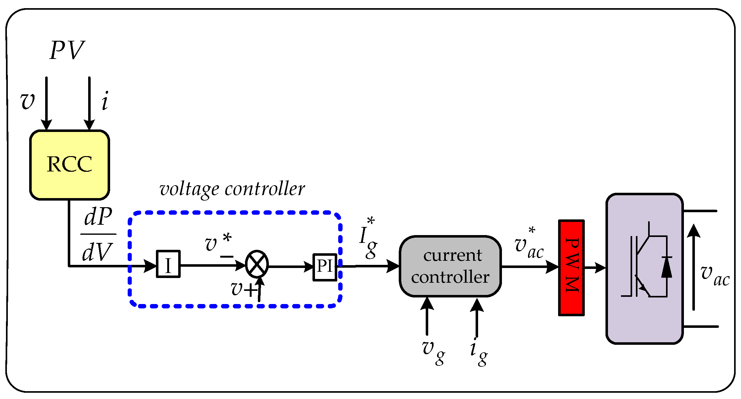
The block diagram of the whole PV control scheme considered in this paper is depicted in Figure 9. The RCC algorithm is used to estimate the voltage derivative of the power, dP/dV, driving the working point toward the MPP and determining the reference grid current amplitude I_g*. In particular, the reference dc-link voltage v* is simply obtained by integrating the estimated dP/dV, I_g* is determined by a PI voltage regulator, and the dq current controller has been implemented in order to inject a sinusoidal grid current with unity power factor.

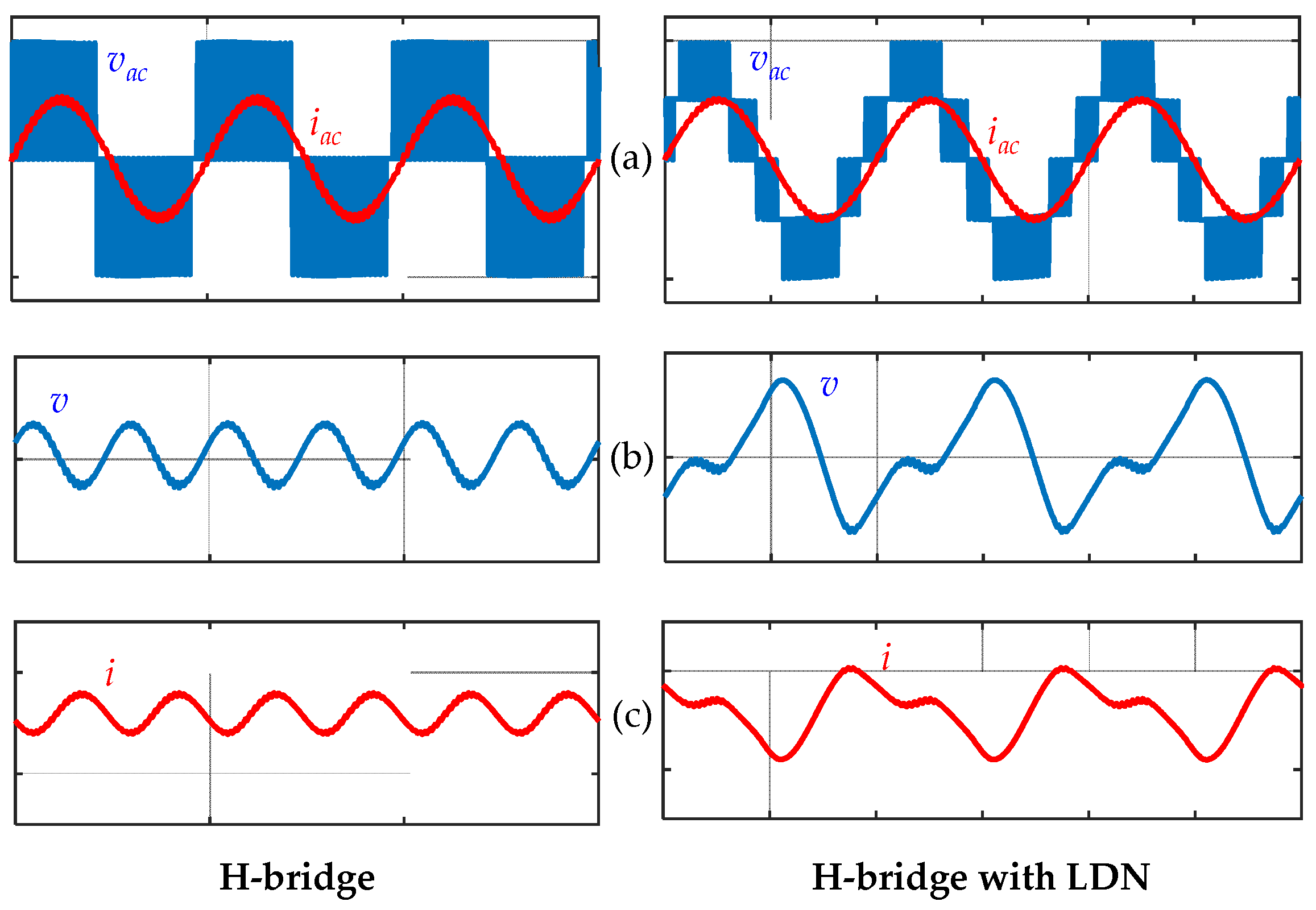
In order to provide for a comparative example of PV voltage and current oscillations in case of basic (H-bridge) and multilevel (H-bridge with LDN) inverter configurations, Figure 10 shows the results of a numerical simulation considering the two conversion schemes in the same working conditions. It is clearly visible that PV voltage and current contain only the second harmonic (100 Hz) in the case of H-bridge without LDN (left column). Increasing the number of the output voltage level from 3 to 5 with the considered LDN configuration, a relevant first harmonic (50 Hz) clearly appears in addition to the second harmonic in both PV voltage and current.

4.1. Basic RCC-MPPT Algorithm in Case of Single PV Harmonic

In case of single-phase single-stage PV systems, with the inverter being directly connected to the PV field, inherent second-order harmonics of instantaneous power appear in the PV current and PV voltage. As is known, the ripple correlation control algorithm uses these oscillations for providing information about the operating point of the PV field. For the considered working point Q, the voltage derivative of the PV power dP/dV is written as:

$${\frac{dP}{dV}|}_Q=I+{\frac{dI}{dV}|}_{Q}V$$

(23)

where dI/dV defines the relation between PV current and PV voltage harmonics as:

$$\tilde{i}={\frac{dI}{dV}|}_Q\tilde{v}$$

(24)

Generally speaking, the most popular RCC-MPPT implementation consists in multiplying the voltage harmonic by the current harmonic, and integrating over the harmonic period, i.e., half of fundamental (grid) period T/2, as:

$${\frac{dI}{dV}|}_Q=\frac{{\displaystyle \underset{t-T/2}{\overset{t}{\int }}\tilde{i}\tilde{v}dt}}{{\displaystyle \underset{t-T/2}{\overset{t}{\int }}{\tilde{v}}^{2}dt}}=-\frac{I_2{V}_2}{V_2^2}=-\frac{I_2}{V_2}$$

(25)

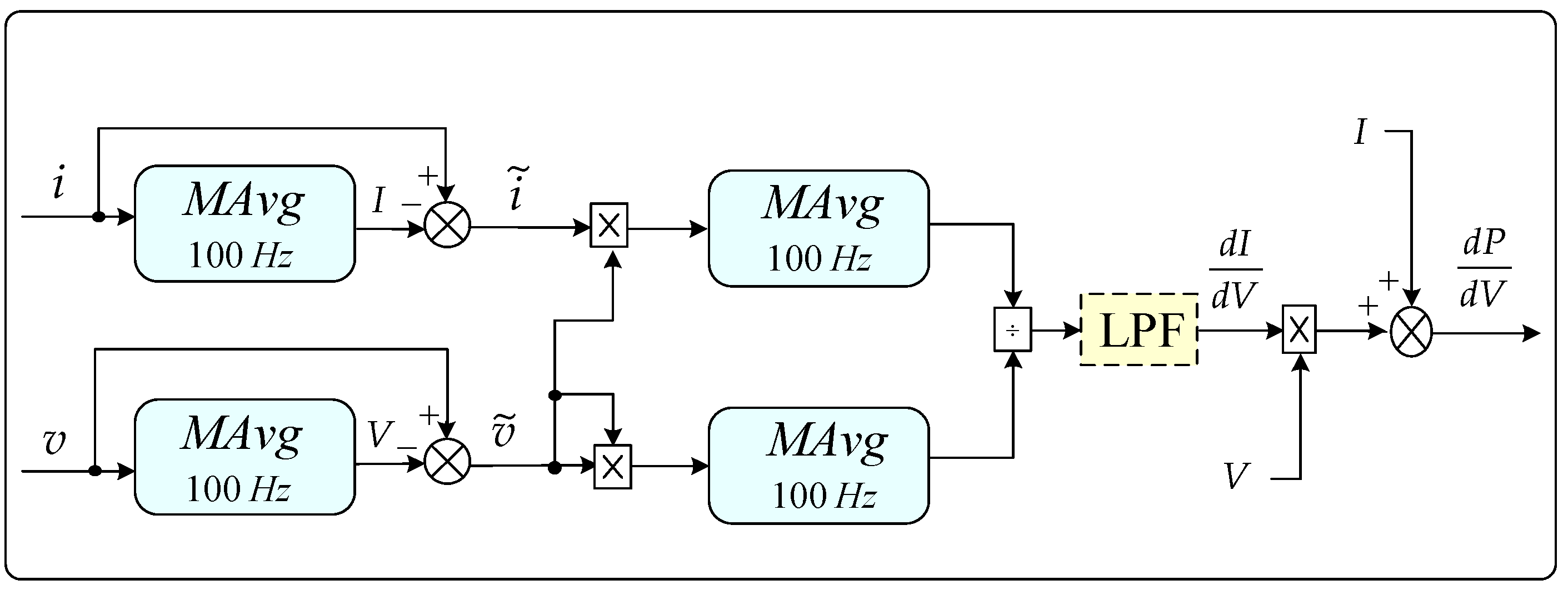
Assuming the fundamental output period T (frequency 50 Hz), the concept of moving average (MAvg) is introducing over T/2 (100 Hz) in Equation (25), and Equation (23) can be rewritten in terms of block diagram representing the estimation of dP/dV, with $\tilde{v}$ and $\tilde{i}$ being calculated by Equation (13) and Equation (20), respectively, as shown in Figure 11.

4.2. The Proposed RCC-MPPT Algorithm in the Case of Multiple PV Harmonics

In case of multiple PV voltage and current harmonics (multilevel topology), the estimation of dI/dV (and then dP/dV) should be carried out by considering a specific harmonic (kth order), preferably the one with highest amplitude to increase the resolution. In this case, Equation (24) can be rewritten as:

$${\tilde{i}}_k={\frac{dI}{dV}|}_Q{\tilde{v}}_k$$

(26)

By following the same approach as in previous sub-section, Equation (25) can be summarized for each considered harmonic as:

$${\frac{dI}{dV}|}_Q^k=\frac{{\displaystyle \underset{t-T}{\overset{t}{\int }}{\tilde{i}}_k{\tilde{v}}_{k}dt}}{{\displaystyle \underset{t-T}{\overset{t}{\int }}{\tilde{v}}_k^{2}dt}}=-\frac{I_k{V}_k}{V_k^2}=-\frac{I_k}{V_k}.$$

(27)

Note that integrals in Equation (27) are now calculated over the fundamental period T (corresponding to the grid frequency), as defined by the Fourier series, to calculate the kth harmonic. The implementation of Equation (27) is shown in the block diagram of Figure 12, estimating the dP/dV considering only the kth harmonic component.

An alternative approach consists in extending the period of the moving average in the basic RCC scheme of Figure 11 from half of the period (T/2) to the whole fundamental period T (from 100 Hz to 50 Hz), according to:

$${\frac{dI}{dV}|}_Q=\frac{{\displaystyle \underset{t-T\text{}}{\overset{t}{\int }}\tilde{i}\tilde{v}dt}}{{\displaystyle \underset{t-T\text{}}{\overset{t}{\int }}{\tilde{v}}^{2}dt}}$$

(28)

The corresponding block diagram to estimate dP/dV is presented in Figure 13.

The relationship between the single harmonic method given by Equation (27) and the extended moving average method (Equation (28)) can be carried out by considering all the harmonics of the alternating PV voltage and current components:

$$\tilde{v}={\displaystyle {\sum }_k{\tilde{v}}_k^{}},\tilde{i}={\displaystyle {\sum }_k{\tilde{i}}_k^{}}$$

(29)

In fact, considering Parseval’s theorem and introducing Equation (29) into Equation (28), the estimation of dI/dV can be written as:

$${\frac{dI}{dV}|}_Q=\frac{{\displaystyle \underset{t-T}{\overset{t}{\int }}{\displaystyle {\sum }_k{\tilde{i}}_k}{\displaystyle {\sum }_k{\tilde{v}}_k}dt}}{{\displaystyle \underset{t-T}{\overset{t}{\int }}{({\displaystyle {\sum }_k{\tilde{v}}_k})}^{2}dt}}=-\frac{{\displaystyle {\sum }_k{I}_k{V}_k}}{{\displaystyle {\sum }_k{V}_k^2}}$$

(30)

Equation (30) can be reorganized multiplying and dividing by V_k, as follows:

$${\frac{dI}{dV}|}_Q=-\frac{{\displaystyle {\sum }_k(V_k^2\frac{I_k}{V_k})}}{{\displaystyle {\sum }_k{V}_k^2}}=\frac{{\displaystyle {\sum }_k({w_k\frac{dI}{dV}|}_Q^k)}}{{\displaystyle {\sum }_k{w}_k}}$$

(31)

Equation (31) states that the estimation of dI/dV made by the modified moving average method (28) (i.e., MAvg over the fundamental period T) is equivalent to the weighted average of the estimation of dI/dV obtained by the individual harmonics (Equation (27)), using as weight (w_k) the square of the kth voltage harmonic amplitude:

$$w_k=V_k^2.$$

(32)

In order to preliminarily prove the effectiveness of modified RCC compared to the basic RCC for the estimation of dP/dV, a simulation example is given in Figure 14. In particular, considering a simple linear I-V curve corresponding to a parabolic P-V curve, the dP/dV is calculated by the basic RCC scheme of Figure 11 (MAvg over T/2, 100 Hz, top), and the modified RCC scheme of Figure 13 (MAvg over T, 50 Hz, bottom), in the case of H-bridge with LDN (i.e., Figure 1b, and Figure 10, right column). Reference is made to the two steady-state operating points symmetrically placed on the left- and on the right-side of the MPP, corresponding to dP/dV ≅ ±0.25 A, as depicted in Figure 14. It is evident that applying the MAvg at 100 Hz results in an oscillating estimation of dP/dV, whereas the estimation is precise and stable applying the MAvg at 50 Hz, as a consequence of Equation (31).

5. Implementation and Experimental Results

In order to verify the effectiveness of the multilevel PV inverter with the proposed RCC-MPPT algorithms in both steady-state and transient conditions, a grid-connected PV generation system with H-bridge and LDN has been implemented, according to the circuit scheme of Figure 15.

The picture of the corresponding experimental setup is shown in Figure 16. It consists of two power boards (H-bridge and LDN) based on Mitsubishi insulated-gate bipolar transistor (IGBT) smart modules, IPM PS22A76 (1200 V, 25 A, Mitsubishi Electric Corporation, Tokyo, Japan), Yokogawa DLM 2024 oscilloscope (Yokogawa Electric Corporation, Tokyo, Japan) with the PICO TA057 differential voltage probe (25 MHz, ±1400 V, ±2%, Pico Technology, Tyler, TX, USA), and LEM PR30 current probe (dc to 20 kHz, ±20 A, ±1%, LEM Europe GmbH, Fribourg, Switzerland). Additionally, two current transducers of the LA 55-P model (LEM^® Company, Geneva, Switzerland) were used to measure PV and grid currents, while PV and grid voltages were measured using two voltage transducers of the LV 25-P model (LEM^® Company, Geneva, Switzerland). The switching frequency of the multilevel grid-connected inverter is set to 2.5 kHz. For digital implementation of current and voltage controllers, as well as the phase-locked loop (PLL) and the RCC-MPPT algorithms, a digital signal processor (DSP TMS320F28377D) was used to generate the PWM signals for the H-bridge and the LDN boards of the multilevel LDN inverter. An optical interface board links DSP with power boards. Results are shown by oscilloscope screenshots, elaborating and emphasizing the signals of interest. The main parameters of the experimental setup are given in

Table 1. Parameters of the conversion system.

Label	Description	Parameters
CH	dc-link H-bridge capacitance	2.2 mF
CL	dc-link LDN capacitance	3.3 mF
Cf	ac filter capacitance	25 μF
Rf, Lf	ac filter resistance and inductance	1.1 Ω, 8.8 mH
fsw	switching frequency	2.5 kHz
Vg	grid voltage (RMS) (1:10 transformer)	22/220 V
f	grid (fundamental) frequency	50 Hz

.

The dc source has been implemented by a resistive voltage supply with variable series resistance for preliminary steady-state and transient tests, according to the scheme of Figure 15. The corresponding parameters are given in

Table 2. Resistive dc source parameters.

Label	Description	Parameters
VS	dc voltage supply	100 V
R1, R2	dc source resistance (RS)	40 Ω, 20 Ω

.

For realistic tests, a reduced-scale array consisting of two series-connected PV modules has been adopted, introducing different irradiance conditions by covering/uncovering with a white sheet, well representing sunny and cloudy conditions (the sun irradiance on the PV module surface ranges between approximately 100% and 40%), as shown in the right side of Figure 16. PV modules, placed on the roof of the building, supply the conversion system in the Lab at the ground floor using a connection cable (length of approximately 40 m). The main parameters of the PV source are given in

Table 3. PV source parameters—Standard test conditions (STC).

Label	Description	Parameters
VOC	open circuit voltage	43.4 V
ISC	short circuit current	4.8 A
VMPP	maximum photovoltaic voltage	34 V
IMPP	maximum photovoltaic current	4.4 A
NS	number of series-connected PV modules	2
Rc, Lc	resistance and inductance of PV cable	0.5 Ω, 40 μH

, whereas the corresponding I-V and P-V characteristics, obtained from the Lab by the charging transient of a capacitor (1 mF), are given in Figure 17.

The first test is carried out in order to verify the input/output steady-state waveforms of the considered multilevel inverter, in the grid-connected configuration shown in Figure 15 with resistive dc supply (linear-equivalent PV source). In particular, Figure 18a shows grid voltage and current (top half screen) and PV voltage and current (bottom half screen), whereas Figure 18b shows the time zoom of inverter voltage and current (top half screen) and PV voltage and current (bottom half screen). As expected, the inverter voltage has a proper multilevel waveform over five levels, and inverter (grid) current is almost sinusoidal despite the switching frequency being only 2.5 kHz, with unity power factor. PV voltage and PV current have oscillations, including both first and second harmonic components (50 and 100 Hz, respectively), in phase opposition.

The following tests are carried out in order to verify the dynamic performance of the different RCC-MPPT algorithms in the case of irradiance transients. In particular, two sets of experimental tests have been considered. In the first tests presented in Figure 19 and Figure 20 the linear-equivalent PV source has been selected in order to simulate extremely fast irradiance transients by switching on/off the series resistances, performing dynamic comparative tests for all the four types of RCC-MPPT algorithms. The last tests presented in Figure 21 are performed considering the real PV source, introducing irradiance transients by shadowing/unshadowing the PV modules by a white sheet, well representing the effects of real clouds (Figure 16 and Figure 17).

Figure 19 shows grid voltage and current (top half screen) as well as PV voltage and current (bottom half screen) in the case of transients obtained by switching on/off the series resistances (Figure 15, Table 2), representing a step irradiance transient. Diagrams in Figure 19a are obtained by the basic RCC scheme with low-pass filters based on MAvg over T/2 (100 Hz, corresponding to Figure 11), whereas diagrams in Figure 19b are obtained by the modified RCC scheme with low-pass filters based on MAvg over T (50 Hz, corresponding to Figure 13).

In both cases, as expected, the steady-state MPP voltage is equal to the half of the dc source voltage (V_S = 100V, V_MPP = 50V). In this case, the (equivalent) irradiance step is seen as a perturbation by the PV voltage controller. Correspondingly, the PV current shows a fast step transient.

Despite the basic RCC scheme giving acceptable results, it leads to larger overshoots and higher settling times comparing to the modified RCC.

Figure 20 shows the same quantities with the same kind of transients as in Figure 19, but referred to the modified RCC schemes employing only a specific harmonic component (reference is made to Figure 12). In particular, diagrams in Figure 20a are obtained by the modified RCC scheme based on the 2nd harmonic component (100 Hz), whereas diagrams in Figure 20b are obtained by the modified RCC scheme based on the first harmonic component (50 Hz). Both these modified RCC-MPPT schemes give similar results, being similar the amplitude of voltage and current harmonics (Figure 7 and Figure 8), with smoothed overshoots and short settling times for the PV variables.

In particular, the modified RCC scheme employing the first harmonic component (50 Hz) seems to be more effective, also offering the advantage of using the highest harmonic amplitude in the typical modulation index range for grid-connected PV generation schemes (i.e., m between 0.7 and 0.8). For these reasons, only this last modified RCC-MPPT scheme is considered in the last tests presented in Figure 21, considering a real PV source (two PV modules), in real environmental operating conditions, and with realistic irradiance transients. Increasing and decreasing sun irradiance transients obtained by shadowing and unshadowing the PV modules by a white sheet have been considered, corresponding to the P-V and I-V characteristics of Figure 17 (500 W/m² and 200 W/m²).

In particular, Figure 21 shows grid voltage and current (top half of the screen), together with PV voltage and the estimation of dP/dV (bottom half of the screen). As expected, the estimation of dP/dV fails during the initial part of the transient, but without introducing particular drawbacks in PV and grid variables. In fact, both for increasing and decreasing irradiance transients, grid current amplitude has a smoothed and fast profile, without significant overshoots.

6. Efficiency Analysis in Comparison to the Basic H-Bridge Configuration

As a final remark, the proposed multilevel conversion scheme, in Figure 1b, is compared with the basic H-bridge conversion scheme, in Figure 1a, from the point of view of the overall efficiency. In particular, a comparative estimation of power losses is carried out introducing some simplifying assumptions.

Generally speaking, the multilevel converter itself has one additional leg (with two additional power switches), i.e., three legs instead of two, with a consequent increase in conduction and switching losses being the main disadvantage of multilevel configurations. On the other hand, the reduced harmonic distortion in multilevel output voltage (inter-level voltage excursion is half, passing from 3 to 5 levels) makes it possible to reduce the inductance (L_f) of the ac-link inductor to obtain the same grid current distortion, reducing inductor losses. This is one of the known advantages of multilevel configurations.

With reference to the multilevel inverter losses, for the LDN leg in series with the two H-bridge legs, they share the same current, so each leg has the same conduction losses. The steady-state voltage the half in the LDN leg, as discussed in Section 2, the switching losses in the LDN leg are the half compared to the switching losses in the individual H-bridge legs. Supposing conduction and switching losses equally shared, as in most of the switching converter design, the additional LDN leg introduces 50% more of the conduction losses, and 25% more of the switching losses. So, comparing to the basic H-bridge inverter, the multilevel inverter has almost 37.5% of additional losses.

With reference to the ac-link inductor, in case of multilevel inverter, it can be designed for the half of the inductance (L_f/2) compared to the basic H-bridge scheme (L_f), since the voltage harmonic distortion is almost half, leading to almost the same current harmonic distortion. Supposing the use of the same amount of copper for the reactor winding, and neglecting the core losses (if any), the copper losses are reduced to 50%, with the winding resistance reduced to half (turns are √2 times less and the wire cross area can be √2 times more to have the same copper weight), and the ac-link reactor current the same.

All in all, a real benefit in terms of efficiency can be experienced in the case of the multilevel inverter (H-bridge + LDN) compared to basic inverter (only H-bridge) especially in case of an overall conversion system design with lower inverter losses (that are increased 37.5%) compared to ac-link inductor losses (that are decreased by 50%).

7. Conclusions

In this paper, a single-phase single-stage PV generation system with multilevel output voltage waveforms and an improved RCC-MPPT algorithm has been proposed and examined in detail. The multilevel inverter is implemented by an LDN cell, as a kind of retrofit to the basic H-bridge cell, increasing the output voltage levels from three to five. In addition to the second harmonic resulting from the basic H-bridge configuration, a multilevel configuration introduces additional voltage and current harmonics on the input (PV) side. In particular, a relevant first-order harmonic is noticeable, the third harmonic is slightly appreciable, whereas higher-order harmonics are completely negligible. Both PV voltage and current harmonic amplitudes are analytically calculated in the whole modulation range, offering the possibility of a precise and effective design of the dc-link capacitor to satisfy the ripple requirements.

Due to the additional harmonics, the basic RCC-MPPT scheme becomes inadequate, leading to a misestimation of dP/dV. A modified RCC scheme extracting the amplitude of a specific harmonic from PV voltage and current waveforms has been proposed in order to overcome this drawback. Reference has been made to the harmonic with highest amplitude in order to maximize the resolution, leading to a correct and precise estimation of dP/dV. It has been verified that a correct estimation of dP/dV can be simply obtained by doubling the time window of low-pass filters in the RCC scheme (i.e., moving average, from T/2 to T). It has been proven that the resulting dP/dV is a weighted average of all the dP/dV estimations performed by the individual PV voltage and current harmonics, the weight being the individual voltage harmonic amplitude itself.

Numerical and experimental tests have been carried out to prove the effectiveness of the whole PV generation scheme, including multilevel waveforms and improved RCC-MPPT algorithms. Both the linear-equivalent PV source and real PV sources have been implemented in the experimental setup, considering both steady-state and fast sun irradiance transient conditions in order to verify the dynamic performance of the different RCC-MPPT methods.

References

- Kjaer, S.B.; Pedersen, J.K.; Blaabjerg, F. A Review of Single-Phase Grid-Connected Inverters for Photovoltaic Modules. IEEE Trans. Ind. Appl. 2005, 41, 1292–1306. [Google Scholar] [CrossRef]
- Tobón, A.; Peláez-Restrepo, J.; Villegas-Ceballos, J.; Serna-Garcés, S.; Herrera, J.; Ibeas, A. Maximum Power Point Tracking of Photovoltaic Panels by Using Improved Pattern Search Methods. Energies 2017, 10, 1316. [Google Scholar] [CrossRef]
- Na, W.; Chen, P.; Kim, J. An Improvement of a Fuzzy Logic-Controlled Maximum Power Point Tracking Algorithm for Photovoltic Applications. Appl. Sci. 2017, 7, 326. [Google Scholar] [CrossRef]
- Ozturk, S.; Cadirci, I. A Generalized and Flexible Control Scheme for Photovoltaic Grid-Tie Microinverters. IEEE Trans. Ind. Appl. 2017. [Google Scholar] [CrossRef]
- Bazzi, A.M.; Krein, P.T. Ripple Correlation Control: An Extremum Seeking Control Perspective for Real-Time Optimization. IEEE Trans. Power Electron. 2014, 29, 988–995. [Google Scholar] [CrossRef]
- Khanna, R.; Zhang, Q.; Stanchina, W.E.; Reed, G.F.; Mao, Z.H. Maximum Power Point Tracking Using Model Reference Adaptive Control. IEEE Trans. Power Electron. 2014, 29, 1490–1499. [Google Scholar] [CrossRef]
- De Brito, M.A.G.; Galotto, L.; Sampaio, L.P.; De Azevedo Melo, G.; Canesin, C.A. Evaluation of the Main MPPT Techniques for Photovoltaic Applications. IEEE Trans. Ind. Electron. 2013, 60, 1156–1167. [Google Scholar] [CrossRef]
- Elsaharty, M.A.; Ashour, H.A.; Rakhshani, E.; Pouresmaeil, E.; Catalão, J.P.S. A Novel DC-Bus Sensor-Less MPPT Technique for Single-Stage PV Grid-Connected Inverters. Energies 2016, 9, 248. [Google Scholar] [CrossRef]
- Casadei, D.; Grandi, G.; Rossi, C. Single-Phase Single-Stage Photovoltaic Generation System Based on a Ripple Correlation Control Maximum Power Point Tracking. IEEE Trans. Energy Convers. 2006, 21, 562–568. [Google Scholar] [CrossRef]
- Hammami, M.; Grandi, G.; Rudan, M. An Improved MPPT Algorithm Based on Hybrid RCC Scheme for Single-Phase PV Systems. In Proceedings of the 42nd Annual Conference of the IEEE Industrial Electronics Society (IECON), Florence, Italy, 23–26 October 2016; pp. 3024–3029. [Google Scholar]
- Esram, T.; Kimball, J.W.; Krein, P.T.; Chapman, P.L.; Midya, P. Dynamic Maximum Power Point Tracking of Photovoltaic Arrays Using Ripple Correlation Control. IEEE Trans. Power Electron. 2006, 21, 1282–1290. [Google Scholar] [CrossRef]
- Paz, F.; Ordonez, M. High-Performance Solar MPPT Using Switching Ripple Identification Based on a Lock-in Amplifier. IEEE Trans. Ind. Electron. 2016, 63, 3595–3604. [Google Scholar] [CrossRef]
- Hammami, M.; Grandi, G.; Rudan, M. RCC-MPPT Algorithms for Single-Phase PV Systems in Case of Multiple Dc Harmonics. In Proceedings of the 6th International Conference on Clean Electrical Power: Renewable Energy Resources Impact ICCEP, Santa Margherita Ligure, Liguria, Italy, 27–29 June 2017; pp. 678–683. [Google Scholar]
- Rahim, N.A.; Selvaraj, J. Multistring Five-Level Inverter with Novel PWM Control Scheme for PV Application. IEEE Trans. Ind. Electron. 2010, 57, 2111–2123. [Google Scholar] [CrossRef]
- Yuan, X.; Stemmler, H.; Barbi, I. Self-Balancing of the Clamping-Capacitor-Voltages in the Multilevel Capacitor-Clamping-Inverter under Sub-Harmonic PWM Modulation. IEEE Trans. Power Electron. 2001, 16, 256–263. [Google Scholar]
- Babaei, E.; Laali, S.; Bayat, Z. A Single-Phase Cascaded Multilevel Inverter Based on a New Basic Unit with Reduced Number of Power Switches. IEEE Trans. Ind. Electron. 2015, 62, 922–929. [Google Scholar] [CrossRef]
- Buticchi, G.; Barater, D.; Lorenzani, E.; Concari, C.; Franceschini, G. A Nine-Level Grid-Connected Converter Topology for Single-Phase Transformerless PV Systems. IEEE Trans. Ind. Electron. 2014, 61, 3951–3960. [Google Scholar] [CrossRef]
- Debnath, S.; Qin, J.; Bahrani, B.; Saeedifard, M.; Barbosa, P. Operation, Control, and Applications of the Modular Multilevel Converter: A Review. IEEE Trans. Power Electron. 2015, 30, 37–53. [Google Scholar] [CrossRef]
- Orfanoudakis, G.I.; Sharkh, S.M.; Yuratich, M. Analysis of Dc-Link Capacitor Current in Three-Level Neutral Point Clamped and Cascaded H-Bridge Inverters. IET Power Electron. 2013, 6, 1376–1389. [Google Scholar] [CrossRef]
- Nabae, A.; Takahashi, I.; Akagi, H. A New Neutral-Point-Clamped PWM Inverter. IEEE Trans. Ind. Appl. 1981, IA-17, 518–523. [Google Scholar] [CrossRef]
- Daher, S.; Schmid, J.; Antunes, F.L.M. Multilevel Inverter Topologies for Stand-Alone PV Systems. IEEE Trans. Ind. Electron. 2008, 55, 2703–2712. [Google Scholar] [CrossRef]
- Chattopadhyay, S.K.; Chakraborty, C. A New Multilevel Inverter Topology with Self-Balancing Level Doubling Network. IEEE Trans. Ind. Electron. 2014, 61, 4622–4631. [Google Scholar] [CrossRef]
- Chattopadhyay, S.K.; Chakraborty, C. A New Asymmetric Multilevel Inverter Topology Suitable for Solar PV Applications with Varying Irradiance. IEEE Trans. Sustain. Energy 2017, 8, 1496–1506. [Google Scholar] [CrossRef]
- Vujacic, M.; Hammami, M.; Srndovic, M.; Grandi, G. Theoretical and Experimental Investigation of Switching Ripple in the DC-Link Voltage of Single-Phase H-Bridge PWM Inverters. Energies 2017, 10, 1189. [Google Scholar] [CrossRef]
- Vujacic, M.; Srndovic, M.; Hammami, M.; Grandi, G. Evaluation of DC Voltage Ripple in Single-Phase H-Bridge PWM Inverters. In Proceedings of the 42nd Annual Conference of the IEEE Industrial Electronics Society (IECON), Florence, Italy, 23–26 October 2016; pp. 3235–3240. [Google Scholar]
- Suntio, T.; Messo, T.; Aapro, A.; Kivimäki, J.; Kuperman, A. Review of PV Generator as an Input Source for Power Electronic Converters. Energies 2017, 10, 1076. [Google Scholar] [CrossRef]
Figure 1.
Single-phase single-stage photovoltaic (PV) generation system: (a) basic H-bridge configuration; (b) H-bridge plus level doubling network (LDN) multilevel configuration.
Figure 2.
Modulation principle for multilevel pulse-width modulation: carriers and modulating signals for H-bridge (top) and LDN (bottom) in the case of m = 0.5 (left) and m = 1 (right).
Figure 3.
Simulation results (fsw = 2.5 kHz): modulating signals and instantaneous output voltages normalized by V: total (top), H-bridge (middle), and LDN (bottom) in the case of m = 0.5 (left) and m = 1 (right).
Figure 4.
Normalized amplitudes of low-order LDN output voltage harmonics as a function of the modulation index.
Figure 5.
Normalized amplitudes of the low-order H-bridge output voltage harmonics as a function of the modulation index.
Figure 6.
Amplitudes of low-order H-bridge input current harmonics for sinusoidal unity output current as a function of the modulation index.
Figure 7.
Amplitude of dominating low-frequency PV voltage harmonics as a function of the modulation index in case CH = 1 mH and Iac = 1 A.
Figure 8.
Amplitude of dominating low-frequency PV current harmonics as a function of the modulation index in the case CH = 1 mH, Iac = 1 A, and RPV = 40 Ω.
Figure 9.
Block diagram of the whole PV control scheme. RCC: ripple correlation control.
Figure 10.
Simulation examples of: (a) grid current and inverter output voltage; (b) PV voltage; and (c) PV current, in case of H-bridge without LDN (left column), and in case of H-bridge with LDN (right column).
Figure 11.
Block diagram of the basic RCC algorithm to estimate dP/dV in the case of existence of a single harmonic component (second harmonic) using MAvg over T/2 (100 Hz).
Figure 12.
Block diagram of proposed RCC estimating dP/dV by a specific harmonic (Fourier series, FS).
Figure 13.
Block diagram of the modified RCC algorithm to estimate dP/dV extending MAvg over T (50 Hz).
Figure 14.
Simulation results: steady-state estimation of dP/dV by RCC with moving average over different periods and working points on the left (V1* = 45 V) and on the right (V2* = 55 V) of the MPP (VMPP = 50 V). Top traces: MAvg over T/2 (100 Hz, basic RCC), and bottom traces: MAvg over T (50 Hz, modified RCC).
Figure 15.
Circuit scheme of the experimental setup including the whole PV generation system.
Figure 16.
Picture view of the experimental setup in the lab (left side) and arrangement of the PV array (two modules) on the roof, free and shadowed by a white sheet (≅500 W/m2 and 200 W/m2, right side).
Figure 17.
P-V and I-V characteristics of the PV array including the cable (Table 2) with an irradiance of 500 W/m2 (top) and 200 W/m2 (white sheet, bottom) and Tcell ≅ 35 °C (reference is made to Figure 16).
Figure 18.
Input/output steady-state waveforms of the converter with VS = 100 V, RS = 60 Ω, V = VMPP = 50 V: (a) grid voltage and current (top traces), PV voltage and current (bottom traces); (b) time zoom: inverter voltage and current (top traces), PV voltage and current (bottom traces).
Figure 19.
Experimental results of RCC-MPPT algorithms in case of step transients of RS: (a) low-pass filters by MAvg over T/2 (100 Hz) and (b) low-pass filters MAvg over T (50 Hz). Top traces: grid voltage and current. Bottom traces: PV voltage and current.
Figure 20.
Experimental results of modified RCC-MPPT algorithms in the case of step transients of RS: (a) using only the second harmonic component (100 Hz); and (b) using only the first harmonic component (50 Hz). Top traces: grid voltage and current. Bottom traces: PV voltage and current.
Figure 21.
Decrease and increase sun irradiance transients (500 W/m2–200 W/m2) using only the 50-Hz harmonic component (Fourier).