Improving an Integer Linear Programming Model of an Ecovat Buffer by Adding Long-Term Planning

Abstract

The Ecovat is a seasonal thermal storage solution consisting of a large underground water tank divided into a number of virtual segments that can be individually charged and discharged. The goal of the Ecovat is to supply heat demand to a neighborhood throughout the entire year. In this work, we extend an integer linear programming model to describe the charging and discharging of such an Ecovat buffer by adding a long-term (yearly) planning step to the model. We compare the results from the model using this extension to previously obtained results and show significant improvements when looking at the combination of costs and the energy content of the buffer at the end of the optimization. Furthermore, we show that the model is very robust against prediction errors. For this, we compare two different cases: one case in which we assume perfect predictions are available and one case in which we assume no predictions are available. The largest observed difference in costs between these two cases is less than 2%.

1. Introduction

In an effort to reduce green house gas emissions, as well as the dependency on the finite supply of fossil fuels, we see an increasing trend towards the use of renewable alternatives. However, one of the disadvantages of such renewables is that their generation peaks rarely coincide with peaks in demand, both on a daily basis and on a seasonal scale. One way to overcome this problem is the introduction of thermal storage (see, e.g., [1,2]) into the system. Much research has been done on such thermal storage (for an overview of thermal storage technologies, see, e.g., [3]), as well as on seasonal thermal storage in particular (e.g., [4]). The Ecovat buffer is such a seasonal thermal storage technology and falls into the category of sensible storage systems. Such sensible thermal storage systems store energy by increasing the temperature of their storage medium. The most popular choice of storage medium is water due to its availability, low cost and high specific heat. Another popular choice is to use rocks as the storage medium. An advantage of rocks compared to water is that they can be heated to higher temperatures, while a disadvantage is a much lower energy density. The storage medium used in the Ecovat system is water. Sensible storage systems using water as the storage medium include water tanks [5,6], solar ponds [7] and aquifers [8]. For a system using rocks as the storage medium, see for example [9]. Other thermal storage technologies include latent thermal storage and chemical thermal storage. In latent thermal storage energy is stored by means of a phase change in the storage medium (phase change materials). Compared to sensible storage, latent storage can achieve much larger energy densities, while operating on smaller temperature ranges due to the nearly constant temperature at which such phase changes occur. A disadvantage is the generally higher investment costs involved with latent storage. Reviews on thermal storage involving phase change materials are presented in for example [10,11]. Chemical thermal storage stores energy by means of reversible chemical reaction or sorption processes. Chemical storage has an even higher energy density than latent storage. However, the disadvantage is that it is also more expensive currently. For a review on chemical storage, see for example [12].

For the supply of heat demand to houses, a number of options is currently considered in the literature, ranging from residential water heaters, potentially in combination with a small storage tank (e.g., [13,14]), to district heating networks that supply heat to an entire neighborhood. District heating networks might cover a significant portion of the future heating demand in large parts of Europe as discussed in [15]. The heat in such a district heating network can be supplied in a number of ways, for example by large-scale heat pumps (reviewed in [16]) or by combined heat and power units to supply both heat and electricity to a neighborhood (e.g., [17]). In the future, the Ecovat system could also be combined with a district heating network to supply the heat demand of a neighborhood, by storing heat at times it is available, for example from renewable energy sources, until it is required by the district heating network to supply the heat demand.

The Ecovat [18] system consists of a large underground water tank, the Ecovat buffer, consisting of a number of (virtual) horizontal segments. These segments can be individually charged and discharged using heat exchangers integrated into the buffer walls. However, as the water in these segments is not physically separated, it is important to keep the thermal stratification within the buffer intact while charging and discharging the buffer, since this leads to a higher performance [19,20]. An overview of thermal stratification in water tanks is given by [21]. The Ecovat buffer is accompanied by a number of heat pumps, photovoltaic thermal panels (PVT) and a resistance heater, which can be used as energy sources.

In previous work [22], we developed an integer linear programming (ILP) model to optimize the charging and discharging of an Ecovat buffer. In that model, the aim is to optimize over a long time horizon (a year), which is necessary since the Ecovat buffer is a seasonal thermal storage system. However, it is also important to consider short time intervals since the electricity market operates on short time scales (15 min). This combination of a long time horizon and short time intervals leads to an ILP model with a large number of variables. A consequence of this is that it is not possible to optimize over the entire time horizon at once. Because of this, in [22], a rolling horizon approach was employed, which in every step only optimized over the next few days. As already noted in [22], one of the shortcomings of this approach is its inability to plan ahead for future opportunities or needs. This shortcoming was especially visible for the case in which a higher temperature (60 ${}^{°}$C) was demanded. In that case, the buffer was not sufficiently pre-charged, meaning that the energy content of the buffer stayed very low for a large part of the simulated year leading to higher costs for meeting the heat demand. These higher costs arise due to the fact that at several time intervals with higher energy prices, heat pumps have to be used to meet the heat demand because the buffer is nearly empty. This issue may be prevented if we extend the model with a method that is able to plan further ahead.

In this work, we propose adding such a long-term planning step for a complete year before solving the ILP model in a rolling horizon approach. In this long-term planning step, first, daily targets for the energy content of the buffer are generated based on the predicted energy prices and heat demand over the optimization period. The ILP model is then altered slightly to make sure that the energy content of the buffer stays close to these generated targets. Here, it is important to differentiate between strategic (long-term) and operational (short-term, real-time) planning. When considering strategic planning, we are interested in simulations over a complete year to determine whether the Ecovat system is able to supply the heat demand of a neighborhood of houses during the entire year. This is useful for example when determining the size of the buffer needed for a given neighborhood. However, when considering operational planning, for example in the future when controlling a concrete Ecovat system in real time, a much shorter horizon may be used. In this case, the output from the strategic planning may be used as input for the operational planning, but the operational planning itself will use a much shorter horizon, since the input of the model (such as energy prices) is hard to predict, which makes considering a longer horizon less useful. In this paper, we strictly consider the strategic planning of the system, while leaving the operational planning for future work.

The remainder of this paper is structured as follows. In Section 2, a description of the problem for finding the aforementioned targets is given, while in Section 3, the details of the implementation that solves this problem are described. In Section 4, the simulation setup is given for various scenarios. In Section 5, results are presented. Finally, in Section 6, conclusions are drawn and future work is discussed.

2. Problem Definition

The Ecovat system is designed to supply the heat demand, both for space heating and tap water, of a neighborhood. For this, the system stores locally available energy, for example from PVT panels or energy produced by heat pumps or a resistance heater. The main objective of the Ecovat system is to minimize the cost for supplying the heat demand of the neighborhood. This implies that the heat pumps and the resistance heater should be used at times when the energy price is low.

Figure 1 shows a schematic overview of the Ecovat system. The diameter of the buffer may range from 11–58 m, while the buffer has a depth of 16 m. In this work, we simulate an Ecovat of size ‘medium’, which has a diameter of 20 m. Furthermore, the Ecovat buffer is divided into five segments. These segments are not physically divided, but result from the heat exchangers integrated into the walls of each segment. The devices (PVT panels, resistance heater and heat pumps) can be used to store energy, via the heat exchangers, in the five segments of the buffer. At which times these devices will be turned on depends on the electricity prices, weather data, the temperature within the segments of the buffer and the heat demand. Furthermore, the Ecovat system has to ensure that the heat demand of the buildings connected to the buffer is satisfied at all times. One additional relevant aspect in operating the system is that some amount of heat is lost to the environment.

In the following, we present a short summary of the ILP model; for a full treatment of the model, we refer to [22]. As input, the model takes predictions of the weather data, the electricity prices and the heat demand over the time horizon. The decision variables of the model describe whether a device will be turned on during a given time interval (whereby the granularity is in intervals of 15 min) and, if it is turned on, to which segment of the buffer it is connected. These decisions for a given time interval depend on the input data, the temperatures of the segments in the buffer at that point in time and the values of the other decision variables during that time interval. The model also includes heat losses to the surrounding environment. The objective of the ILP model is to minimize the total costs of the system over the time horizon while making sure the heat demand of the buildings connected to the buffer is always satisfied.

Because of the complexity of the resulting ILP model, it is not possible to solve the problem for the long time horizons in which we are interested (in this case, a year). Due to this restriction, the model in [22] employs an iterative rolling horizon approach in which the model only solves for a much smaller part of the time horizon at a time (a few days). This process worked satisfactory when a temperature of 40 ${}^{°}$C was demanded, but failed when a higher temperature of 60 ${}^{°}$C was demanded. The latter resulted mainly from the inability of the model to look ahead for future needs or opportunities.

The problem of the ILP model presented in [22] is that due to the rolling horizon approach with planning periods of a few days, it is not able to incorporate seasonal effects in the optimization. To overcome this, we aim to generate, in advance, a target for the energy content of the Ecovat buffer at the end of every day over the complete time horizon (in our case, a year). These targets have to ensure that enough energy will be available throughout the year and that this energy is produced during beneficial times (in other words, preferably at times the energy price is negative). To ensure some flexibility in the ILP model after including these targets, we require firstly that the targets lie between predetermined minimum and maximum values, $C_{min}$ and $C_{max}$, respectively, and secondly, we do not ask the ILP model to exactly achieve a given target value, but only to stay close to the target by way of an extra incentive term in the objective function. Furthermore, we require the energy content of the buffer at the end of the time horizon to be at least equal to the energy content at the start.

More formally, we define a set of time intervals $\mathcal{I}=\{1,\dots ,N_{int}\}$, where $N_{int}=365·96$ is the number of intervals in the time horizon. We choose the length of each interval to be 15 min, which means a target is set every 96 intervals (one per day). To denote these targets, we define the set of intervals at which a target is generated as $\mathcal{J}\subseteq \mathcal{I}$, where $\mathcal{J}=\{96,192,\dots ,N_{int}\}$.

As the input of this problem, we consider predictions for the energy prices and the heat demand during the optimization period. For this, we define a vector $\mathbf{p}=(p_1,p_2,\dots ,p_{N_{int}})$ that contains the predicted energy price for every interval in the time horizon. Similarly, we define a vector $\mathbf{d}=(d_1,d_2,\dots ,d_{N_{int}})$ that contains the predicted heat demand for every interval in the time horizon.

The decision variables of the problem are given by the vector $\mathbf{x}=(x_1,x_2,\dots ,x_{N_{int}})$, where $x_i$ is the binary decision variable that determines if energy is stored in the Ecovat buffer during interval i or not. Hereby, a value of one for $x_i$ means energy is stored in the Ecovat buffer during interval i, while a value of zero means no energy is stored during interval i. If we decide to store energy during a time interval i (i.e., $x_i=1$), the amount of energy that gets stored is a given amount $e_i$. This amount is defined as:

$$e_i=\left\{\begin{array}{cc}{e}_{-},\hfill & \mathrm{if}{p}_i⩽0\hfill \\ e_{+},\hfill & \mathrm{if}{p}_i>0,\hfill \end{array}\right.$$

(1)

where $e_{-}$ and $e_{+}$ are given values. The difference between $e_{-}$ and $e_{+}$ lies in the fact that we assume that the resistance heater accompanying the buffer is only used when the energy price is negative, while the heat pumps are also used during intervals with positive energy prices if required. Note that we do not create operational plans for the different devices, but that we only decide if during a time interval the buffer is charged. Hereby, the corresponding amount is determined via the energy price of the interval (concrete choices for these parameters are given in Section 4).

The resulting problem to be solved is to minimize the total monetary energy cost under the given constraints, which is:

$$\begin{array}{}(2\mathrm{a})& & \underset{x_i}{min}\sum _i{p}_i{x}_i{e}_i,\hfill (2\mathrm{b})& \mathrm{s}.\mathrm{t}.\hfill & U_i=U_{i-1}+e_i{x}_i-d_i\hfill & \forall i\in \mathcal{I},\hfill (2\mathrm{c})& & U_{N_{int}}⩾U_0,\hfill (2\mathrm{d})& & U_j⩾C_{j,min}\hfill & \forall j\in \mathcal{J},\hfill (2\mathrm{e})& & U_j⩽C_{j,max}\hfill & \forall j\in \mathcal{J},\hfill (2\mathrm{f})& & x_i\in \{0,1\},\hfill \end{array}$$

where $U_0$ is the initial useful energy content of the Ecovat buffer. Hereby, we define the amount of useful energy, U, as the amount of energy in the buffer at temperatures higher than the demand temperature:

$$U=\sum _{s|T_s>T_d}{E}_s(T_s-T_d),$$

(3)

where we have defined the set of segments as $\mathcal{S}=\{1,\dots ,N_{seg}\}$ with $N_{seg}$ being the number of segments of which the Ecovat buffer consists. Furthermore, $E_s$ is the amount of energy needed to raise the temperature of segment s by 1 ${}^{°}$C; $T_s$ is the temperature of segment s; and $T_d$ is the demand temperature. $U_0$ thus depends on the initial temperature distribution in the Ecovat buffer and on the demand temperature. It should be noted that we neglected heat losses to the surroundings of the buffer in the optimization problem (2). However, these losses are incorporated in the ILP model, which determines the charging and discharging strategy of the Ecovat system. Note that incorporating these losses in the optimization problem (2) would change the results, as due to the losses, some extra intervals have to be selected to store energy to compensate for these losses. However, we estimate the difference in results to be small, assuming that intervals with low energy prices are somewhat evenly distributed over the entire year as they seem to be at this point in time (this could change in the future if prices become more volatile due to an increased share of renewables).

Constraint (2b) describes the change in the amount of useful energy in the buffer due to energy being stored in the buffer and heat demand being satisfied. Constraint (2c) makes sure that the amount of useful energy in the buffer at the end of the horizon is at least as great as at the start of the optimization. Finally, Constraints (2d) and (2e) ensure that the targets for the amount of useful energy stay within the specified minimum and maximum bounds, respectively. In general, these minimum and maximum bounds can depend on the time interval j; however, in this paper, we investigate a specific case in which the bounds are equal for all time intervals, i.e., $C_{j,min}=C_{min}$ and $C_{j,max}=C_{max}\forall j\in \mathcal{J}$.

By solving the optimization problem (2) for given vectors of energy prices $\mathbf{p}$ and heat demand $\mathbf{d}$, we obtain targets $U_j$ for the energy content of the Ecovat buffer throughout the year. These targets subsequently will be used as input for the ILP model described in [22], which will determine the charging and discharging strategy of the Ecovat buffer over the year. For a simulation of a year, the optimization problem (2) only needs to be solved once to obtain the targets for the entire year. As noted before, the ILP model then uses a rolling horizon approach to obtain the charging and discharging strategy of the Ecovat system.

3. Implementation

Although the optimization problem (2) has a much smaller size than the ILP in [22], it still is an ILP problem with around 35,000 integer variables, which leads to long computational times if a general ILP solver is used. Therefore, we decided to develop a fast heuristic algorithm to solve the problem.

The heuristic follows a ‘greedy’ principle to decide which time intervals are used to provide energy for the buffer. To describe this principle, we first rewrite Constraints (2b), (2d) and (2e) as:

$$C_{max}+\sum _{i=1}^j{d}_i⩾U_0+\sum _{i=1}^j{e}_i{x}_i⩾\sum _{i=1}^j{d}_i+C_{min}\forall j\in \mathcal{J}.$$

(4)

This constraint tells us that the sum of the energy we store up to period j plus the energy we initially start with has a lower bound equal to the sum of the demand up to period j plus the minimum allowed target value $C_{min}$ and an upper bound equal to the sum of the demand up to period j plus the maximum allowed target value $C_{max}$. For simplicity, we rename these as the lower bound ($LB$) and upper bound ($UB$), respectively:

$$U{B}_j⩾U_0+\sum _{i=1}^j{e}_i{x}_i⩾L{B}_j\forall j\in \mathcal{J}.$$

(5)

Similarly, we rewrite Constraint (2c) by defining:

$$L{B}_{N_{int}}:=\sum _{i=1}^{N_{int}}{d}_i+U_0.$$

(6)

Equations (5) and (6) specify the bounds on the solution of the optimization problem (2). These bounds are used in our greedy algorithm designed to solve (2).

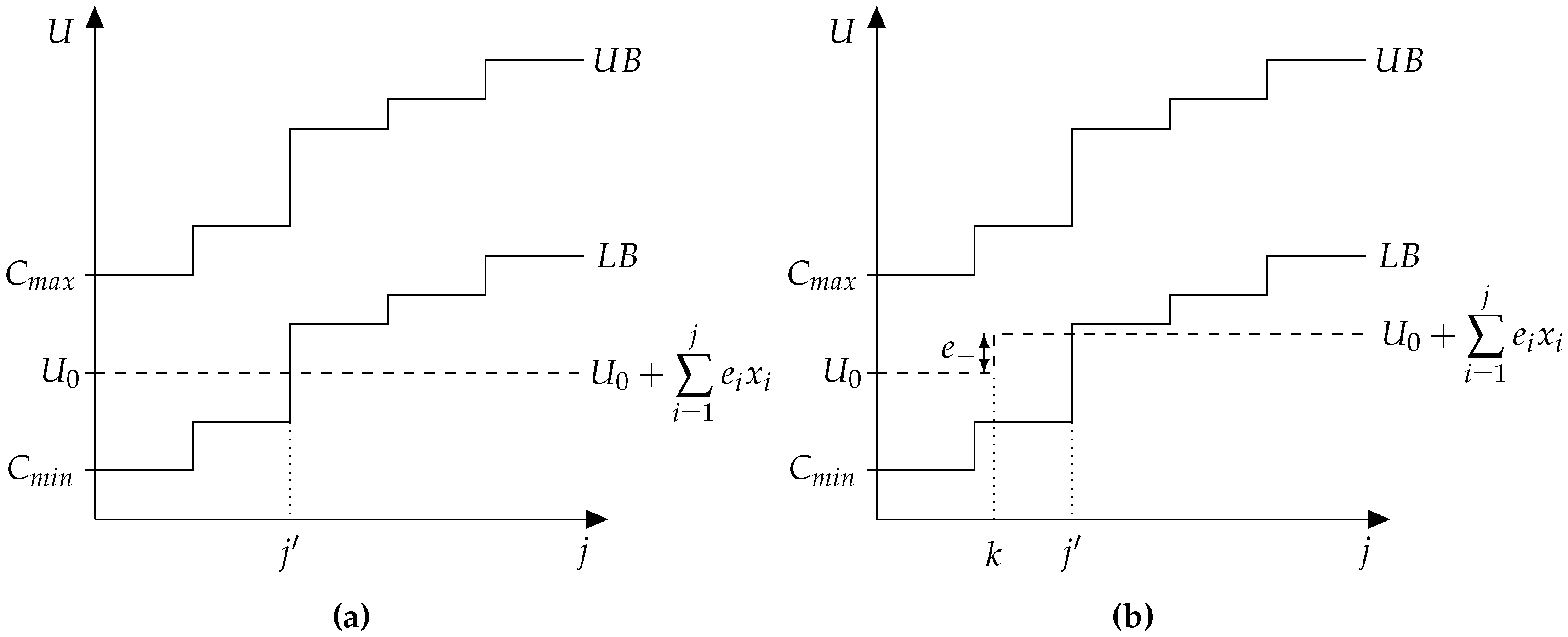
Our algorithm starts by setting all decision variables, $x_i$, to zero. It then checks at what day j the first violation (which has to be a violation of the lower bound) occurs; we call this day $j^{\prime }$. The algorithm then determines the interval in $\{1,\dots ,j^{\prime }\}$ with the lowest energy cost, interval k. If setting $x_k=1$ does not violate the upper bound, we update the solution with $x_k=1$; this process is depicted in Figure 2. The algorithm then repeats this process until the violation of the lower bound at day $j^{\prime }$ has been resolved. Subsequently, the algorithm checks where the next violation (if any) of the lower bound occurs and resolves it in the same way. This is repeated until all violations of the lower bound have been resolved.

To avoid checking the same interval multiple times, every interval is assigned a flag $f_i$ that designates whether adding this interval to the solution does not violate the upper bound. At the start, all the flags $f_i$ are set to true, denoting that all intervals can be added without violating the upper bound. While looking for the interval k with the lowest price, only intervals with $f_i=\mathrm{true}$ are considered. If it is concluded that setting $x_k=1$ would violate the upper bound, it is instead kept at $x_k=0$, and the flag $f_k$ is set to false. Furthermore, we know that if adding interval k to the solution violates the upper bound, that all other intervals before k, with the same or a larger amount of energy to be stored (i.e., the energy amount $e_i$ of that interval is larger or equal to $e_k$), will also violate the upper bound. This means we set all flags $f_i$ to false for intervals $i<k$ for which the energy amount $e_i$ during interval i is larger than or equal to the energy amount during interval k, $e_k$.

When all the violations of the lower bound have been resolved, the algorithm has found a feasible solution. However, it may be possible to find a better solution, since there may be intervals with negative energy prices that have not been used and can still be added to the solution without violating the upper bound, thus decreasing the objective value given by (2a). For this reason, the algorithm checks if there are any intervals left that have $p_i⩽0$, $x_i=0$ and $f_i=\mathrm{true}$, and adds those intervals to the solution in order of ascending energy price, as long as they do not violate the upper bound, until no such intervals remain. The entire algorithm is summarized in pseudocode in Algorithm 1. It should be noted that similar problems are discussed in the literature; for example, [23] discusses the optimization problem (2) with continuous instead of binary decision variables (problem CRA in that work).

Algorithm 1: Determine target values.

If this greedy algorithm were adapted for the LP relaxation of the optimization problem (2) (i.e., if Constraint (2f) is relaxed so that $x_i$ can be a fractional value), it would provide an optimal solution [23]. This implies that the error of our greedy algorithm is somehow related to the integrality gap of the optimization problem (2). Furthermore, it is easy to see (by an interchange argument) that the algorithm gives the optimal solution to the optimization problem (2) if $e_{-}=e_{+}$. However, in our case, where $e_{-}\ne e_{+}$, there are specific cases imaginable where our algorithm does not give the optimal solution. However, based on the relation with the integrality gap and the specific structure of the problem, we expect that for the cases considered here, the solution will be very close to optimal.

To incorporate the targets resulting from the solution of the optimization problem (2) into the ILP model described in [22], an additional term that penalizes the model for being under the target $U_j$ or rewarding the model for being over the target is added to the objective function. This term is: $-c_j(U_j^{*}-U_j)$, where $U_j^{*}$ is the amount of useful energy in the Ecovat buffer at the end of day j and $c_j$ is a positive constant. The useful energy content of the Ecovat buffer is given by Equation (3) using the temperatures in the buffer at time interval j (denoted by $T_{j,s}$). The value of $c_j$ is constant during a given day, but can be varied between days to increase or decrease the influence of the additional term on the objective function.

4. Simulation Setup

To investigate the impact of adding the target values achieved with the method described in the previous section to the rolling horizon approach described in [22], we use the same inputs as used in that paper. This means the heat demand profiles that are used are averages of historical heat demand data for the period 2005–2011. Furthermore, the energy prices used in [22] are the real Dutch energy prices from 2014; for the work presented in this paper, we ran simulations using real Dutch energy prices from 2011, 2013, 2014 and 2015 (We have omitted 2012 from this analysis. We wanted to avoid normalization issues due to 2012 being a leap year, thus having a different number of days.) to investigate the effects of various energy prices on the performance of the model. 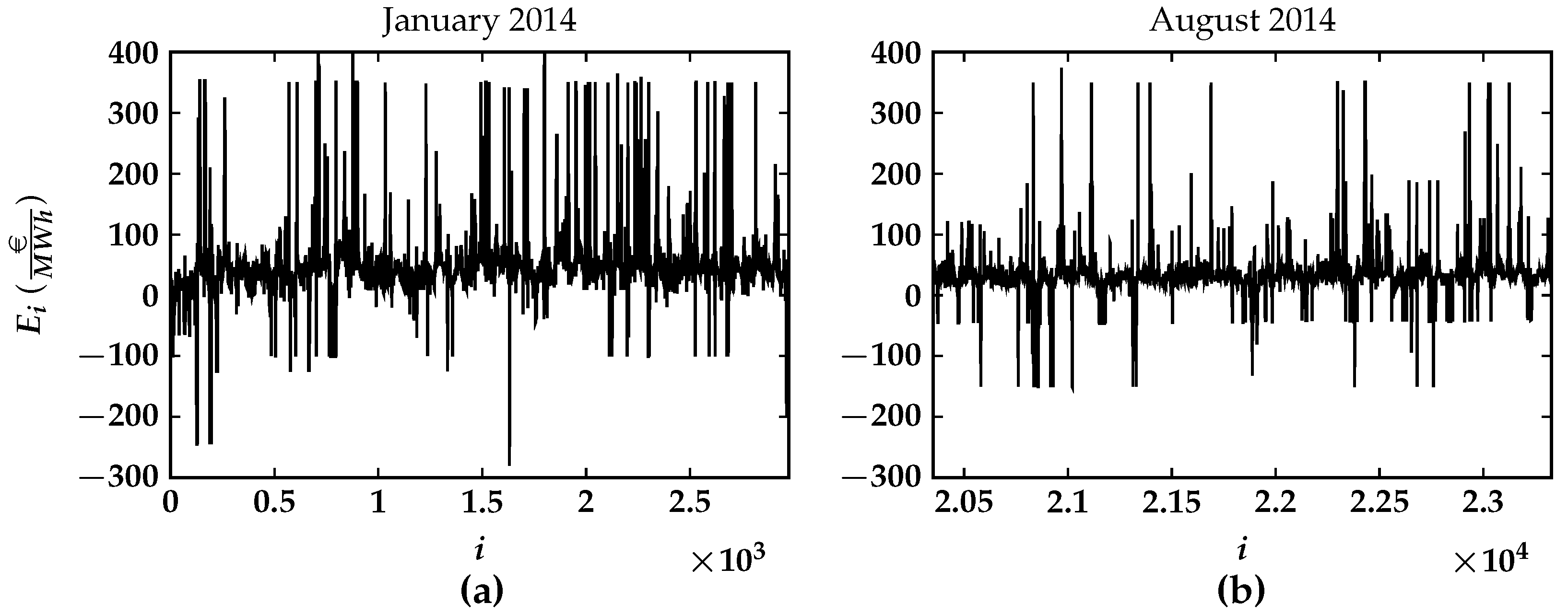Figure 3 shows the energy prices from the months of January and August from 2014. As can be seen, there is a number of intervals in both months with negative energy prices, but intervals with very high energy prices are more frequent in January, while the average price is slightly lower in August. In other words, at this point in time, there will be time intervals with negative prices throughout the entire year in which the Ecovat buffer can be (re)charged.

Where a good estimate for the expected heat demand can be made based on historical data, this is much harder for future energy prices. For this reason, we also investigate the effect of errors in energy price predictions on the achieved results. To do so, we consider two cases. In the first case, we use perfect predictions (PP) to generate the target values. In this case, we assume that all prices of the entire year are known to us beforehand. As mentioned, we have data for Dutch energy prices from a number of recent years, and therefore, we can create several instances of the problem. In the second case, we consider the other extreme, namely that we have no predictions available (NP) to generate the target values. This implies that the intervals in which energy needs to be stored get distributed equally over the entire year. In the NP case, we therefore do not require any data for energy prices. All the other input data used in both the optimization problem (2) and the ILP model from [22] are the same for both the PP and NP cases.

The weight $c_j$ in the additional term added to the objective function of the ILP model, which incentivizes the ILP model to stay above the target value, is varied from day to day, based on the difference between the target and the useful energy content of the buffer (calculated using Equation (3)) at the end of the previous day (note that the optimization problem in the ILP model is solved for each day independently). The values for $c_j$ are chosen to lie between 0.009 $(\mathrm{when}{U}_{j-1}^{*}⩾U_{j-1})$ and 0.25 $(\mathrm{when}{U}_{j-1}^{*}=0)$. These values have been determined experimentally to work well. More precisely the value of $c_j$ is then given by:

$$\begin{array}{}(7\mathrm{a})& \hfill c_j& =0.009\hfill & \mathrm{if}{U}_{j-1}^{*}⩾U_{j-1},\hfill (7\mathrm{b})& \hfill c_j& ={\left[\sqrt{0.2401}\left(1-\frac{U_{j-1}^{*}}{U_{j-1}}\right)\right]}^2+0.009\hfill & \mathrm{otherwise},\hfill \end{array}$$

which means the penalty for being under the target grows quickly when the useful energy content of the buffer drops further below the target. When the useful energy content of the buffer is above the target, the model is rewarded slightly. Different values for $c_j$ may of course be used depending on the maximum price one is willing to accept on the energy market; a value $c_j=0.009$ translates to a maximum price of $9\frac{€}{\mathrm{MWh}}$ being accepted by the ILP model. The initial ILP model presented in [22] did not include this term in the objective function. This implies that the maximum price accepted by that model was $0\frac{€}{\mathrm{MWh}}$, unless the energy content of the buffer got so low that it would be unable to supply the heat demand. In that case, the model might be forced to accept higher energy prices, as there may be no time intervals with low energy price available within its time horizon (which in that case was limited to only a few days, as discussed before). Note that this would not be necessary if the model is able to look sufficiently far ahead.

Instead of choosing the minimum and maximum values for the targets, $C_{min}$ and $C_{max}$, at 0 kWh and the buffer capacity, respectively, we choose slightly different values to allow for a ‘safety margin’. Especially for the minimum value, it seems unwise to allow a target of 0 kWh, since in this case, the ILP model could end a day with an empty buffer without punishment. If after this day, there are less opportune moments to store energy in the buffer than was predicted beforehand (i.e., energy prices are higher than expected), it could lead to unnecessarily high costs that could have been prevented by setting $C_{min}$ slightly higher. In that case, it is still possible for the model to end a day with an empty buffer; however, it will only do so if no other choice is possible (i.e., a day with only very high energy prices). For this reason, the minimum and maximum capacities, $C_{min}$ and $C_{max}$, in the optimization problem (2) are taken at 5000 kWh and 95% of the actual maximum useful energy capacity of the Ecovat buffer, respectively. Instead of choosing 5% for the minimum useful energy capacity, which would lead to a low minimum capacity for high demand temperatures, we chose 5000 kWh, which is about the energy required to satisfy the heat demand during two winter days in the instance we consider here. This value was found to work sufficiently for the cases considered in this work, since throughout the year, there are always some intervals with low energy prices. However, if long periods of time with only a few or no intervals with low energy prices are expected, a higher minimum capacity would have to be used to avoid unnecessarily high costs. This is especially important for the NP case, where such an expectation is not taken into account specifically. Even though we assume that no predictions are available for the energy prices, we might still have the expectation that during winter, a long period without negative price intervals might occur, in which case, taking a higher value for $C_{min}$ is advisable to avoid potentially high costs. The actual useful energy capacity of the Ecovat buffer, which is required to determine $C_{max}$, depends on the maximum temperature allowed in the buffer, as well as on the demand temperature. This maximum can be calculated using Equation (3) by substituting the maximum temperature allowed in segment s, $T_{max,s}$, for $T_{i,s}$. In this work, we use slightly lower values for $T_{max,s}$ than in [22]. The reason for this is that the combination of the higher maximum temperatures used in [22], the temperature ranges of the heat pumps and the division of the horizon into shorter time ranges can lead to infeasible solutions. This can happen when the model leaves the buffer in a state at the end of a day such that no feasible solution can be found for the next day. Specifically, the problem that may arise in the model used in [22] was that the temperature of the fourth segment became higher than the maximum temperature the (low temperature) heat pump could supply. If this happens and the temperature of the fifth segment is about to exceed its maximum allowed temperature, there is no way for the model to decrease its temperature due to the heat pump being unable to transfer heat from Segment 5 to Segment 4, which leads to infeasibility. To overcome this problem, we simply take a maximum temperature for Segment 4 lower than the maximum temperature the heat pump can supply (the maximum temperature for Segment 3 is lowered for the same reason). It should be noted that only one device can be connected to a given segment during a time interval. This means for example that we cannot simultaneously connect the high temperature heat pump to transfer heat from Segment 4 to Segment 3 while using the low temperature heat pump to transfer heat from Segment 5 to Segment 4. Because of this, we use $T_{max,s}=\{90,90,78,48,5\}$ in this work, while $T_{max,s}=\{90,90,90,90,5\}$ was used previously. To check if these changed maximum temperatures have a significant influence on the results, the optimizations from [22] were rerun using the new values for $T_{max,s}$ instead of the values used there. The difference in results found was negligible (less than 0.1% difference in objective values).

The values for the maximum energy storable during an interval at a negative or positive energy price, $e_{-}$ and $e_{+}$ respectively, depend on the amount of energy generated by the heat pumps and resistance heater (only in the case of $e_{-}$) on average. The amount of energy the resistance heater contributes to $e_{-}$ is easy to determine because of its constant coefficient of performance of one. However, the contribution of the heat pumps is much harder to determine. Their contribution depends on the demand temperature $T_d$, the temperatures inside the buffer $T_{i,s}$, the temperature ranges of the heat pumps and their coefficients of performance. This implies that these values are dependent on the current state of the buffer and that therefore $e_{-}$ and $e_{+}$ can only be rough estimates. For this reason, we also investigate the effect of various estimates of these parameters on the results of the model. To this end, we use three estimates for $e_{-}$ and $e_{+}$, a low estimate (LE), a medium estimate (ME) and a high estimate (HE). These estimates are given in

Table 1. Table showing values of $e_{-}$ and $e_{+}$. LE, low estimate; ME, medium estimate; HE, high estimate.

	${\mathit{e}}_{-}$ (kWh)	${\mathit{e}}_{+}$ (kWh)
LE	256	6
ME	262	12
HE	268	18

. For the results presented in the next section, the medium estimate is used, unless specified differently. It should be noted here that when estimating these values, we make the assumption that the resistance heater is only used to store energy when the energy price is non-positive, which is not necessarily true depending on the values of $c_j$. This assumption is also evaluated in the next section. The differences in the estimates for $e_{-}$ are relatively small because the contribution of the resistance heater, which supplies by far the largest portion of the energy during intervals with negative energy prices, is easily estimated as mentioned before. While the estimates for the heat pumps are much more uncertain, they supply a much smaller portion of the energy during such times, leading to small relative differences.

In the model described in [22], the criteria to stop the solver during a given step (in this case, a day) are where when the gap between the best bound and the best solution found was less than 0.2% or if the solver took more than an hour to reach this condition. Here, we add a third criterion, namely that the solver also stops when the gap between the best bound and the best solution found is less than 1 €.

5. Results

By solving the optimization problem (2) using the method described in Section 3, we obtain a target for the useful energy content of the Ecovat buffer at the end of every day within the optimization horizon. First, we wish to investigate whether the choice we made for the NP case, namely that we distribute the amount of intervals in which storing energy is required evenly throughout the year, leads to target values that are close to those obtained from the PP case. In Figure 4, the resulting target values are shown for a demand temperature of 40 ${}^{°}$C for the PP case when using real Dutch energy prices from the years 2011, 2013, 2014 and 2015, as well as for the NP case (which is the same for every year). The targets for the PP case using energy prices from 2013 or 2015 have a similar shape as the targets for the NP case. However, the targets for the PP case using energy prices from 2011 or 2014 are significantly different from the targets for the NP case. This means the choice to distribute the number of intervals in which energy needs to be stored equally over the year seems reasonable for the years 2013 and 2015, but leads to significantly different targets for the years 2011 and 2014 compared to the PP case. This is due to the uneven spread in energy prices in 2011 and 2014, while the NP case assumes a fairly even spread throughout the year.

Figure 5 shows the same type of results for the PP and NP cases; however, this time for a demand temperature of 60 ${}^{°}$C. Similarly to Figure 4, the targets for the PP case using energy prices from 2013 or 2015 have a similar shape compared to the targets for the NP case, while the targets for the PP case using energy prices from 2011 or 2014 are significantly different. The largest difference between Figure 4 and Figure 5 is that in the second case (with a demand temperature of 60 ${}^{°}$C), the buffer is almost completely depleted at the end of winter or during spring, except for the PP case using energy prices from 2014, while in Figure 4, this only occurs for the PP case using energy prices from 2011. That the buffer is almost completely depleted for most years in the higher demand temperature case is due to the fact that the amount of energy demanded stays the same (compared to the lower demand temperature case), while the initial amount of useful energy in the buffer is much lower for the same initial temperature distribution due to the higher demand temperature.

From the previous figures, we have seen that the PP and NP cases can lead to target values that differ significantly between those two cases. Next, we investigate whether this difference in target values also leads to a difference in the results of the ILP model. In Figure 6, the results of the optimization with a demand temperature $T_d$ = 40 ${}^{°}$C without targets are compared with optimizations using the long-term planning described in this paper. The various lines in the figure indicate the temperature in the corresponding segment of the buffer. If at least one of the lines is above the demand temperature, then there is useful energy left in the buffer. As already observed in [22], the optimization without long-term planning does well in this case, as there is always enough energy to supply the requested heat demand. In this case, adding a long-term planning (both in the PP and NP cases) has the effect of a larger amount of useful energy being present in the buffer throughout the year, which is shown in the figure by the temperatures in the buffer being higher throughout the year. However, this leads to a slight decrease in the objective value (note that the objective is to minimize costs, so a negative objective value means a profit has been made) of the ILP as shown in

Table 2. Table comparing optimizations using energy price data from 2014 and $T_d$ = 40 ${}^{°}$C.

	Objective Value (€)	${\mathit{U}}_{{\mathit{N}}_{\mathit{i}\mathit{n}\mathit{t}}}$ (kWh)
No targets	−28,131	74,402
PP	−27,252	126,278
NP	−27,228	126,244

, due to the slightly higher energy prices that are accepted by the model including targets. As discussed in the previous section, the model without targets accepts only negative prices, while the model with targets will also accept some amount of positive price intervals, depending on the value of $c_j$. The higher objective value for the model that includes targets is compensated by the higher useful energy content of the buffer at the end of the optimization, due to the safer strategy used by adding these targets. Even though in this case, it would be possible to not include a long-term planning step in the model, and still obtain good results, we find that the differences are small. As these differences are only small, it is still advisable to incorporate targets in order to employ a safer charging strategy. The reason for this is that not including targets in cases they would be beneficial may lead to a large decrease in profit, while including targets when not strictly necessary only leads to a slight decrease in profit. It should be noted that the differences between the PP and NP cases are very small for the optimization shown in Figure 6 and Table 2 (less than 1% in objective value).

While the model without a long-term planning step performs well for the case with a demand temperature of 40 ${}^{°}$C, it is shown in [22] that this is no longer the case when the demand temperature is increased to 60 ${}^{°}$C. In Figure 7, the results are shown for a demand temperature of 60 ${}^{°}$C. In this case, the optimization without a long-term planning step performs very poorly as was already observed in [22]. The addition of a long-term planning step makes a large difference in this case. As can be seen, there is always enough useful energy in the buffer to be able to supply the heat demand. Furthermore, the amount of useful energy in the buffer at the end of the optimization is a lot higher compared to the case when no long-term planning step is used.

Table 3. Table comparing optimizations using energy price data from 2014 and $T_d$ = 60 ${}^{°}$C.

	Objective Value (€)	${\mathit{U}}_{{\mathit{N}}_{\mathit{i}\mathit{n}\mathit{t}}}$ (kWh)
No targets	−27,705	303
PP	−27,409	47,901
NP	−26,949	58,243

shows the objective values and the amount of useful energy in the buffer at the end of the optimization for the various cases. When a demand temperature of 60 ${}^{°}$C is used, it is clear that the addition of a long-term planning step to the ILP model leads to a large improvement in the results. Again, we see that the differences between the PP and NP cases are small (less than 2% in objective value).

In Figure 6 and Figure 7, there seems to be little difference in the results when comparing the PP and NP cases. To get some more insight regarding this behavior, we investigated if this stays the same for the other years: 2011, 2013 and 2015. The corresponding results are summarized in

Table 4. Table comparing optimizations using energy price data from different years and $T_d$ = 60 ${}^{°}$C.

	Objective Value (€)	${\mathit{U}}_{{\mathit{N}}_{\mathit{i}\mathit{n}\mathit{t}}}$ (kWh)
2011 PP	−21,506	89,562
2011 NP	−21,250	89,856
2013 PP	−41,290	52,442
2013 NP	−40,850	61,824
2014 PP	−27,409	47,901
2014 NP	−26,949	58,243
2015 PP	−47,754	66,300
2015 NP	−47,753	68,899

. We can see that for all the years considered, the PP and NP cases give very similar results. The largest relative difference is observed for 2011, but even there, the difference in the objective value is less than 2%. In Table 4, only the results for a demand temperature of 60 ${}^{°}$C are shown. However, the results obtained for a demand temperature of 40 ${}^{°}$C show the same behavior, namely that the differences between the PP and NP case results are very small. The NP case gives slightly higher objective values, but also has higher useful energy values at the end of the optimizations to compensate for this. Whether this trade-off is worthwhile depends on the expected energy prices after the optimization horizon.

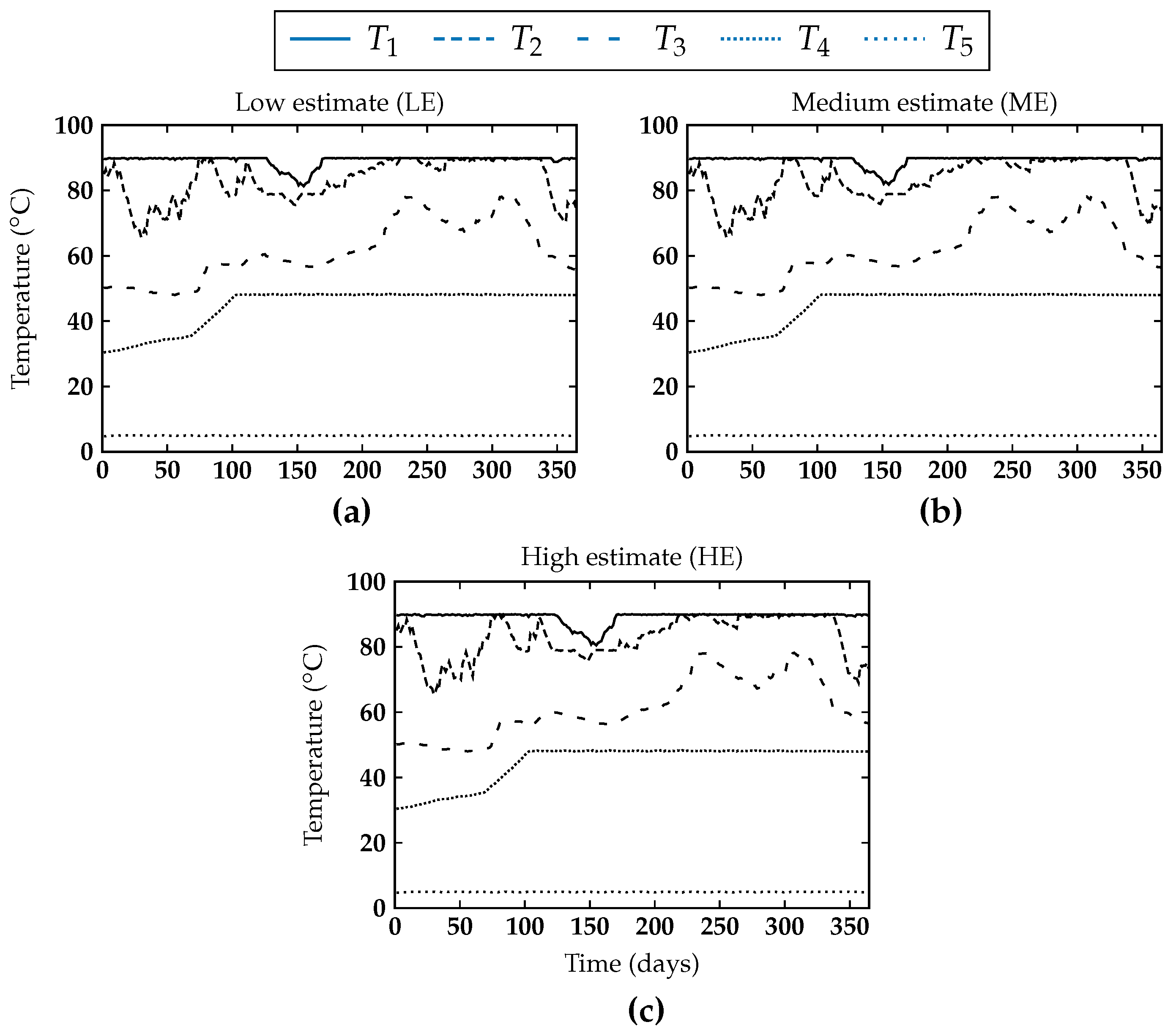
Finally, we investigated the influence of the choice for $e_{-}$ and $e_{+}$ on the results. These values were defined as the amount of energy that gets stored in the Ecovat buffer in one time interval, for negative and positive energy prices, respectively, if the optimization decides to use an interval to store energy in the Ecovat buffer. At the end of the previous section, we specified low, medium and high estimates for these values. We again take the energy prices from 2014 and a demand temperature of 60 ${}^{°}$C and compare the effect of the different estimates for $e_{-}$ and $e_{+}$. The results of this comparison are presented in Figure 8 and

Table 5. Table comparing optimizations using energy price data from 2014, $T_d$ = 60 ${}^{°}$C and different estimates for $e_{-}$ and $e_{+}$.

	Objective Value (€)	${\mathit{U}}_{{\mathit{N}}_{\mathit{i}\mathit{n}\mathit{t}}}$ (kWh)
LE	−27,391	48,589
ME	−27,409	47,901
HE	−27,448	46,819

. As can be seen, the results are again very similar. The higher the estimates for $e_{-}$ and $e_{+}$, the lower the objective value (more profit), but the lower the amount of useful energy in the buffer at the end of the optimization. This comparison was also carried out using energy price data from the other years, yielding similar results to those shown in Figure 8 and Table 5.

We observe that different values for $e_{-}$ and $e_{+}$ give very similar results and, more generally, that two sets of target values that differ significantly (for example the NP and PP cases for 2014 shown in Figure 7 and Table 3) still give very similar results. This leads us to believe that the simplifying assumption we made at the end of Section 4, namely that for determining $e_{-}$, we assume the resistance heater only runs when the energy price is non-positive, has a negligible effect on the results of the optimizations presented here.

The presented results show that the addition of a long-term planning step to the ILP model is robust against prediction errors. The results show that adding long-term planning to the model improves the results, while being only slightly influenced by differences in energy prices. This means that as long as the ILP model is given target values that are somewhat close to the actual prices, i.e., if they follow the expected seasonal behavior (for example, a high target at the end of summer), the results of the ILP model will differ at most a few percent. However, if as a consequence of the energy transition, the prices will get more volatile in the future, it may become more important to have good predictions of these prices to still obtain good results. This result can be explained by taking a closer look at the energy prices. In Figure 9, the energy prices from 2014 are plotted after sorting from lowest to highest. There are some very low prices, which the model will always try to use, and some very high prices, which the model will always try to avoid. However, between those extremes, there are many prices that differ only slightly from each other. This means that even if the ILP model is given targets that are suboptimal, thus unnecessarily selecting some intervals with a higher price, the difference in objective value will be very small.

6. Conclusions

In this paper, we have presented the addition of a long-term planning step to the ILP model to control an Ecovat buffer described in [22]. We demonstrated that adding a long-term planning step greatly improved results for the case in which a demand temperature of 60 ${}^{°}$C was used.

Additionally, we showed that the extended model is very robust against prediction errors in the energy prices. The ILP model gives similar results even for target values that differ significantly from each other (less than 2% difference in objective value in the worst case and often much smaller differences were observed).

Finally, we investigated the effect of changing the values of $e_{-}$ and $e_{+}$, which represent an estimate of the amount of energy that gets stored in one time interval, since the contribution of the heat pumps to the value of these parameters is difficult to estimate. However, we found that the results are very similar.

In conclusion, we find that as long as the targets supplied to the ILP model are not too different from reality (in other words, if they follow the expected seasonal behavior), the results of the model will not differ significantly. In future work, we aim to simplify the Ecovat model while retaining an acceptable level of accuracy. This is important when doing operational planning to control a real Ecovat system in the future. Furthermore, a simpler model would allow us to integrate an Ecovat system into a larger demand-side management simulation of a neighborhood. Additionally, an interesting avenue for future research would be to consider some type of forecasting of energy prices, for example using a stochastic model, instead of just looking at the extreme cases (PP and NP) considered in this work. Finally, while we have considered the effect of prediction errors in energy prices, we have not done so for prediction errors in heat demand or weather data. We expect the model to be robust against these as well, since supplying the ILP model with slightly different targets does not change the results significantly. Even in harsh winters, we expect the targets to remain very similar, the main difference will probably be that more energy will have to purchased on the energy market, thereby lowering profits. However, it would be interesting to consider prediction errors in heat demand and weather data in future work to confirm whether this expectation is correct.