Harmonic Analyzing of the Double PWM Converter in DFIG Based on Mathematical Model

1
Key Laboratory of Magnetic Suspension Technology and Maglev Vehicle, Ministry of Education, Southwest Jiaotong University, Chengdu 610031, China
2
School of Electrical Engineering, Southwest Jiaotong University, Chengdu 610031, China
*
Author to whom correspondence should be addressed.
Energies 2017, 10(12), 2087; https://doi.org/10.3390/en10122087
Submission received: 20 October 2017
/
Revised: 18 November 2017
/
Accepted: 5 December 2017
/
Published: 8 December 2017
Abstract
:Harmonic pollution of double fed induction generators (DFIGs) has become a vital concern for its undesirable effects on power quality issues of wind generation systems and grid-connected system, and the double pulse width modulation (PWM)converter is one of the main harmonic sources in DFIGs. Thus the harmonic analysis of the converter in DFIGs is a necessary step to evaluate their harmonic pollution of DFIGs. This paper proposes a detailed harmonic modeling method to discuss the main harmonic components in a converter. In general the harmonic modeling could be divided into the low-order harmonic part (up to 30th order) and the high-order harmonic part (greater than order 30) parts in general. The low-order harmonics are produced by the circuit topology and control algorithm, and the harmonic component will be different if the control strategy changes. The high-order harmonics are produced by the modulation of the switching function to the dc variable. In this paper, the low-order harmonic modeling is established according to the directions of power flow under the vector control (VC), and the high-order harmonic modeling is established by the switching function of space vector PWM and dc currents. Meanwhile, the simulations of harmonic a components in a converter are accomplished in a real time digital simulation system. The results indicate that the proposed modeling could effectively show the harmonics distribution of the converter in DFIGs.
1. Introduction
The installation rate of renewable energy sources is increasing rapidly in large power plants [1,2], and the fastest growing source of renewable energy in the power industry is wind energy [3]. Many studies have been done to analyze the different kinds of problems in wind turbines after connecting to the grid [4,5,6,7,8]. In regards to wind power generation, the double fed induction generator (DFIG) has become the leading type of wind turbines. As a variable speed wind generator, DFIG has many advantages compared with other types, such as its good stability after connecting to the grid, and decoupled control of active and reactive power [9,10,11]. These advantages are realized on the basis of the pulse width modulation (PWM) converter, which is widely used in the DFIG systems for its ability to realize a bidirectional flowing of energy. As a power electronic device, the double PWM converter acts as a major harmonic source in DFIGs. Unlike other harmonic sources of conventional power grids, the harmonics in the converter will cause voltage fluctuation after connecting to the grid, which could affect the accuracy of the automatic devices and result in a poor power quality [12].
With the increase of the DFIGs installation rate, the converter harmonics of converter are becoming an issue that must be solved. Many studies have been done to analyze the generation mechanism of the harmonics in DFIGs [13,14,15]. Aiming at the disadvantage of the narrow application range of various harmonic models, a unified model of DFIG was proposed by Fan et al. [14], which was also effective with harmonic input from the rotor. Abniki et al. proposed a DFIG harmonic model that can precisely analyze the power quality even if the harmonic distortion exists [15]. However, many papers focus on the whole model of the DFIG, which is only good for a macro analysis of actual harmonic components. Most of them do not relate to the analysis of the converter in the DFIG, and don’t give a detailed harmonic derivation with the consideration of the control methods. The harmonic modeling established in this article focuses on the converter of the DFIG, considering the influence of the different control methods and the different operation states, and is relatively complete for the study of the harmonics. In addition, this detailed harmonic modeling also has laid a relatively sound foundation for the future research on the influence of other factors.
The difficulty of the harmonics analysis in a converter is that the power flow directions and the control strategies of grid side converter (GSC) and rotor side converter (RSC) are very different [16], which have an important impact on the generation of harmonics. There are many studies on the control strategy of the converter. The most commonly used control method is vector control (VC) [17,18,19], which has some advantages, such as precise steady-state performance, less power ripple, and lower converter switching frequency. In this paper, the harmonic modeling will be carried out under the VC, and the modeling will take into account the differences of power flow and specific control strategy in GSC and RSC. The proposed harmonic modeling proposed in this paper consists of two parts, the low-order harmonic modeling and the high-order harmonic modeling. These two models can be derived by their influence factors. The low-order harmonic component is affected by the control strategy and circuit topology, and the high-order harmonic component is affected by the modulation of the dc variable by the switching function [20,21,22], so the order of high harmonics will occur near the frequency modulation ratio, and the boundaries of high-order and low-order harmonics should be defined below the frequency modulation ratio. The frequency modulation ratio in this article is set to be 40, so it can be defined that the order of high harmonic is greater than 30, and the order of low harmonic is from 2 to 30. A complete and detailed harmonic modeling can be established through the above derivation method. From this modeling, the influence of the control method on the harmonic generation mechanism can be clearly shown, and we can conduct follow-up research based on this modeling.
The rest of this paper is organized as follows: in Section 2, the mathematic modeling of the converter in DFIG is deduced, which is divided into the low-order harmonic modeling and the high-order harmonic modeling. In Section 3, the simulations of the harmonic modeling are accomplished, which verify the correctness of the harmonic modeling. In the last part, the results of the whole harmonic modeling are summarized.
2. Harmonic Modeling of Double PWM Converter
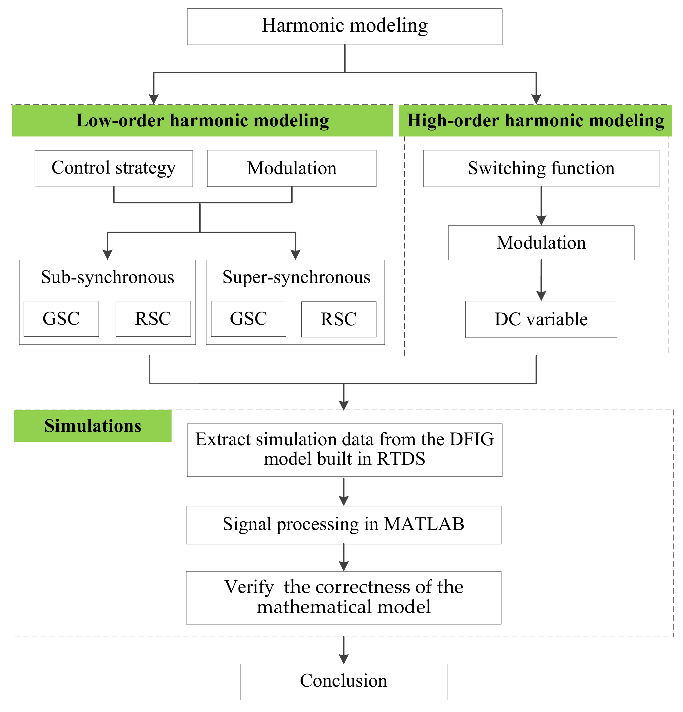
The dual PWM converter is a kind of power electronic device, which is characterized by a non-sinusoidal current consisting of severe harmonic components. The proposed mathematic modeling can analyze these harmonic components of the converter in detail. The whole idea of harmonic modeling is described in Figure 1.
2.1. Low-Order Harmonic Modeling
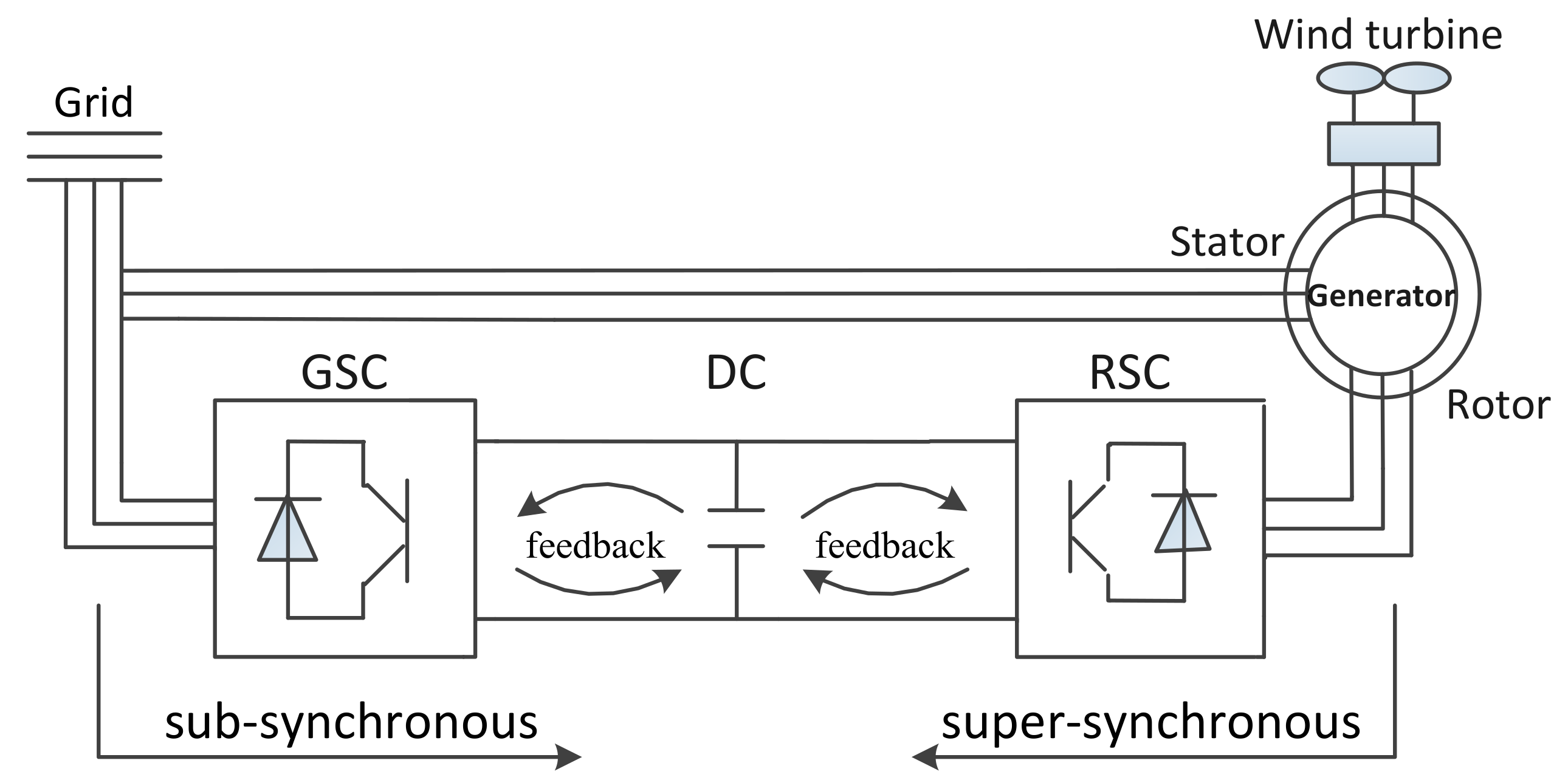
Since the low-order harmonics are produced by the circuit topology and control algorithm, the harmonic generation will be different for different control strategies. The control strategy used in this paper is VC, which includes RSC control and GSC control, and there will be some differences between them in sub-synchronous state and super-synchronous state. Therefore, the harmonic modeling is mainly classified into three parts, the low-order harmonic modeling of GSC in sub-synchronous state, the low-order harmonic modeling of RSC in super-synchronous state and the low-order harmonic modeling of the inverter. The inverter part includes the low-order harmonic modeling of RSC in sub-synchronous state and GSC in super-synchronous state. The power conversion in the two states is shown in Figure 2.
2.1.1. The Low-Order Harmonic Modeling of GSC in Sub-Synchronous State
As shown in Figure 2, when the motor is running in sub-synchronous state, the GSC operates as a rectifier and the energy will be sent from the grid to the rotor. In this direction of power flow, the control strategy of GSC is the double closed loop control that includes current inner loop and voltage outer loop [23], which is derived through the conversion of the voltage and current to the d and q axial component [24,25]. The dq decoupled control of GSC is shown in Figure 3, where uga, ugb and ugc mean the phase voltage of grid, and the voltage Ug is a space vector. iga, igb and igc mean the phase current of the input GSC, and the current Ig is space vector. uca, ucb and ucc are the ac phase voltage of converter, and the voltage Uc is a space vector.
The voltage Udc is the dc voltage of the output GSC. The current idc is the dc current of the output GSC. il is the load current. ic is the capacitance current. igd and igq mean dq axis grid currents. ugd and ugq mean the dq axis grid voltages. ω1 is the reference frame speed. 3s/2s mean the transformation from the three-phase A, B, C axis to the two-phase stationary αβ axis, and 2s/2r mean the transformation from the two-phase stationary αβ axis to the two-phase rotation dq axis.
The voltage outer loop is designed to make the dc link voltage udc and the d axis current component igd constant, and the current inner loop is designed to modulate the grid power factor.
As shown in Figure 3, the energy is sent from the grid to the rotor, and then one part will be input to the grid side through feedback loop to regulate power factor. The input power of GSC is expressed as
Since the harmonic modeling in this article is proposed under the ideal output condition, it can be assumed that the input current and voltage from grid only contain the fundamental component and the harmonic components that have an integer multiple of the fundamental frequency.
where Ugk and Igk are the effective value of the kth harmonic content of grid voltage and grid current. Φ means the angle between the grid fundamental voltage and current, and ϕk means the angle between the kth voltage and the current harmonic. Because the amplitudes of the grid harmonic components are too small relative to the fundamental component, the interaction between the grid voltage and current harmonics can be neglected. Thus, the input power of GSC can be written as:
As shown in Equation (3), the input power of GSC consists of two parts, where UgIgcosϕ is the steady state component, and the rest parts are the dynamic components. According to the equivalent mathematical model of GSC, the output power can be expressed as
where and are the average and fluctuating values of dc voltage, and is the average value of load current . stand for the average values of the resistance. Assuming that GSC is composed of ideal switching devices, there will be no power loss in commutation, and then
In addition to the fundamental component, the harmonics caused by the interaction of grid voltage and current harmonics are calculated as 0 because of three-phase symmetry. Thus, the dc output voltage only contains the fundamental component. It is fed back into the grid current as shown in Figure 3. The dq current inner loop control of GSC can be shown as in Figure 4.
And the voltage outer loop is written as
where and stand for the proportional and integral factor of the voltage outer control loop.
The grid current can be calculated as
The mathematical modeling of the low-order harmonics of GSC in sub-synchronous state is derived by power conservation, and the harmonics are caused by the feedback from the dc link. According to the Equation (9), it can be seen that the grid current only contains the fundamental component. In the actual situation, the dc link should have the ripple components caused by the AC component from the output of RSC, but our research at this stage has not come to this point. We will increase the impact variables of the research and improve the relevant models in future research.
2.1.2. The Low-Order Harmonic Modeling of RSC in Super-Synchronous State
When the motor is running in super-synchronous state, the RSC operates as a rectifier and the energy will be sent from the rotor to the grid. The control strategy of RSC used in this paper is the double closed loop control that includes current inner loop and power outer loop [23], as shown in Figure 5.
Where ird and irq mean the dq axis rotor currents. Ls, Lr and Lm are the stator leakage, rotor leakage and magnetizing inductance. Us is the stator voltage. Ps and Qs are the active and reactive power, and ωslip = ω1 − ωr. The control is designed to make the rotor speed constant by adjusting the rotor currents, and then the output power can be kept stable. As shown in Figure 5, the input currents of RSC can be obtained as:
where ira, irb and irc mean the phase current of rotor side, and the current Ir is a space vector. Irk is the effective value of the kth harmonic content of the rotor current.
In order to simplify the original mathematical model to adapt to the implementation of linear control strategy, the rotor current expressions in Equation (10) should be calculated into the dq axis current components by coordinate transformation. The transformation matrix can be expressed as follows:
After the coordinate transformation, the rotor current expressions can be converted to the dq components under the synchronous rotation coordinate system, and the Equation (10) can be calculated as
The rotor and stator voltage expressions of DFIG can be obtained by the circuit topology as
where usd and usq mean the dq axis stator voltages. sd and sq are the dq axis stator flux vector. rd and rq are the dq axis rotor flux vector.
In the synchronously rotating reference frame, the d axis is oriented in the direction of the stator voltage vector. Because the stator is directly connected to the grid, the stator voltage will be equal to the grid voltage, so the dq axis stator voltages are
When the grid voltage is constant, the stator flux vector s can also be regarded as unchanged drq/dt = 0and dsq/dt = 0. If the stator resistance of the DFIG is ignored, the Equation (13) is substituted into the stator voltage (Equation (14)) as:
According to the Equation (16), the dq axis stator current and the stator power equations are
And the power outer loop control can be written as
where kPP and kPI mean the proportional and integral factor of the active power. kQP and kQI mean the proportional and integral factor of the reactive power.
And the RSC currents are
According to the deduced mathematic modeling of this part, it can be found that the rotor current contains only the fundamental component with an offset, and the offset is the angle between the rotating coordinate system and the stationary coordinate system.
2.1.3. The Low-Order Harmonic Modeling of the Inverter
The power flow of the inverter in two states is measured from the dc link to the ac side, and the low-order harmonics of the inverter are primarily produced by the modulation strategy. The modulation strategy used in this paper is space vector pulse width modulation (SVPWM). Comparing with other control methods, SVPWM has some advantages, such as linear operation range and higher utilization rate on the dc voltage.
In this part, the harmonic modeling of inverter is deduced based on the Fourier double integral transformation. Any time varying waveform can be expressed as an infinite series of sinusoidal harmonics after Fourier decomposition [26,27,28], and the standard expression of output phase voltage of inverter can be obtained as
where ck is the amplitude of the kth harmonic component.
The order of harmonics in this waveform can be determined by calculating the amplitude of each harmonic. For the calculation of the amplitude, the most effective approach is to rearrange ck into the double integral Fourier form Cmn.
We define Cmn as
where F(x, y) means the waveform of a basic cycle. ωc and ω0 are the are angular frequency of triangular wave and sine wave.
This function should be applied to any resonant frequency [mωc + nω0] for SVPWM. Considering only the low-order harmonic components, the waveform can be expressed in sinusoidal harmonic component as
According to the internal and external integral limit of SVPWM control, B0n is calculated as 0, and the amplitude of baseband harmonics A0n can be calculated as
Assuming the amplitude of fundamental be 1, the values of are calculated as listed in Table 1.
According to the data in Table 1, there are 3th, 5th, 7th, 9th, 15th and 17th order harmonics in the output voltage. For the output line current, the difference in the order of harmonics is the 3rd order harmonics and their multiples, which will cancel each other out in the output line current. Assuming the amplitude of fundamental is 1, the amplitude of current harmonics A0c can be shown in Table 2.
According to the data in Table 2, there are 5th, 7th, 17th order harmonics in the output line current.
2.2. High-Order Harmonic Modeling
Different from the cause of low-order harmonics, the high-order harmonics of the converter are generated by the modulation of the switching function to the dc variable, so the mathematic modeling of high-order harmonics is deduced only by the circuit structure and the switching function [29]. Since the rectifier and inverter have the same mathematical form, so their high-order harmonics can be analyzed together.
The switching function of PWM converter is defined as sa, sb, sc. In the ideal case, the dc voltage and ac current of the rectified part will satisfy the following conditions
where sua, sub and suc are the switching function of phase voltages. sia, sib and sic are the switching function of phase currents.
As shown in the derivation of low-order harmonics, the dc output voltage only contains the fundamental component. It can be obtained by
The switching function of SVPWM [30] is listed below
where Jn means the Bessel function, N is the frequency modulation ratio and N = ωc/ω0. M is the fundamental modulation depth and M = U0/Uc.
Calculating the data of the Bessel function, the fitting curve is shown in Figure 7.
According to Equations (27) and (28) and the second term of Equation (26), the high-order harmonic modeling of phase current can be derived as
(1) When m = 1 and n = 2, 4, 8, 10
Calculating the amplitude of each item, it can be obtained that there are N + 2th and N + 4th order harmonics in a phase current.
(2) When m = 1 and n = −2, −4, −8, −10
Calculating the amplitude of each item, it can be obtained that there are N − 2th and N − 4th order harmonics in a phase current.
(3) When m = 2 and n = 1, 5, 7, 11, 13
Calculating the amplitude of each item, there are 2N + 1th, 2N + 5th and 2N + 7th order harmonics in a phase current.
(4) When m = 2 and n = −1, −5, −7, −11, −13
It can be obtained that there are 2N − 1th, 2N − 5th and 2N − 7th harmonics in phase current.
According to the above equations, the high-order harmonics of the converter are associated with the frequency modulation ratio, and the orders of harmonics are N ± 2, 4, 2N ± 1, 5, 7, 3N ± 2, 4 and so on.
3. Simulations and Experimental Results
The proposed modeling of harmonics is simulated in real time digital simulation (RTDS). RTDS is a very widely used simulation device around in the world. Compared with other simulation software, RTDS has many advantages of faster calculation speed and the interactivity with practical equipment [31,32,33]. The software platform of RTDS is the real time simulator CAD (RSCAD), and the DFIG model is built in RSCAD software firstly. Then the simulation data is obtained by the operation after connecting RSCAD and RTDS. The simulation process of harmonic modeling in RTDS is shown in Figure 8.
Based on the circuit topology of DFIG, a detailed modeling of double PWM converter can be established in RSCAD. In this modeling, the fundamental modulation depth is set to be 1, and the frequency modulation ratio is set to be 40.
As shown in Figure 8, after the operation of RTDS, the obtained simulation waveforms are still need to be discussed, so it is necessary to analyze the data using the appropriate algorithm in matrix and laboratory (MATLAB). After importing the simulation data into MATLAB, the harmonics of GSC and RSC can be obtained as follows.
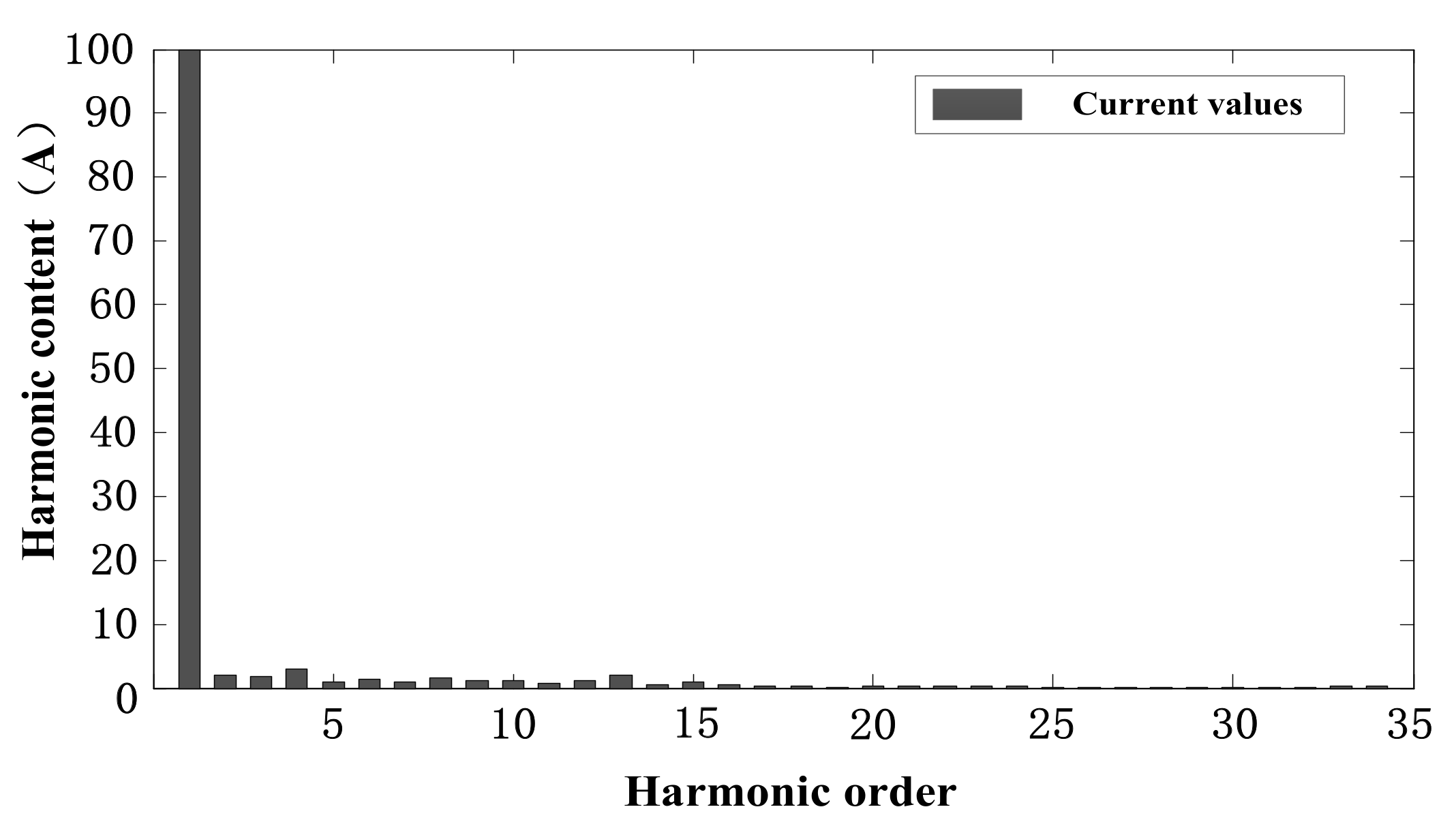
3.1. The Low-Order Harmonics of GSCin Sub-Synchronous State
The amplitude () of the current fundamental is 200 A. According to Figure 9, it can be found that there is almost no low-order harmonics in sub-synchronous state, and the simulation resultsalso verify the correctness of the low-order harmonic model of GSC.
3.2. The Low-Order Harmonics of RSCin Sub-Synchronous State
The voltage harmonics are shown in Figure 10.
The rotor current harmonics are shown in Figure 11.
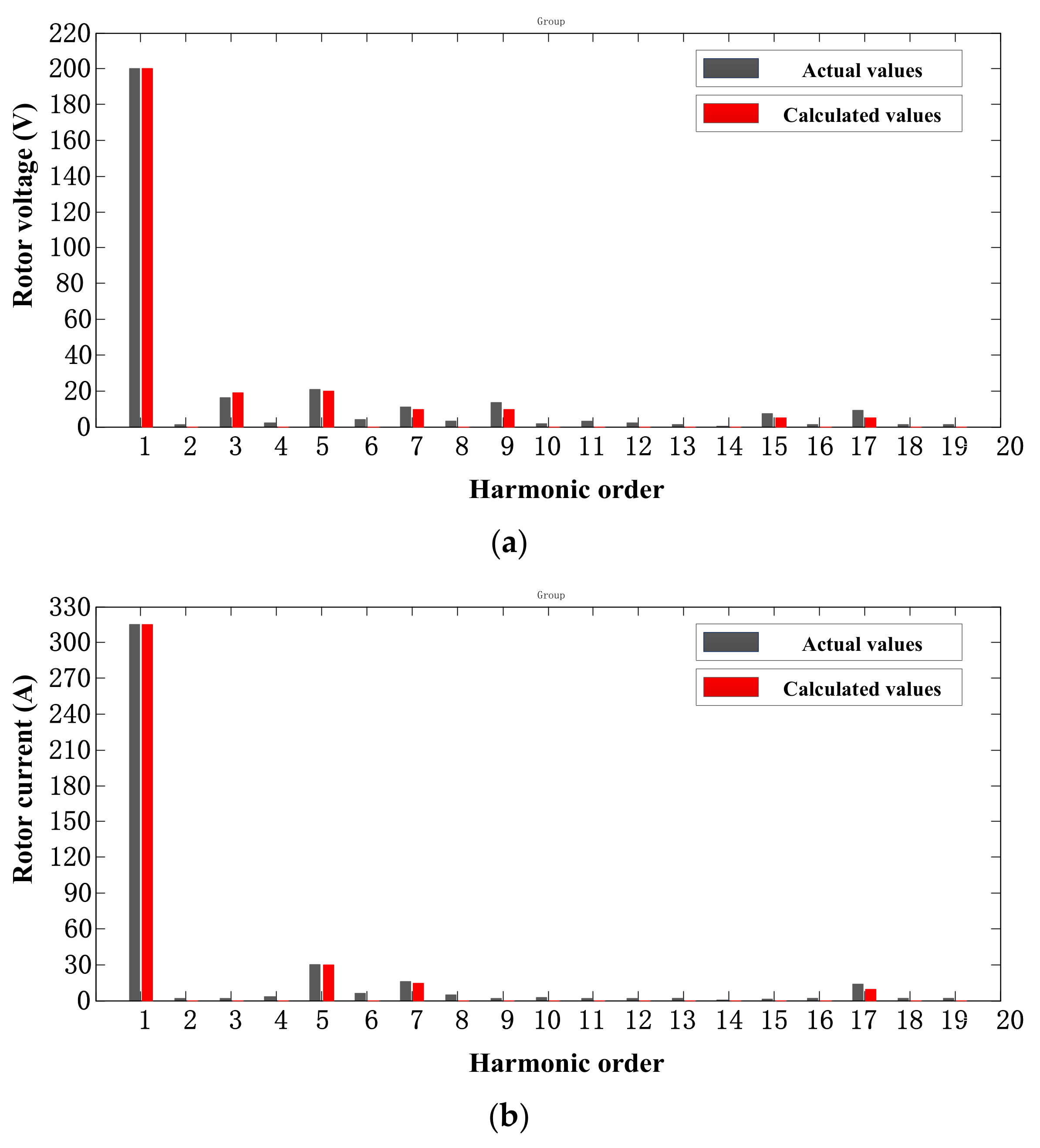
According to Figure 10 and Figure 11, it can be seen that there are 3th, 5th, 7th, 9th, 15th and 17th order voltage harmonics of RSC in sub-synchronous state, and the harmonic order of line currents are 5th, 7th, and 17th. The calculated data in Table 1 and Table 2 with the simulation data is compared in Figure 12.
The calculated values (A0nc) and the actual values (A0na)of the voltage harmonics are listed in Table 3, and the calculated values (A0cc) and the actual values (A0ca)of the current harmonics are listed in Table 4, where the amplitude (A01) of the voltage fundamental is 315 V, so the difference between the actual value and the calculated value can be calculated, , and .
According to Table 3 and Table 4, as the order of harmonics increases, the percentage of the difference between the calculated and the actual values increases gradually, but it can be seen that the percentage of the difference compared with fundamental does not exceed 2%, so in the view of the whole modeling, the derivation of harmonic order is basically correct. However, this modeling is still insufficient in the derivation of the amplitude of the harmonics which greater than order 9, the reason is most likely that this modeling is established on the ideal state. Some external factors will be considered in the next step, and the model will also be improved in future studies.
3.3. The Low-Order Harmonics of RSC in Super-Synchronous State
According to Figure 13, the current of RSC only contains the fundamental component in sub-synchronous state, so the low-order harmonic modeling of RSC is also verified.
3.4. The Low-Order Harmonics of GSC in Super-Synchronous State
3.5. The High-Order Harmonics of Current in Converter
According to Figure 15, there are 36 ω0, 38 ω0, 42 ω0 and 44 ω0 frequency components near the 40 times fundamental frequency, and the main harmonic frequency near the 80 times fundamental frequency are 79 ω0 and 81 ω0. Since the frequency modulation ratio is set to be 40, it could also be expressed as N ± 2th, N ± 4th and 2N ± 1th order harmonics, and the high-order harmonic model of the converter is verified by this simulation result.
4. Conclusions
This paper mainly proposes a detailed harmonic modeling of the double PWM converter in DFIG. Both the low-order harmonics and the high-order harmonics are analyzed in this model, and the correctness of the harmonic modeling is also verified in RTDS.
The low-order harmonic modeling is affected by the circuit topology and control algorithm. In SVPWM control strategy, the derived results can be classified as:
- (1)
- In sub-synchronous state, both dc link voltage and grid current of GSC contain only the fundamental component.
- (2)
- In super-synchronous state, the rotor current contains only the fundamental component with an offset.
- (3)
- In the inverter side, the output current contains 5th, 7th, 17th order harmonics.
The high-order harmonic modeling is derived by the modulation of switching function to straight flow. In this switching modulation, there are N ± 2, 4th, 2N ± 1, 5, 7th and 3N ± 2, 4th order harmonics in the converter.
Combined with the research results, there are still some neglected parts in this harmonic modeling that may have some effects on the results, such as the inter harmonic and the influence of multiple DFIGs when they are connected to the grid. These influencing factors should be considered too, and the corresponding follow-up studies will be carried out and reported in the near future.
Acknowledgments
This study is partly supported by National Nature Science Foundation of China (No. U1434203, 51377136) and Sichuan Province Youth Science and Technology Innovation Team (No. 2016TD0012).
Author Contributions
The individual contribution of each co-author to the reported research and writing of the paper are as follows. Zhigang Liu and Jing Liu conceived the idea, Jing Liu performed experiments and data analysis, and all authors wrote the paper. All authors have read and approved the final manuscript.
Conflicts of Interest
The authors declare no conflict of interest.
References
- Kwon, J.; Wang, X.; Bak, C.L.; Blaabjerg, F. Harmonic instability analysis of single-phase grid connected converter using Harmonic State Space (HSS) modeling method. In Proceedings of the 2015 IEEE Energy Conversion Congress and Exposition (ECCE), Montreal, QC, Canada, 20–24 September 2015. [Google Scholar]
- Fahad, L.; Anwar, S.S. Optimal configuration analysis for a campus microgrid—A case study. Prot. Control Mod. Power Syst. 2017, 2, 23. [Google Scholar]
- Chen, L.; Deng, C.; Zheng, F. Fault ride-through capability enhancement of DFIG-based wind turbine with a flux-coupling-type SFCL employed at different locations. IEEE Trans. Appl. Superconduct. 2015, 25. [Google Scholar] [CrossRef]
- Wen, Y. Short-Term Wind Power Forecasting Using the Enhanced Particle Swarm Optimization Based Hybrid Method. Energies 2013, 6, 4879–4896. [Google Scholar]
- Morgan, R.; Eduard, D.; Senad, A. Evaluation of a Blade Force Measurement System for a Vertical Axis Wind Turbine Using Load Cells. Energies 2015, 8, 5973–5996. [Google Scholar]
- Sungsu, P.; Yoonsu, N. Two LQRI based Blade Pitch Controls for Wind Turbines. Energies 2012, 5, 1998–2016. [Google Scholar]
- Muller, S.; Deicke, M.; De Doncker, R.W. Doubly Fed Induction Generator Systems for Wind Turbines. IEEE Ind. Appl. Mag. 2002, 8, 26–33. [Google Scholar] [CrossRef]
- Dimitrios, G.; Giaourakis, D.; Safacas, A. Quantitative and Qualitative Behavior Analysis of a DFIG Wind Energy Conversion System by Wind Gust and Converter Faults. Wind Energy 2016, 19, 527–546. [Google Scholar]
- Li, J.; Corzine, K. Harmonic compensation for variable speed DFIG wind turbines using multiple reference frame theory. In Proceedings of the IEEE Applied Power Electronics Conference and Exposition (APEC), Charlotte, NC, USA, 15–19 March 2015. [Google Scholar]
- Jun, Y.; Qing, L.; Zhe, C.; Aolin, L. Coordinated Control of a DFIG-Based Wind-Power Generation System with SGSC under Distorted Grid Voltage Conditions. Energies 2013, 6, 2541–2561. [Google Scholar]
- Muthana, A.; Mohamed, Z.; Mohamed, R. Feedback Linearization Controller for a Wind Energy Power System. Energies 2016, 9, 771. [Google Scholar]
- Fan, L.; Yuvarajan, S.; Kavasseri, R. Harmonic analysis of a DFIG for a wind energy conversion system. IEEE Trans. Energy Convers. 2010, 25, 181–190. [Google Scholar]
- Li, J.; Nader, S.; Stephen, W. Modeling of Large Wind Farm Systems for Dynamic and Harmonics Analysis. In Proceedings of the IEEE/PES Transmission and Distribution Conference and Exposition, Chicago, IL, USA, 21–24 April 2008. [Google Scholar]
- Fan, L.; Miao, Z.; Yuvarajan, S. A Unified Model of DFIG for Simulating Acceleration with Rotor Injection and Harmonics in Wind Energy Conversion Systems. In Proceedings of the IEEE Power & Energy Society General Meeting, Calgary, AB, Canada, 26–30 July 2009. [Google Scholar]
- Abniki, H.; Nateghi, S. Harmonic Analyzing of Wind Farm Based on Harmonic Modeling of Power System Components. In Proceedings of the 11th International Conference on Environment and Electrical Engineering (EEEIC), Venice, Italy, 18–25 May 2012. [Google Scholar]
- Vandai, L.; Xinran, L.; Yong, L.; Tran, L.; Thang, D.; Caoquyen, L. An Innovative Control Strategy to Improve the Fault Ride-Through Capability of DFIGs Based on Wind Energy Conversion Systems. Energies 2016, 9, 69. [Google Scholar]
- Jabr, H.M.; Lu, D.; Kar, N.C. Design and implementation of neuro-fuzzy vector control for wind-driven doubly-fed induction generator. IEEE Trans. Sustain. Energy 2011, 2, 404–413. [Google Scholar] [CrossRef]
- Li, S.; Haskew, T.A.; Williams, K.A. Control of DFIG wind turbine with direct-current vector control configuration. IEEE Trans. Sustain. Energy 2012, 3, 1–11. [Google Scholar] [CrossRef]
- Mohammadi, J.; Vaez-Zadeh, S.; Afsharnia, S.; Daryabeigi, E. A combined vector and direct power control for DFIG-based wind turbines. IEEE Trans. Sustain. Energy 2014, 5, 767–775. [Google Scholar] [CrossRef]
- Ajami, A.; Oskuee, M.R.J.; Mokhberdoran, A.O. Implementation of Novel Technique for Selective Harmonic Elimination in Multilevel Inverters Based on ICA. Adv. Power Electron. 2013, 10, 847365. [Google Scholar] [CrossRef]
- Junbum, K.; Xiongfei, W.; Frede, B. Harmonic Instability Analysis of a Single-PhaseGrid-Connected Converter Using a HarmonicState-Space Modeling Method. IEEE Trans. Ind. Appl. 2016, 52, 4188–4200. [Google Scholar]
- Gupta, N.P.; Gupta, P.; Masand, D. Power Quality Improvement Using Hybrid Active Power Filter for a DFIG Based Wind Energy Conversion System. In Proceedings of the 3rd Nirma University International Conference on Engineering (NUiCONE), Ahmedabad, India, 6–8 December 2012. [Google Scholar]
- Nian, H.; Song, Y.; Zhou, P.; He, Y. Improved direct power control of a wind turbine driven doubly fed induction generator during transient grid voltage unbalance. IEEE Trans. Energy Convers. 2011, 26, 976–986. [Google Scholar] [CrossRef]
- Li, D.; Song, X. Research on control strategy and modeling-simulation for tracking maximum power point in VSCF wind generation system. In Proceedings of the Electric Information and Control Engineering (ICEICE), Wuhan, China, 15–17 April 2011. [Google Scholar]
- Chen, W.; Xie, S.; Zhu, Z.; Li, L. Multi-channel three-phase converter based on phase-shift space vector modulation. Electr. Power Autom. Equip. 2015, 35, 9–14. [Google Scholar]
- Kostic, D.J.; Avramovic, Z.Z.; Ciric, N.T. A new approach to theoretical analysis of harmonic content of PWM waveforms of single-and multiple-frequency modulators. IEEE Trans. Power Electron. 2013, 28, 4557–4567. [Google Scholar] [CrossRef]
- Beres, R.; Wang, X.; Blaabjerg, F. A review of passive filters for grid-connected voltage source converters. In Proceedings of the IEEE Applied Power Electronics Conference and Exposition (APEC), Fort Worth, TX, USA, 16–20 March 2014. [Google Scholar]
- Tooth, D.J.; Finney, S.J.; Williams, B.W. Fourier theory of jumps applied to converter harmonic analysis. IEEE Trans. Aerosp. Electron. Syst. 2001, 37, 109–122. [Google Scholar] [CrossRef]
- Huang, Z.A.; Zou, X.B.; Li, F.C.; Zou, Y.D.; Tong, L.E. A novel filter for harmonics and inter-harmonics analysis and suppression in AC electronic load. In Proceedings of the 8th International Conference on Power Electronics (ICPE & ECCE), Jeju, Korea, 30 May–3 June 2011. [Google Scholar]
- Peng, L.; Ming, D.; Jianxun, W.; Xiaolong, L. Analysis about the parameters calculation of characteristic interharmonic in the voltage source type AC/DC/AC frequency converter. In Proceedings of the China International Conference on Electricity Distribution (CICED), Shanghai, China, 10–14 September 2012. [Google Scholar]
- Longchang, W.; Houlei, G.; Guibin, Z. Modeling methodology and fault simulation of distribution networks integrated with inverter-based DG. Prot. Control Mod. Power Syst. 2017, 2, 31. [Google Scholar]
- Zhu, R.; Zhe, C.; Yi, T. Dual-loop control strategy for DFIG-based Wind turbines under grid voltage disturbances. IEEE Trans. Power Electron. 2016, 31, 2239–2253. [Google Scholar] [CrossRef]
- Alaboudy, A.H.K.; Zeineldin, H.H. Flicker minimization of DFIG based wind turbines with optimal reactive current management. In Proceedings of the IEEE PES Conference on Innovative Smart Grid Technologies-Middle East (ISGT Middle East), Jeddah, Saudi Arabia, 17–20 December 2011. [Google Scholar]
Figure 1.
The structure diagram of the article.

Figure 2.
The power conversion in sub-synchronous and super-synchronous state.

Figure 3.
The decoupled control of GSC. SVPWM: space vector pulse width modulation.

Figure 4.
The dq current inner loop control of GSC.

Figure 5.
The dq decoupled control of rotor side converter (RSC).
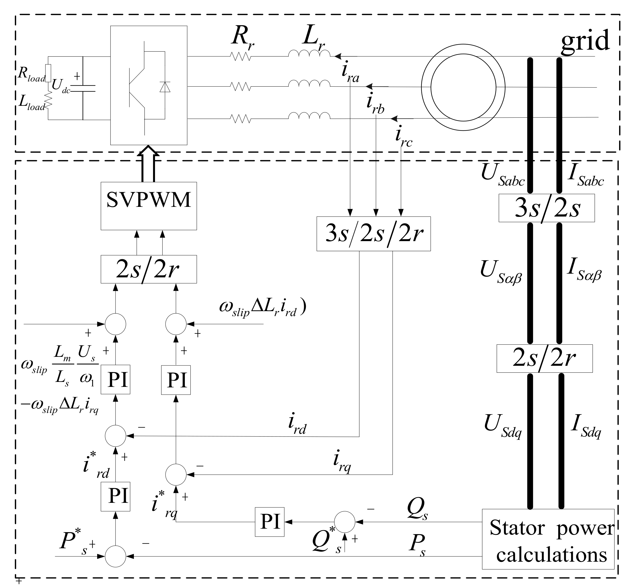
Figure 6.
The dq current inner loop control of RSC.

Figure 7.
The fitting curve of the Bessel function.

Figure 8.
The simulation process of harmonic modeling.

Figure 9.
The low-order current harmonics of GSC in sub-synchronous state.

Figure 10.
The low-order voltage harmonics of RSC in sub-synchronous state.

Figure 11.
The rotor current harmonics.

Figure 12.
The actual and calculated value of rotor harmonics: (a) voltage harmonics; (b) current harmonics.
Figure 12.
The actual and calculated value of rotor harmonics: (a) voltage harmonics; (b) current harmonics.

Figure 13.
The low-order current harmonics of RSC in super-synchronous state.

Figure 14.
The low-order current harmonics of GSC in super-synchronous state.

Figure 15.
The high-order current harmonics near 40 and 80 times the fundamental frequency.


Table 1.
The amplitude of baseband harmonics in the output voltage.
| A0n | n | A0n | |
|---|---|---|---|
| 3 | 0.095 | 11 | 0 |
| 4 | 0 | 12 | 0 |
| 5 | 0.1 | 13 | 0 |
| 6 | 0 | 14 | 0 |
| 7 | 0.0475 | 15 | 0.0235 |
| 8 | 0 | 16 | 0 |
| 9 | 0.0475 | 17 | 0.0235 |
| 10 | 0 | 18 | 0 |
Table 2.
The amplitude of baseband harmonics in the output line current.
| A0c | n | A0c | |
|---|---|---|---|
| 3 | 0 | 11 | 0 |
| 4 | 0 | 12 | 0 |
| 5 | 0.1 | 13 | 0 |
| 6 | 0 | 14 | 0 |
| 7 | 0.0475 | 15 | 0 |
| 8 | 0 | 16 | 0 |
| 9 | 0 | 17 | 0.0235 |
| 10 | 0 | 18 | 0 |
Table 3.
The difference between actual and the calculated value of voltage harmonics.
| n | A0na | A0nc | cn | cna |
|---|---|---|---|---|
| 3 | 18 | 19 | 0.5% | 5.6% |
| 5 | 21 | 20 | 0.5% | 4.8% |
| 7 | 10.5 | 9.5 | 0.5% | 9.5% |
| 9 | 12.5 | 9.5 | 1.5% | 24% |
| 15 | 6.5 | 4.7 | 0.9% | 27.7% |
| 17 | 7.8 | 4.7 | 1.55% | 39.7% |
Table 4.
The difference between actual and the calculated value of current harmonics.
| n | A0ca | A0cc | cc | cca |
|---|---|---|---|---|
| 5 | 32 | 31.5 | 0.16% | 1.6% |
| 7 | 17 | 15 | 0.63% | 11.8% |
| 17 | 11 | 7.5 | 1.11% | 31.8% |
© 2017 by the authors. Licensee MDPI, Basel, Switzerland. This article is an open access article distributed under the terms and conditions of the Creative Commons Attribution (CC BY) license (http://creativecommons.org/licenses/by/4.0/).
Share and Cite
MDPI and ACS Style
Liu, J.; Liu, Z. Harmonic Analyzing of the Double PWM Converter in DFIG Based on Mathematical Model. Energies 2017, 10, 2087. https://doi.org/10.3390/en10122087
AMA Style
Liu J, Liu Z. Harmonic Analyzing of the Double PWM Converter in DFIG Based on Mathematical Model. Energies. 2017; 10(12):2087. https://doi.org/10.3390/en10122087
Chicago/Turabian StyleLiu, Jing, and Zhigang Liu. 2017. "Harmonic Analyzing of the Double PWM Converter in DFIG Based on Mathematical Model" Energies 10, no. 12: 2087. https://doi.org/10.3390/en10122087
Note that from the first issue of 2016, this journal uses article numbers instead of page numbers. See further details here.