Flow Adjustment Inside and Around Large Finite-Size Wind Farms


Abstract
1. Introduction
2. Large-Eddy Simulations
2.1. LES Governing Equations and Modeling
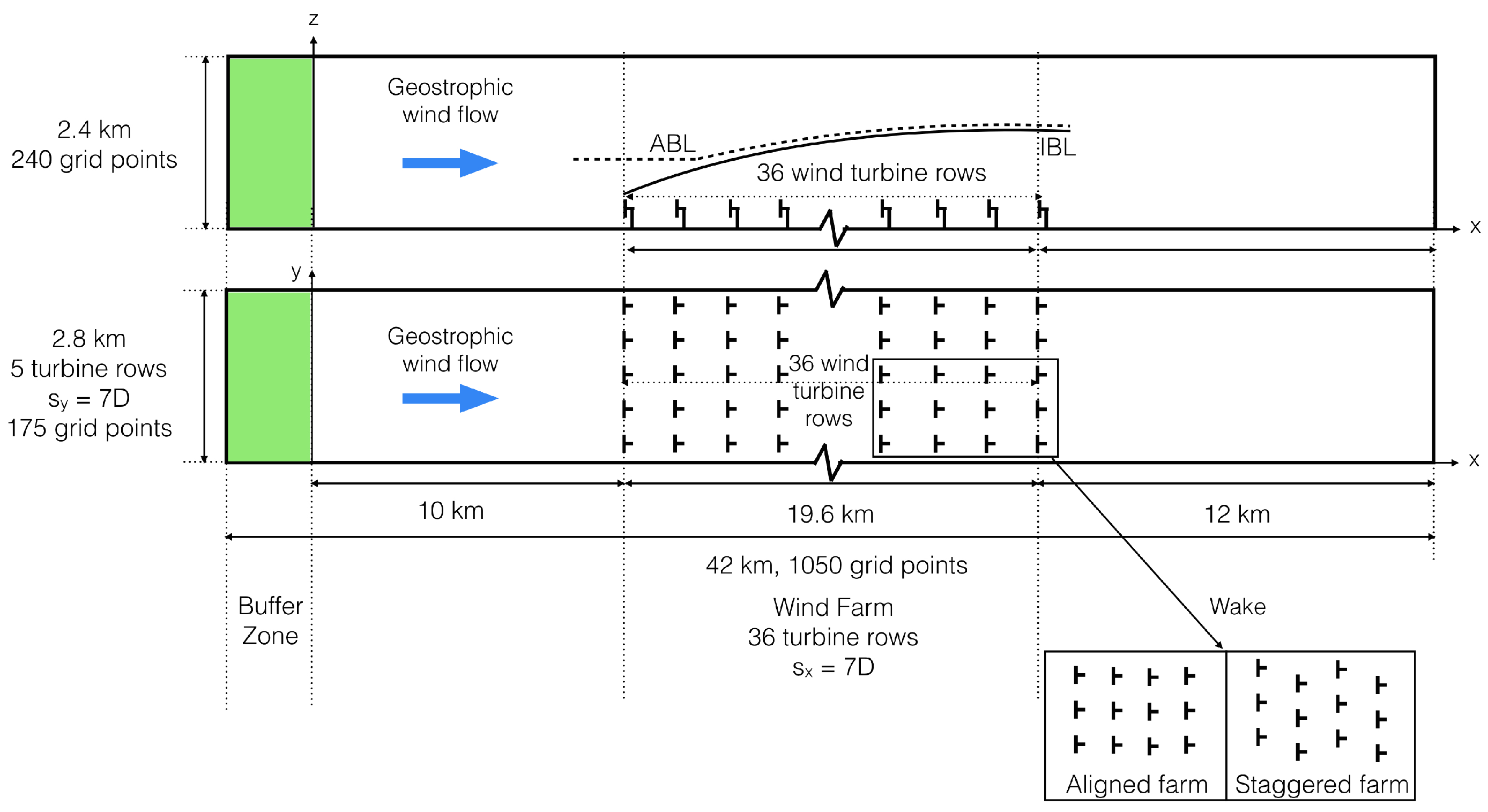
2.2. Numerical Setup
3. Suite of Simulations
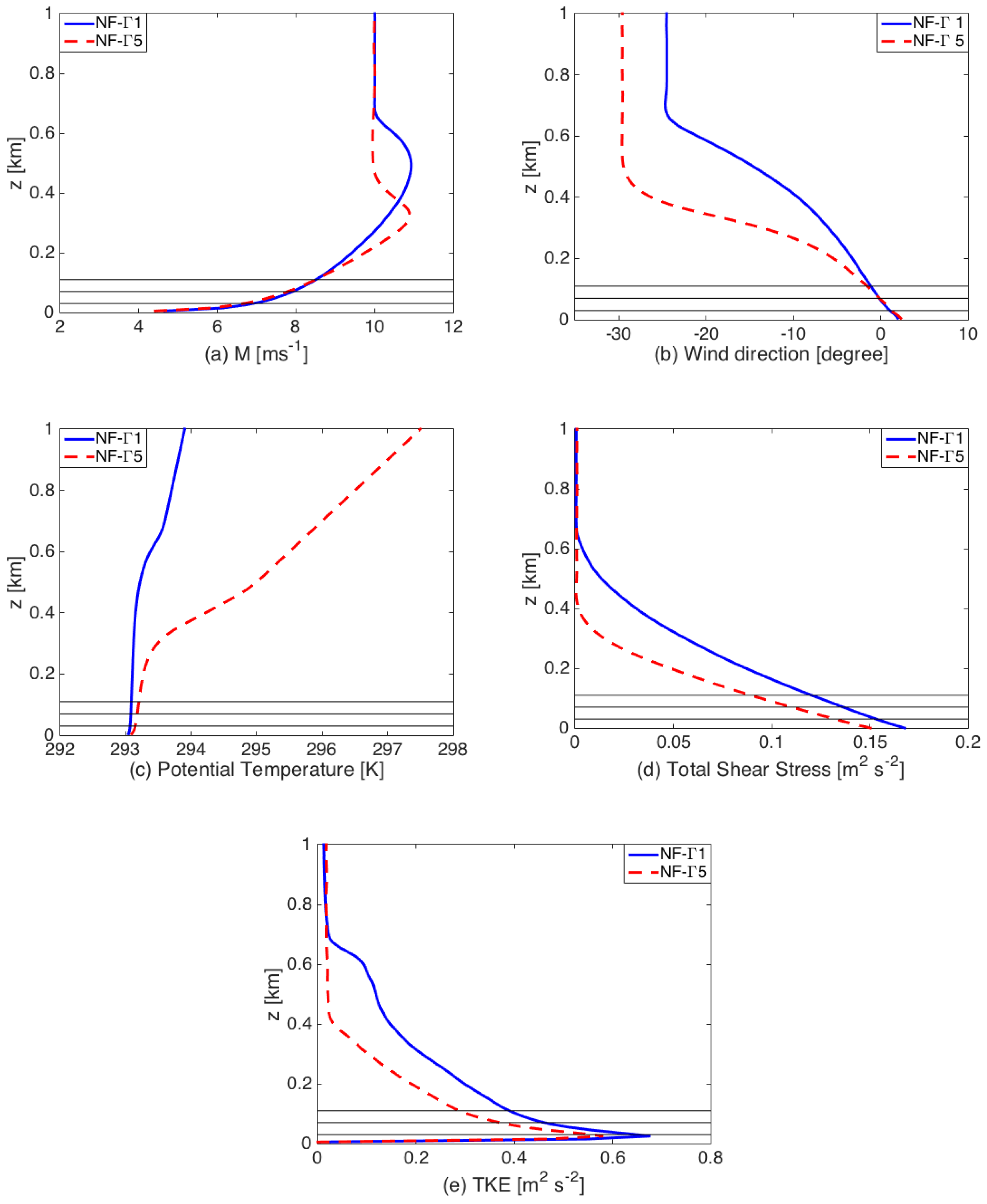
3.1. No-Farm Case
3.2. Large Finite-Size Wind Farm Simulations
3.3. Infinite Wind Farm Simulations
4. Results
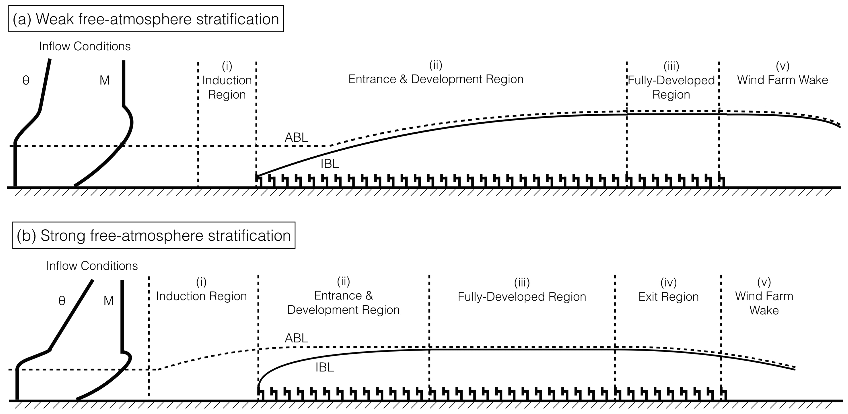
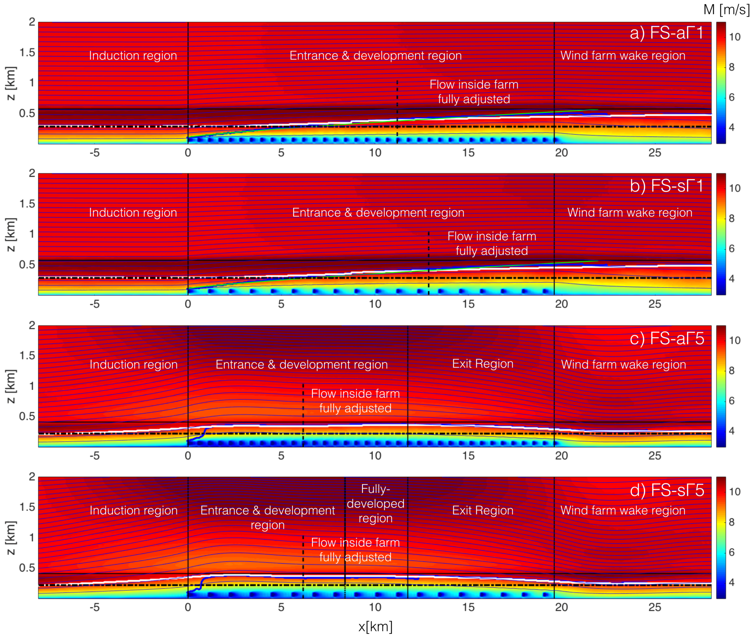
- (i)
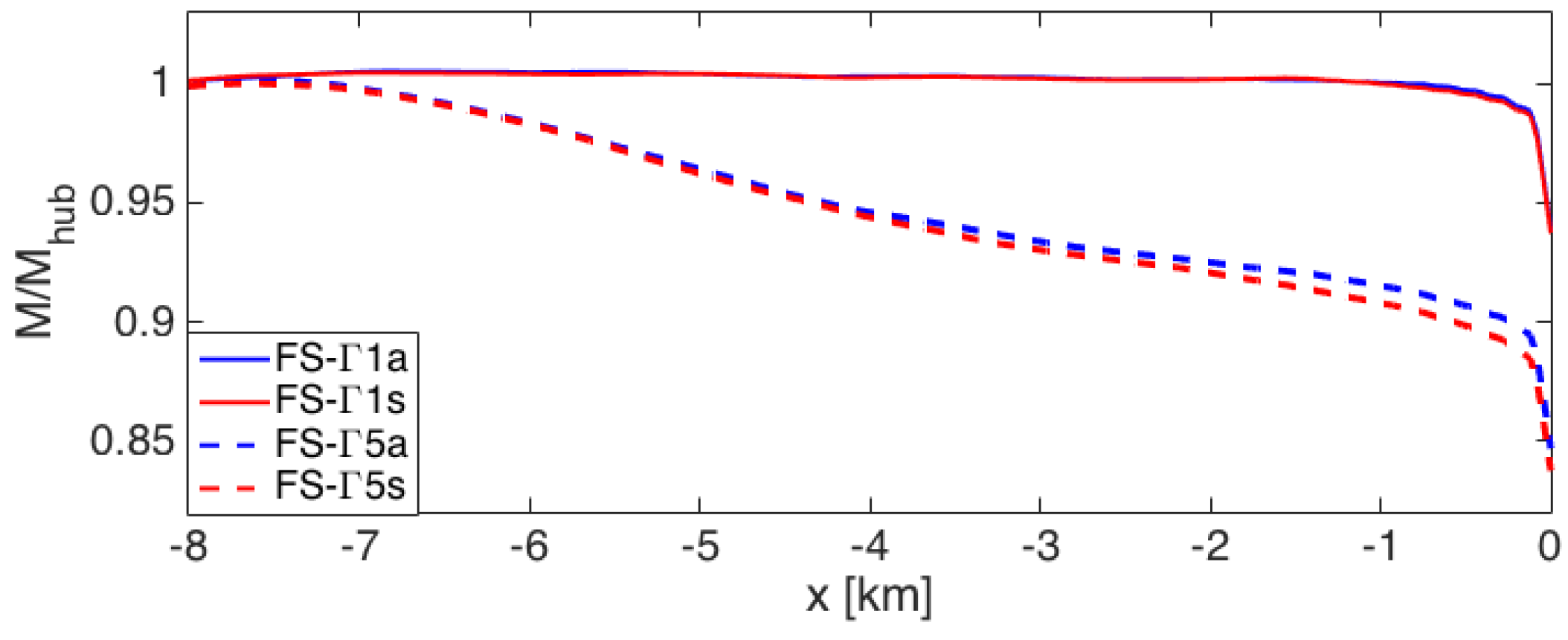
- The induction region, immediately upwind of the wind farm, where flow deceleration is induced by the wind farm due to the cumulated wind turbine blockage effect. If free-atmosphere stratification is strong enough, it could lead to a gravity-wave-induced blockage effect triggered by the farm. As a result, in that case, the velocity in this region would be significantly reduced, and the induction region could extend a few kilometers upwind of the farm.
- (ii)
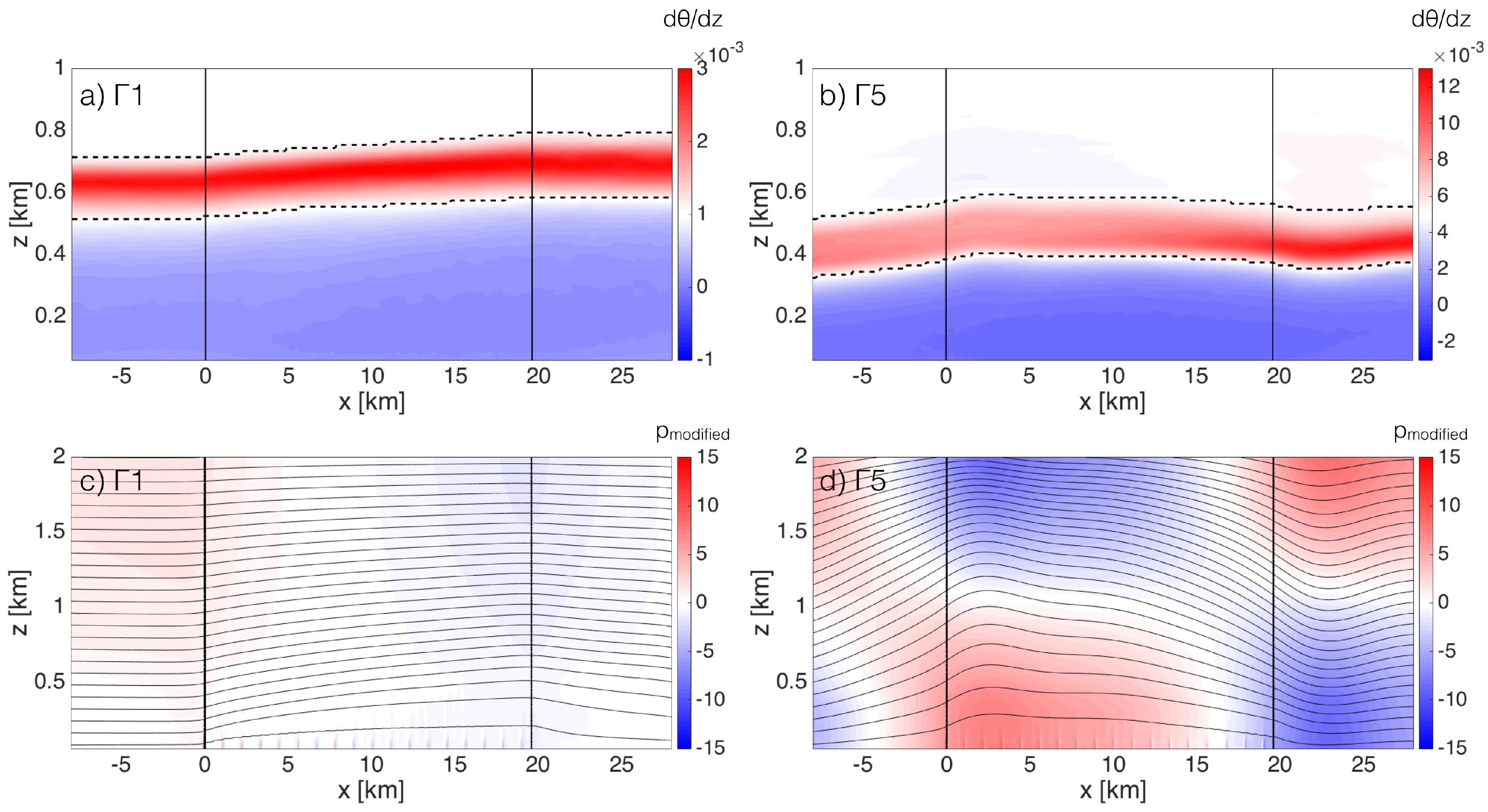
- The entrance and development region, extending immediately downwind of the leading edge of the wind farm, where the flow is decelerated because of the momentum extraction by the wind turbines. The deceleration results in an upward mass flux from the wind farm top, which slows down the flow above the farm and causes an internal boundary layer (IBL) growth. For wind farms that are large enough, the IBL could reach the ABL height and result in a modification of the ABL depth.
- (iii)
- The fully-developed region, following the entrance and development region, in which changes of flow characteristics in the streamwise direction are negligible throughout the ABL, and thus the flow is considered to be fully developed. In this region, both the IBL and ABL depths are constant and equal to the height of the infinite wind farm ABL.
- (iv)
- The exit region, upwind of the trailing edge of the wind farm, where the flow accelerates and a downward mass flux is present, resulting in a decrease in the IBL and ABL heights. If free-atmosphere stratification is strong, the downward flow could trigger upwind propagating gravity waves and an advantageous pressure gradient at the trailing farm edge. As a consequence, in that case, the favorable gravity-wave-induced pressure gradient would lead to a substantial flow acceleration in the region. The exit region could extend a few kilometers upwind of the end of the farm, similar to the length of the induction region.
- (v)
- The wind farm wake region, downwind of the wind farm trailing edge, in which the flow recovers and returns to its undisturbed inflow velocity profile.
4.1. Wind Farm Induction Region
4.2. Wind Farm Flow Entrance and Development Region
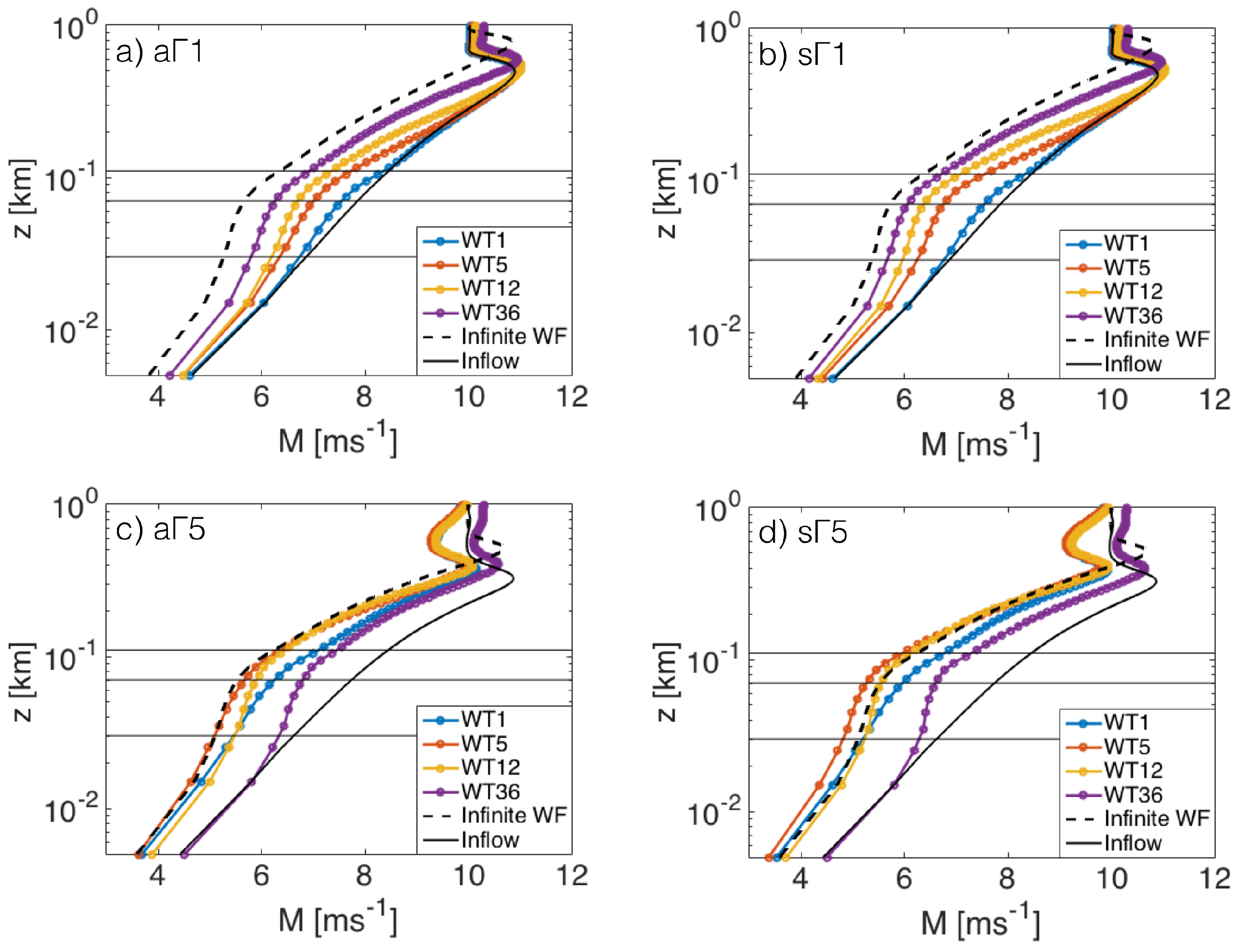
4.2.1. Velocity Adjustment
4.2.2. IBL and ABL Growth
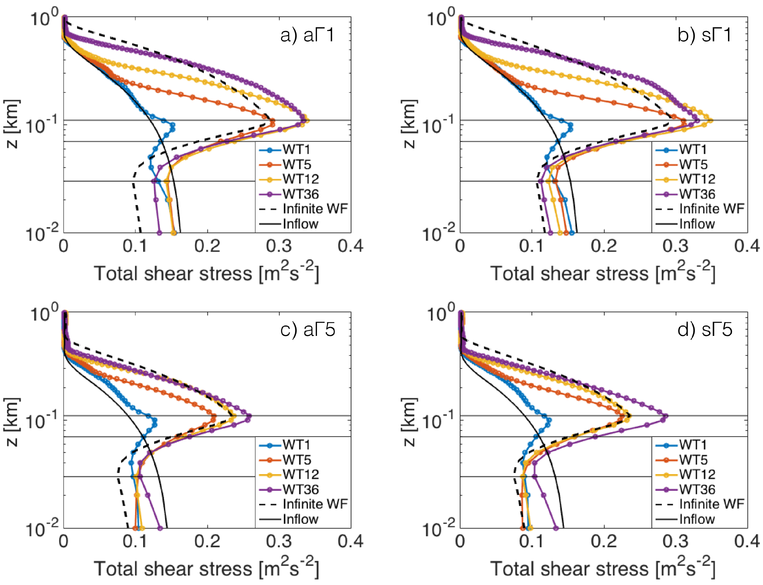
4.2.3. Turbulent Shear Stress Adjustment
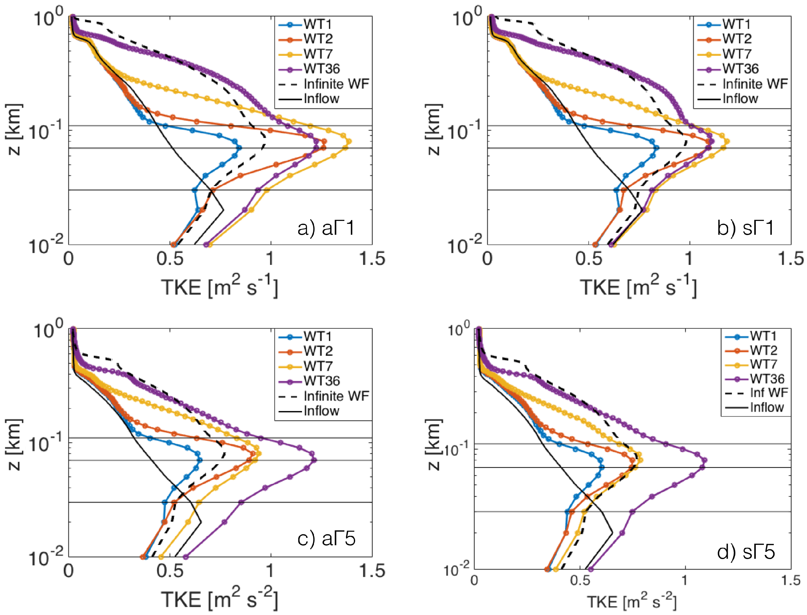
4.2.4. TKE Adjustment
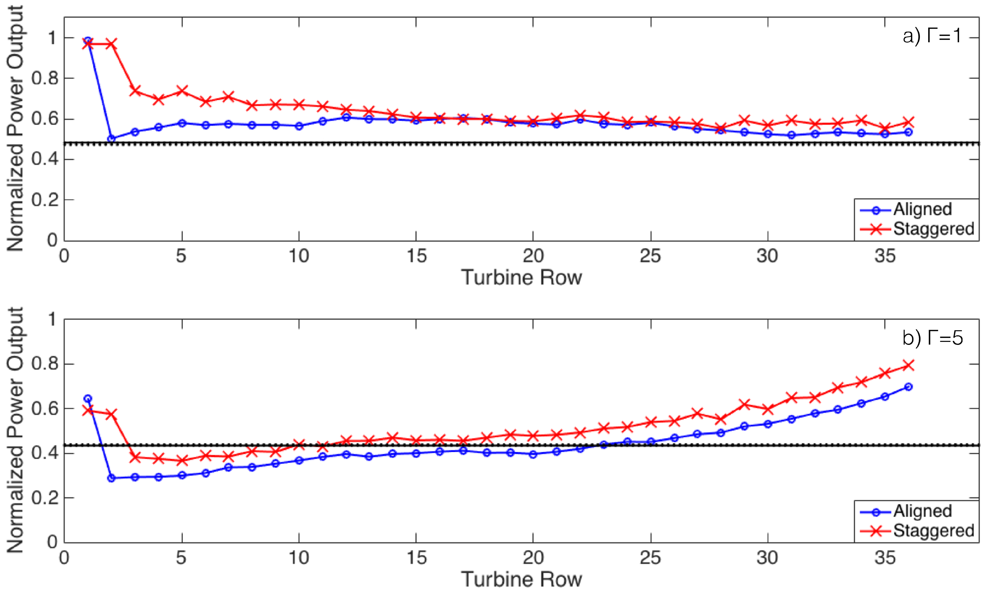
4.2.5. Wind Farm Power Output
4.3. Length of Flow Development Region
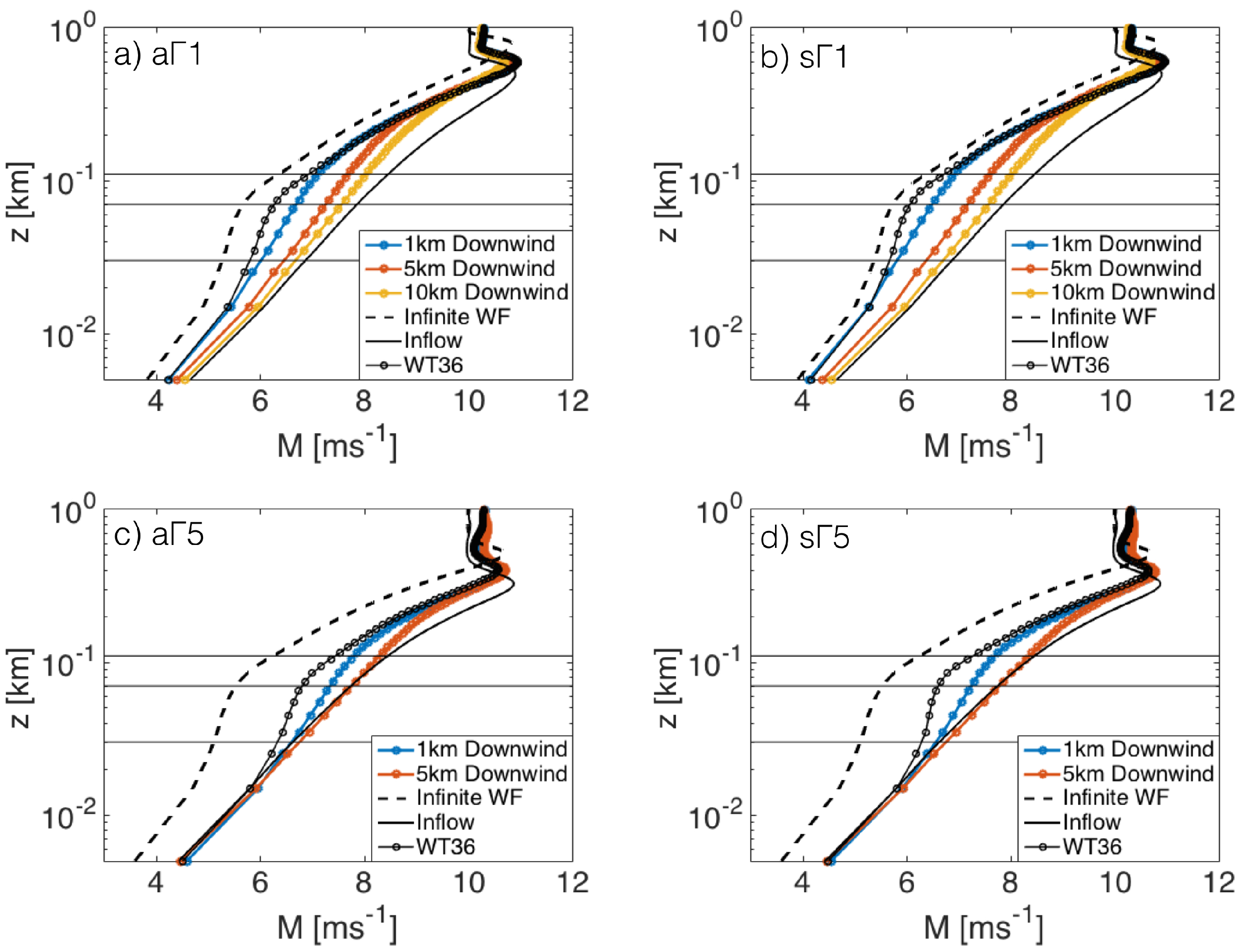
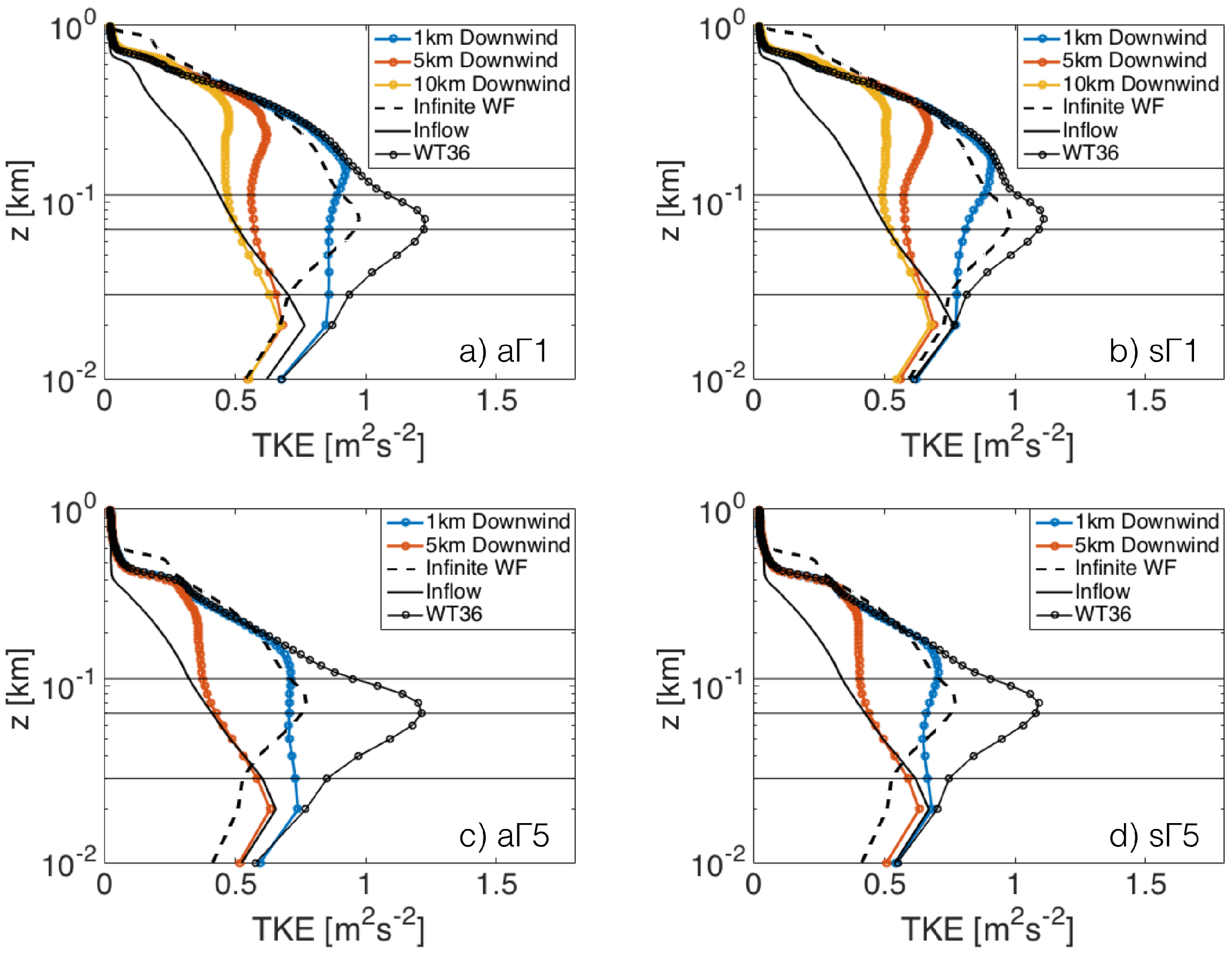
4.4. Wind Farm Wakes
5. Summary
Acknowledgments
Author Contributions
Conflicts of Interest
References
- Frandsen, S.; Barthelmie, R.; Pryor, S.; Rathmann, O.; Larsen, S.; Højstrup, J.; Thøgersen, M. Analytical modelling of wind speed deficit in large offshore wind farms. Wind Energy 2006, 9, 39–53. [Google Scholar] [CrossRef]
- Calaf, M.; Meneveau, C.; Meyers, J. Large eddy simulation study of fully developed wind-turbine array boundary layers. Phys. Fluids 2010, 22, 015110. [Google Scholar] [CrossRef]
- Meyers, J.; Meneveau, C. Large eddy simulations of large wind-turbine arrays in the atmospheric boundary layer. In Proceedings of the 48th AIAA Aerospace Sciences Meeting Including the New Horizons Forum and Aerospace Exposition, Orlando, FL, USA, 4–7 January 2010. [Google Scholar]
- Lu, H.; Porté-Agel, F. Large-eddy simulation of a very large wind farm in a stable atmospheric boundary layer. Phys. Fluids 2011, 23, 065101. [Google Scholar] [CrossRef]
- Meyers, J.; Meneveau, C. Optimal turbine spacing in fully developed wind farm boundary layers. Wind Energy 2012, 15, 305–317. [Google Scholar] [CrossRef]
- Johnstone, R.; Coleman, G.N. The turbulent Ekman boundary layer over an infinite wind-turbine array. J. Wind Eng. Ind. Aerodyn. 2012, 100, 46–57. [Google Scholar] [CrossRef]
- Abkar, M.; Porté-Agel, F. The effect of free-atmosphere stratification on boundary-layer flow and power output from very large wind farms. Energies 2013, 6, 2338–2361. [Google Scholar] [CrossRef]
- Calaf, M.; Parlange, M.B.; Meneveau, C. Large eddy simulation study of scalar transport in fully developed wind-turbine array boundary layers. Phys. Fluids 2011, 23, 126603. [Google Scholar] [CrossRef]
- VerHulst, C.; Meneveau, C. Large eddy simulation study of the kinetic energy entrainment by energetic turbulent flow structures in large wind farms. Phys. Fluids 2014, 26, 025113. [Google Scholar] [CrossRef]
- Abkar, M.; Porté-Agel, F. Mean and turbulent kinetic energy budgets inside and above very large wind farms under conventionally-neutral condition. Renew. Energy 2014, 70, 142–152. [Google Scholar] [CrossRef]
- Porté-Agel, F.; Wu, Y.T.; Lu, H.; Conzemius, R. Large-eddy simulation of atmospheric boundary layer flow through wind turbines and wind farms. J. Wind Eng. Ind. Aerodyn. 2011, 99, 154–168. [Google Scholar] [CrossRef]
- Porté-Agel, F.; Wu, Y.T.; Chen, C.H. A numerical study of the effects of wind direction on turbine wakes and power losses in a large wind farm. Energies 2013, 6, 5297–5313. [Google Scholar] [CrossRef]
- Wu, Y.T.; Porté-Agel, F. Simulation of turbulent flow inside and above wind farms: Model validation and layout effects. Bound.-Layer Meteorol. 2013, 146, 181–205. [Google Scholar] [CrossRef]
- Wu, Y.T.; Porté-Agel, F. Modeling turbine wakes and power losses within a wind farm using LES: An application to the Horns Rev offshore wind farm. Renew. Energy 2015, 75, 945–955. [Google Scholar] [CrossRef]
- Allaerts, D.; Meyers, J. Effect of inversion-layer height and Coriolis forces on developing wind-farm boundary layers. In Proceedings of the 34th Wind Energy Symposium, San Diego, CA, USA, 4–8 January 2016; p. 1989. [Google Scholar]
- Ivanell, S. Numerical Computations of Wind Turbine Wakes. Ph.D. Thesis, Gotland University, Visby, Sweden, 2009. [Google Scholar]
- Churchfield, M.J.; Lee, S.; Moriarty, P.J.; Martinez, L.A.; Leonardi, S.; Vijayakumar, G.; Brasseur, J.G. A large-eddy simulation of wind-plant aerodynamics. In Proceedings of the 50th AIAA Aerospace Sciences Meeting Including the New Horizons Forum and Aerospace Exposition, Aerospace Sciences Meetings, Nashville, TN, USA, 9–12 January 2012. [Google Scholar]
- Eriksson, O.; Lindvall, J.; Breton, S.P.; Ivanell, S. Wake downstream of the Lillgrund wind farm-A Comparison between LES using the actuator disc method and a Wind farm Parametrization in WRF. J. Phys. Conf. Ser. 2015, 625, 012028. [Google Scholar] [CrossRef]
- Nilsson, K.; Ivanell, S.; Hansen, K.; Mikkelsen, R.; Sørensen, J.; Breton, S.P.; Henningson, D. Large-eddy simulations of the Lillgrund wind farm. Wind Energy 2015, 18, 449–467. [Google Scholar] [CrossRef]
- Abkar, M.; Sharifi, A.; Porté-Agel, F. Wake flow in a wind farm during a diurnal cycle. J. Turbul. 2016, 17, 420–441. [Google Scholar] [CrossRef]
- Allaerts, D.; Meyers, J. Boundary-layer development and gravity waves in conventionally neutral wind farms. J. Fluid Mech. 2017, 814, 95–130. [Google Scholar] [CrossRef]
- Barthelmie, R.; Hansen, K.; Frandsen, S.; Rathmann, O.; Schepers, J.; Schlez, W.; Phillips, J.; Rados, K.; Zervos, A.; Politis, E.; et al. Modelling and measuring flow and wind turbine wakes in large wind farms offshore. Wind Energy 2009, 12, 431–444. [Google Scholar] [CrossRef]
- Creech, A.; Früh, W.G.; Maguire, A.E. Simulations of an offshore wind farm using large-eddy simulation and a torque-controlled actuator disc model. Surv. Geophys. 2015, 36, 427–481. [Google Scholar] [CrossRef]
- Ghaisas, N.S.; Archer, C.L.; Xie, S.; Wu, S.; Maguire, E. Evaluation of layout and atmospheric stability effects in wind farms using large-eddy simulation. Wind Energy 2017, 20, 1227–1240. [Google Scholar] [CrossRef]
- Barthelmie, R.; Pryor, S.; Frandsen, S.; Hansen, K.; Schepers, J.; Rados, K.; Schlez, W.; Neubert, A.; Jensen, L.; Neckelmann, S. Quantifying the impact of wind turbine wakes on power output at offshore wind farms. J. Atmos. Ocean. Technol. 2010, 27, 1302–1317. [Google Scholar] [CrossRef]
- Zilitinkevich, S.; Baklanov, A.; Rost, J.; Smedman, A.S.; Lykosov, V.; Calanca, P. Diagnostic and prognostic equations for the depth of the stably stratified Ekman boundary layer. Q. J. R. Meteorol. Soc. 2002, 128, 25–46. [Google Scholar] [CrossRef]
- Nygaard, N.G. Wakes in very large wind farms and the effect of neighbouring wind farms. J. Phys. Conf. Ser. 2014, 524, 012162. [Google Scholar] [CrossRef]
- Jensen, N.O. A Note on Wind Generator Interaction; Risø National Laboratory: Roskilde, Denmark, 1983. [Google Scholar]
- Bleeg, J.; Traiger, E.; Purcell, M.; Landberg, L. Wind farm blockage and its impact on energy production. In Proceedings of the Wind Energy Science Conference 2017, Lyngby, Denmark, 26–29 June 2017. [Google Scholar]
- Porté-Agel, F.; Meneveau, C.; Parlange, M. A scale-dependent dynamic model for large-eddy simulation: Application to a neutral atmospheric boundary layer. J. Fluid Mech. 2000, 415, 261–284. [Google Scholar] [CrossRef]
- Porté-Agel, F. A scale-dependent dynamic model for scalar transport in large-eddy simulations of the atmospheric boundary layer. Bound.-Layer Meteorol. 2004, 112, 81–105. [Google Scholar] [CrossRef]
- Stoll, R.; Porté-Agel, F. Dynamic subgrid-scale models for momentum and scalar fluxes in large-eddy simulations of neutrally stratified atmospheric boundary layers over heterogeneous terrain. Water Resour. Res. 2006, 42. [Google Scholar] [CrossRef]
- Wu, Y.T.; Porté-Agel, F. Large-eddy simulation of wind-turbine wakes: Evaluation of turbine parametrisations. Bound.-Layer Meteorol. 2011, 138, 345–366. [Google Scholar] [CrossRef]
- Albertson, J.; Parlange, M. Surface length scales and shear stress: Implications for land-atmosphere interaction over complex terrain. Water Resour. Res. 1999, 35, 2121–2132. [Google Scholar] [CrossRef]
- Orszag, S. Transform method for the calculation of vector-coupled sums: Application to the spectral form of the vorticity equation. J. Atmos. Sci. 1970, 27, 890–895. [Google Scholar] [CrossRef]
- Canuto, C.; Hussaini, M.Y.; Quarteroni, A.M.; Thomas, A., Jr. Spectral Methods in Fluid Dynamics; Springer Science & Business Media: Berlin, Germany, 2012. [Google Scholar]
- Stoll, R.; Porté-Agel, F. Surface heterogeneity effects on regional-scale fluxes in stable boundary layers: Surface temperature transitions. J. Atmos. Sci. 2009, 66, 412–431. [Google Scholar] [CrossRef]
- Moeng, C.H. A large-eddy-simulation model for the study of planetary boundary-layer turbulence. J. Atmos. Sci. 1984, 41, 2052–2062. [Google Scholar] [CrossRef]
- Abkar, M.; Porté-Agel, F. A new boundary condition for large-eddy simulation of boundary-layer flow over surface roughness transitions. J. Turbul. 2012, 13. [Google Scholar] [CrossRef]
- Hansen, K.S.; Barthelmie, R.J.; Jensen, L.E.; Sommer, A. The impact of turbulence intensity and atmospheric stability on power deficits due to wind turbine wakes at Horns Rev wind farm. Wind Energy 2012, 15, 183–196. [Google Scholar] [CrossRef]
- Munters, W.; Meneveau, C.; Meyers, J. Turbulent inflow precursor method with time-varying direction for large-eddy simulations and applications to wind farms. Bound.-Layer Meteorol. 2016, 159, 305–328. [Google Scholar] [CrossRef]
- Sescu, A.; Meneveau, C. A control algorithm for statistically stationary large-eddy simulations of thermally stratified boundary layers. Q. J. R. Meteorol. Soc. 2014, 140, 2017–2022. [Google Scholar] [CrossRef]
- Belcher, S.; Jerram, N.; Hunt, J. Adjustment of a turbulent boundary layer to a canopy of roughness elements. J. Fluid Mech. 2003, 488, 369–398. [Google Scholar] [CrossRef]
- Medici, D.; Ivanell, S.; Dahlberg, J.Å.; Alfredsson, P.H. The upstream flow of a wind turbine: Blockage effect. Wind Energy 2011, 14, 691–697. [Google Scholar] [CrossRef]
- Simley, E.; Angelou, N.; Mikkelsen, T.; Sjöholm, M.; Mann, J.; Pao, L.Y. Characterization of wind velocities in the upstream induction zone of a wind turbine using scanning continuous-wave lidars. J. Renew. Sustain. Energy 2016, 8, 013301. [Google Scholar] [CrossRef]
- Branlard, E. Wind Turbine Aerodynamics and Vorticity-Based Methods: Fundamentals and Recent Applications; Springer: Berlin, Germany, 2017; Volume 7. [Google Scholar]
- Queney, P. The problem of air flow over mountains: A summary of theoretical studies. Bull. Am. Meteorol. Soc. 1948, 29, 16–26. [Google Scholar]
- Durran, D.R. Mountain waves and downslope winds. In Atmospheric Processes Over Complex Terrain; Springer: Berlin, Germany, 1990; pp. 59–81. [Google Scholar]
- Smith, R.B. Gravity wave effects on wind farm efficiency. Wind Energy 2010, 13, 449–458. [Google Scholar] [CrossRef]
- Reinecke, P.A.; Durran, D.R. Estimating topographic blocking using a Froude number when the static stability is nonuniform. J. Atmos. Sci. 2008, 65, 1035–1048. [Google Scholar] [CrossRef]
- Vosper, S.; Wells, H.; Brown, A. Accounting for non-uniform static stability in orographic drag parametrization. Q. J. R. Meteorol. Soc. 2009, 135, 815–822. [Google Scholar] [CrossRef]
- Rominger, J.T.; Nepf, H.M. Flow adjustment and interior flow associated with a rectangular porous obstruction. J. Fluid Mech. 2011, 680, 636–659. [Google Scholar] [CrossRef]
- Claussen, M. The flow in a turbulent boundary layer upstream of a change in surface roughness. Bound.-Layer Meteorol. 1987, 40, 31–86. [Google Scholar] [CrossRef]
- Belcher, S.E.; Harman, I.N.; Finnigan, J.J. The wind in the willows: Flows in forest canopies in complex terrain. Annu. Rev. Fluid Mech. 2012, 44, 479–504. [Google Scholar] [CrossRef]
- Garratt, J. The internal boundary layer—A review. Bound.-Layer Meteorol. 1990, 50, 171–203. [Google Scholar] [CrossRef]
- Elliott, W.P. The growth of the atmospheric internal boundary layer. Trans. Am. Geophys. Union 1958, 39, 1048–1054. [Google Scholar] [CrossRef]
- Morse, A.; Gardiner, B.; Marshall, B. Mechanisms controlling turbulence development across a forest edge. Bound.-Layer Meteorol. 2002, 103, 227–251. [Google Scholar] [CrossRef]
- Shir, C. A numerical computation of air flow over a sudden change of surface roughness. J. Atmos. Sci. 1972, 29, 304–310. [Google Scholar] [CrossRef]
- Stevens, R.J.; Gayme, D.F.; Meneveau, C. Large eddy simulation studies of the effects of alignment and wind farm length. J. Renew. Sustain. Energy 2014, 6, 023105. [Google Scholar] [CrossRef]
- Porté-Agel, F.; Lu, H.; Wu, Y.T. Interaction between large wind farms and the atmospheric boundary layer. Procedia IUTAM 2014, 10, 307–318. [Google Scholar] [CrossRef]
- Markfort, C.D.; Zhang, W.; Porté-Agel, F. Turbulent flow and scalar transport through and over aligned and staggered wind farms. J. Turbul. 2012, 13, N33. [Google Scholar] [CrossRef]
- Frandsen, S.T.; Jørgensen, H.E.; Barthelmie, R.; Rathmann, O.; Badger, J.; Hansen, K.; Ott, S.; Rethore, P.E.; Larsen, S.E.; Jensen, L.E. The making of a second-generation wind farm efficiency model complex. Wind Energy 2009, 12, 445–458. [Google Scholar] [CrossRef]


| Case | (K/km) | Number of Turbines | Turbine Arrangement | (km3) | ||
|---|---|---|---|---|---|---|
| No-Farm Case | ||||||
| NF | 1 | - | - | - | ||
| NF | 5 | - | - | - | ||
| Large Finite-Size Wind Farm Case | ||||||
| FS−s | 1 | Staggered | ||||
| FS−a | 1 | Aligned | ||||
| FS−s | 5 | Staggered | ||||
| FS−a | 5 | Aligned | ||||
| Infinite Wind Farm Case | ||||||
| Inf−s | 1 | Staggered | ||||
| Inf−a | 1 | Aligned | ||||
| Inf−s | 5 | Staggered | ||||
| Inf−a | 5 | Aligned | ||||
| (K/km) | (m·s) | (m) | N (s | (m) | (K) | |
|---|---|---|---|---|---|---|
| 9.63 | 710 | 0.0057 | 2370 | 295 | 0.94 | |
| 8.05 | 510 | 0.013 | 1220 | 299 | 1.31 |
© 2017 by the authors. Licensee MDPI, Basel, Switzerland. This article is an open access article distributed under the terms and conditions of the Creative Commons Attribution (CC BY) license (http://creativecommons.org/licenses/by/4.0/).
Share and Cite
Wu, K.L.; Porté-Agel, F. Flow Adjustment Inside and Around Large Finite-Size Wind Farms. Energies 2017, 10, 2164. https://doi.org/10.3390/en10122164
Wu KL, Porté-Agel F. Flow Adjustment Inside and Around Large Finite-Size Wind Farms. Energies. 2017; 10(12):2164. https://doi.org/10.3390/en10122164
Chicago/Turabian StyleWu, Ka Ling, and Fernando Porté-Agel. 2017. "Flow Adjustment Inside and Around Large Finite-Size Wind Farms" Energies 10, no. 12: 2164. https://doi.org/10.3390/en10122164
APA StyleWu, K. L., & Porté-Agel, F. (2017). Flow Adjustment Inside and Around Large Finite-Size Wind Farms. Energies, 10(12), 2164. https://doi.org/10.3390/en10122164