k-Nearest Neighbor Neural Network Models for Very Short-Term Global Solar Irradiance Forecasting Based on Meteorological Data

Abstract
:1. Introduction
2. Modelling and Data Description
3. k-Nearest Neighbor and Artificial Neural Network Model for Forecasting Global Solar Irradiance Based on Meteorological Data
3.1. k-Nearest-Neighbors
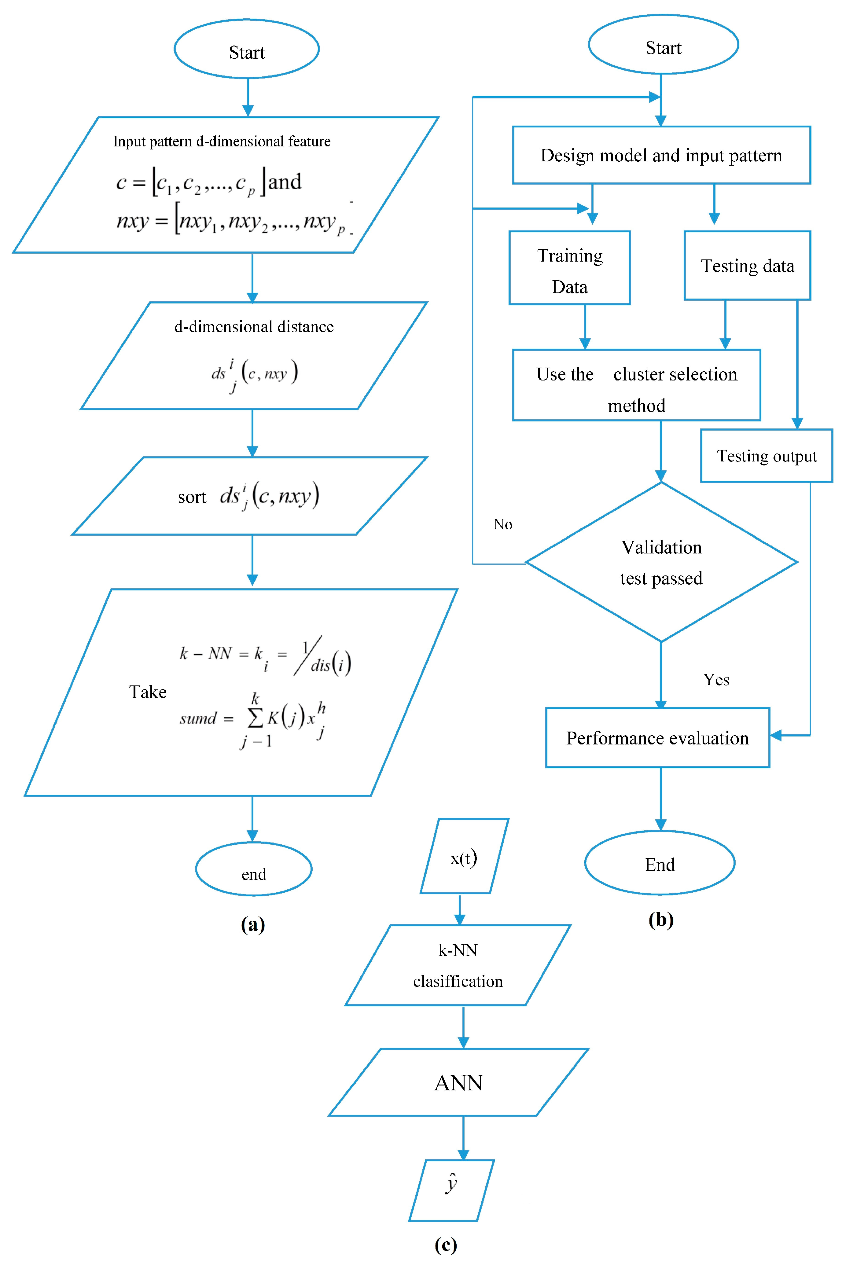
k-Nearest Neighbor Modelling
- (1)
- The matrix scenarios composed modelling stage which includes form d-dimensional feature vectors C or nxy from the historical data x: and or x: ; Their corresponding successors are denoted as xh. They are given two pieces point c and nxy in a space vector of n-dimensional c (c1, c2, ..., cn) and nxy (nxy1, nxy2, ..., nxyn).
- (2)
- The distance calculate vector stage which includes form n-dimensional distance vector = Di for each testing vector C or nxy by calculating the Euclidean distance between = Di and the remaining:where Di is the value of the dependent variable historical data set and Dj is the value of the dependent the nearest neighbor based on distance:where is value of the dependent variable GSI, is the position coordinat PV station (magnitude of nearest neighbors) is the d-dimensional feature vectors, The index j is the current condition, i is the historical dataset, k = K the number of elements in the nearest neighbors, q is the historical dataset and where x, y are scenarios composed of k features and p is the number of the k-NN based on their distance from the current condition (j) in which the nearest have the lowest order (p = 1, ..., k).
- (3)
- Select the value distance of the k-NN stage, which includes the sort in ascending order and select the first K entries as the nearest neighbors Dk, k ∈ {1, ..., K}.
- (4)
- Select the best value of k used in modelling the k-NN stage, because a high k value will reduce the effect of noise on the classification, but it will make the boundaries between each classification becomes increasingly blurred. Form a kernel function:where K(j) = ki is the value k-NN (kernel function), i is the historical data set and the index j is the number of the k-NN based on their distance from the current condition (i) in which the nearest have the lowest order (j = 1, ..., K), and K is the length data sets, and the distance between the current and previous condition [25].
- (5)
- Calculate the final estimation stage, using Equation (5):where is the magnitude of nearest neighbor j, j is the order of the nearest neighbors based on their distance from the current condition (h) in which the nearest have the lowest order (j = 1, ..., k), sumd is the karnel function, k is the length of data sets, and Kj is the kernel function.
3.2. Artificial Neural Network
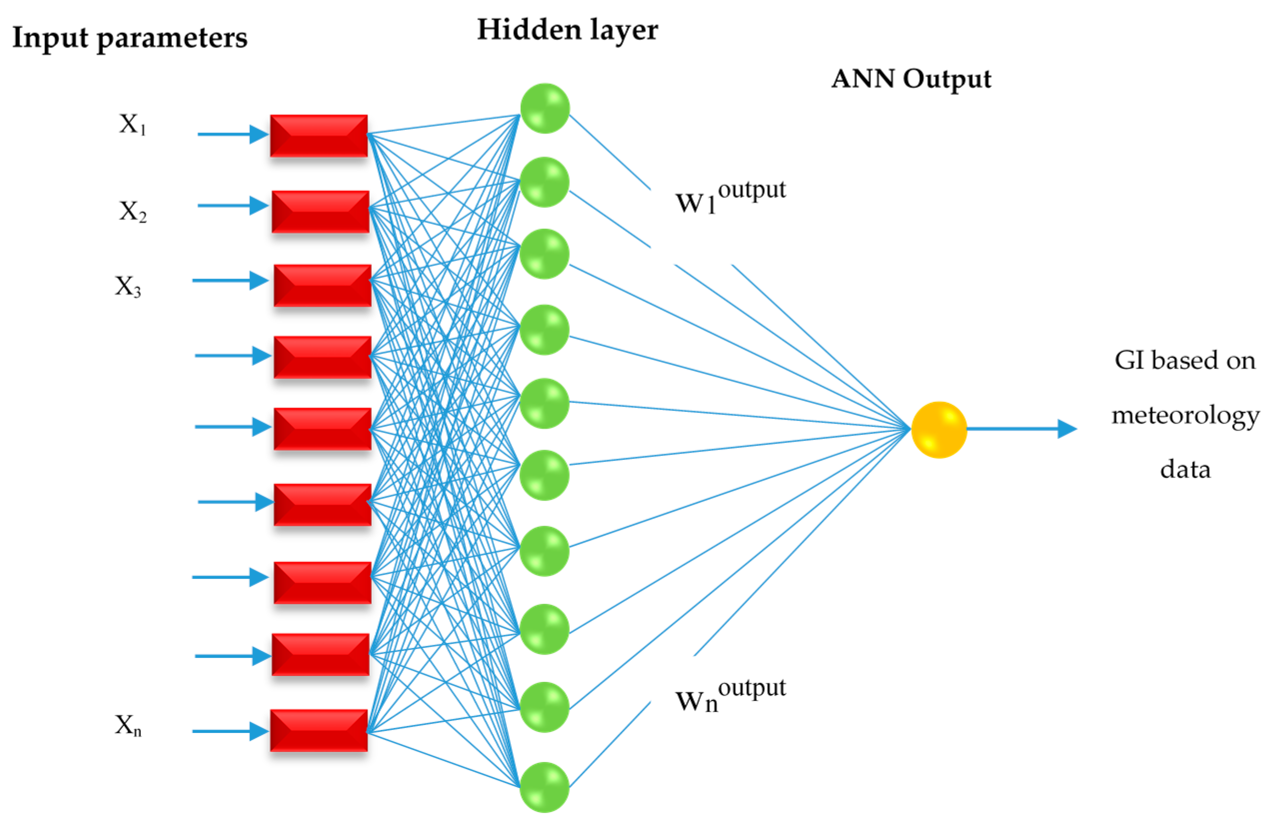
Artificial Neural Network Modelling
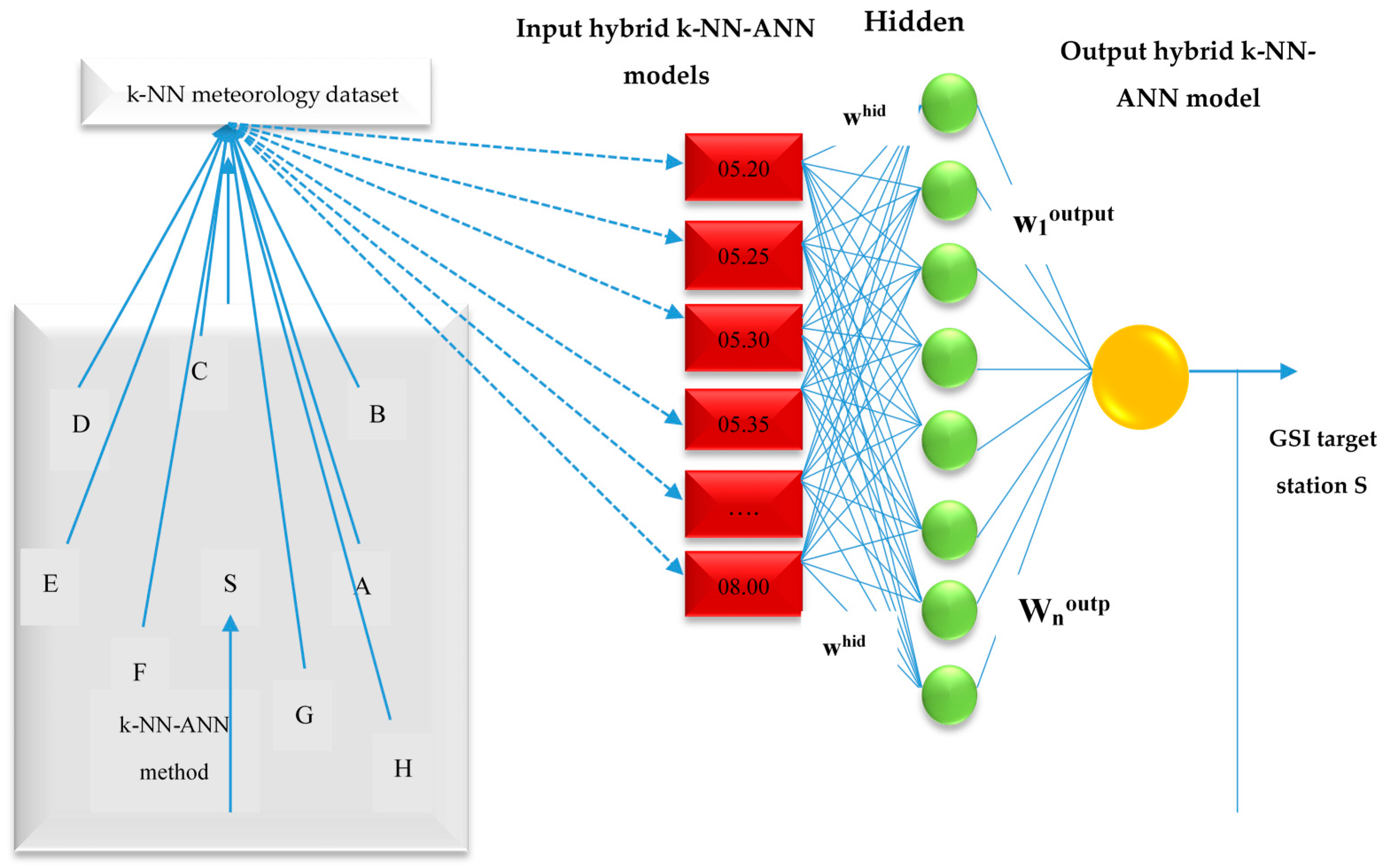
3.3. k-Nearest Neighbor and Artificial Neural Network Modelling
- Step 1:
- Calculate the distance of each data parameter:and the weight distance is:where is the Euclidan distance GSI
- is the Euclidan distance temperature
- is the Euclidan distance humidity
- is the Euclidan distance wind speed
- is the Euclidan distance wind direct
- is the weight distance at GSI
- is the weight distance at temperature
- is the weight distance at humidity
- is the weight distance at wind speed
- is the weight distance at wind direct
- GI is the global irradiance
- Ta is the temperature
- Ho is the humidity
- Ws is the wind speed
- Wd is the wind direct
- is the d dimensional feature vectors GSI
- is the d dimensional feature vectors temperature
- is the d dimensional feature vectors humidity
- is the d dimensional feature vectors wind speed
- is the d dimensional feature vectors wind direct
- is the position coordinat PV station (magnitude of nearest neighbors)
- is the d-dimensional feature vectors
- sumd is the kernel function:
- i is the historical data set
- j is the current condition, i is the historical dataset, k = K the number of elements in the nearest neighbors
- q is the historical dataset and where x, y are scenarios composed of k features and p is the number of the k-NN based on their distance from the current condition (j) in which the nearest have the lowest order (p = 1, ..., k).
- Step 2:
- Calculate number of nearest neighbors:where k is the distance nearest neighbor, i is the historical dataset and n is the total number of features (i = 1, 2, ..., n)
- Step 3:
- Calculate the final estimation as:where is the value magnitude of the k-NN j, j is the order of the nearest neighbors based on distance (h) in which the nearest have the lowest order (j = 1, ..., k), sumd is the karnel function, k is the length of data sets, and the distance between the current and previous condition and Kj is the kernel function.
- Step 4:
- Training data and testing data using ANN method are obtained from the following steps:
- The final estimation of GSI from k-NN method is into training sets, validation sets, and test sets for ANN model.
- Architecture model and training sets parameters (create and configure the neural network, initialize the weights layer and biases layer) are selected
- Model GSI forecast using the training set are run
- Model forecasting is validated using the validation set
- Step b–e are repeated using different architectures model forecasting and training set parameters
- The optimum model is chosen and inserted into training process using data from the training set and validation set
- The ultimate forecasting model is assessed using the test set
- Step 5:
- Perform predictions for future GSI data at the Station S with k-NN-ANN
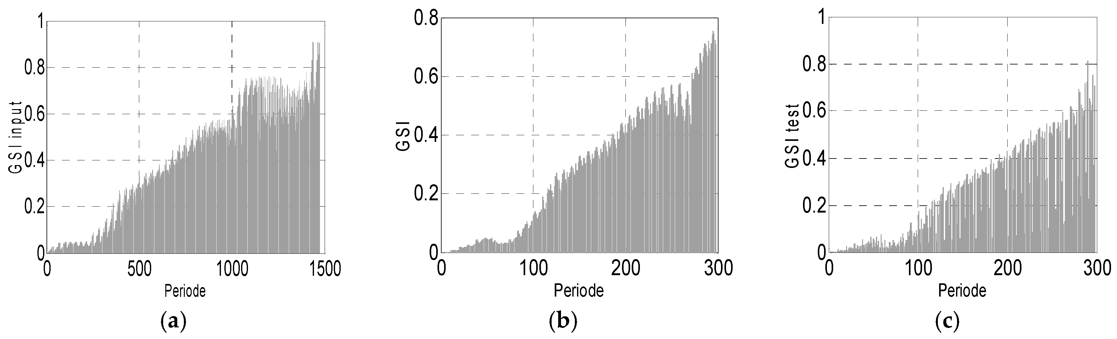
3.4. Normalization
4. Results and Discussion
Data
- (a)
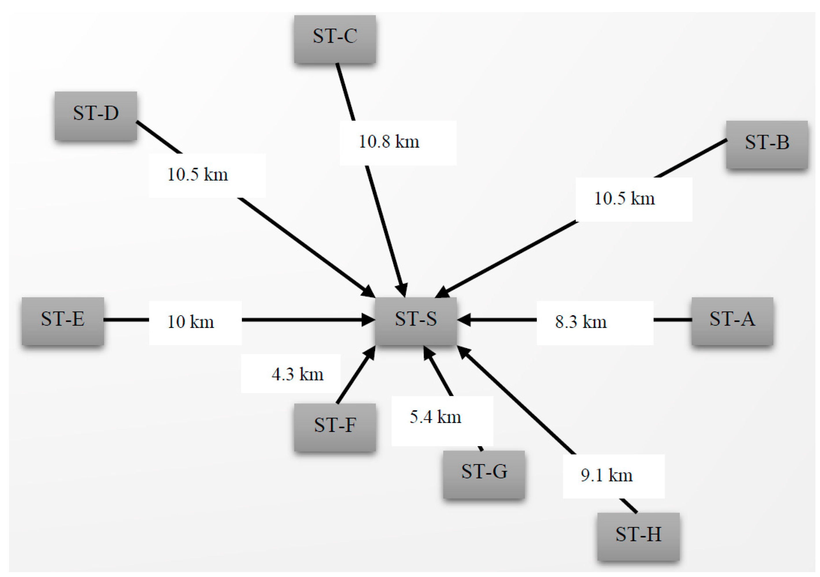
- The first stage is calculating d-dimensional feature and n-dimensional distance based on the Euclidean (k-NN model) every hour for all of the PV stations. Data shown in Table 1 are the order parameters of each PV station, i.e., angle, distance and position coordinates. The table summarizes all possible combinations of variables to be considered as an input for k-NN method.
- (b)
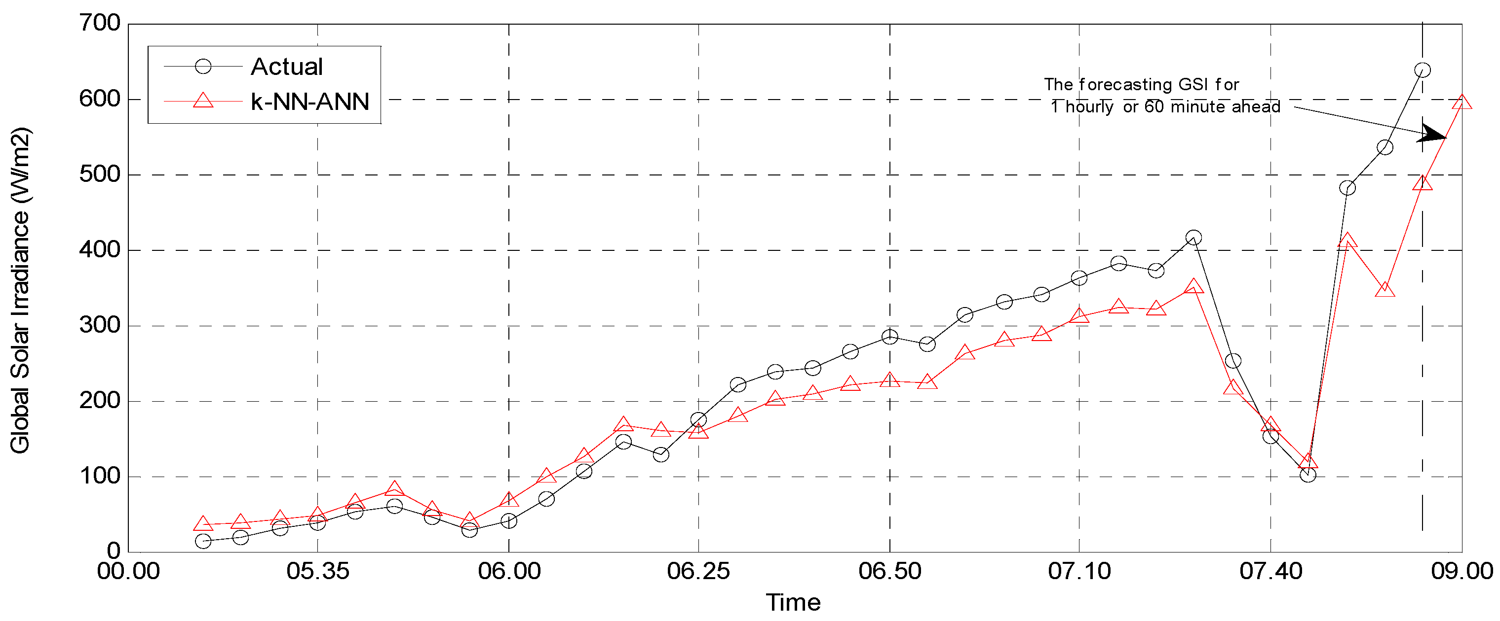
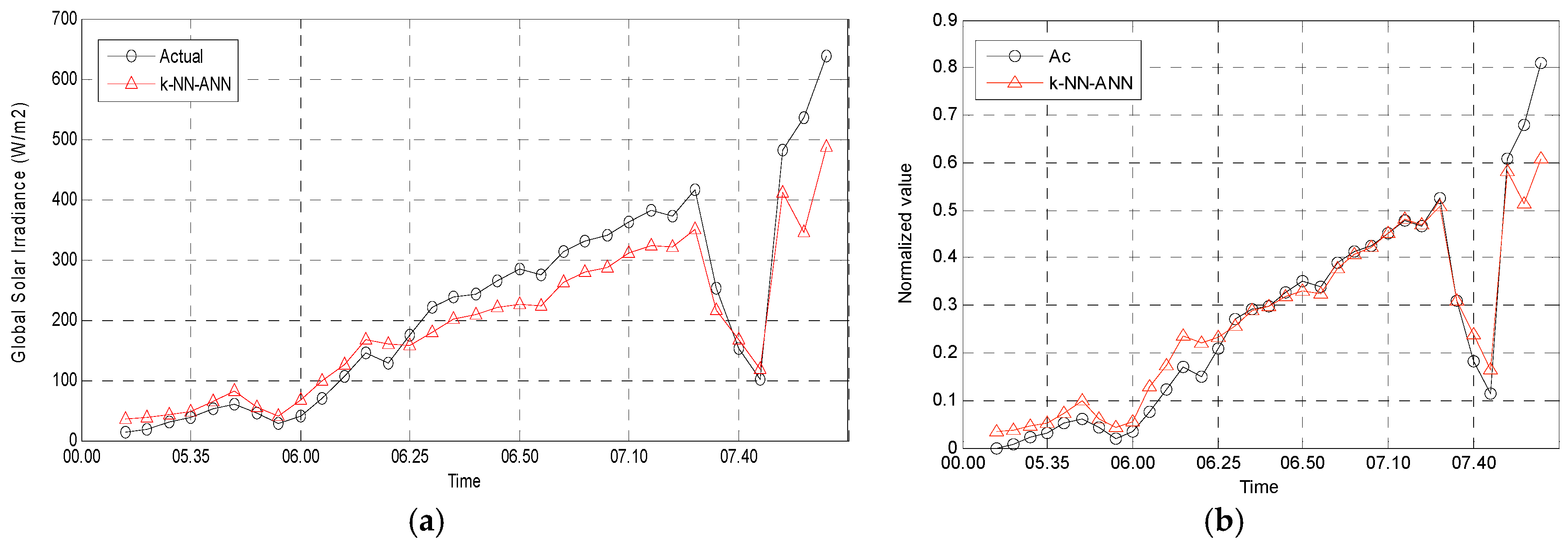
- The second stage uses the ANN based on the assumption that the existing data input is a combination of the results obtained from the k-NN model. The research model proposed in this study seeks to estimate and predict a PV station production 60 min ahead, which position is located at the center and surrounded by eight other PV stations.
5. Conclusions
- A different formulation for very short term GSI forecasting using k-NN-ANN modelling based on meteorology data is proposed. The proposed model attempting to shape the patterns of a polynomial equation shows that the proposed model forecasting is more better. The variable meteorology data weather is of great very importance and affects the resulting GSI forecasting output.
- The new model proposed in this study is a combination of k-NN modelling and an ANN model. The model is employed to forecast GSI data for very short term period (60 min ahead) based on meteorology data. This research concerns how to predict GSI data at a target PV station, which is surrounded by eight other PV stations. The study also considers the availability of a local measured database. It clearly shows that the GSI forecasting using a different k-NN-ANN model for every hour based on meteorological data giving a better result output, which means the GSI forecasting largely depends on variable meteorological data, where the meteorology data variables consist of GI, wind speed, wind direct, humidity and temperatures.
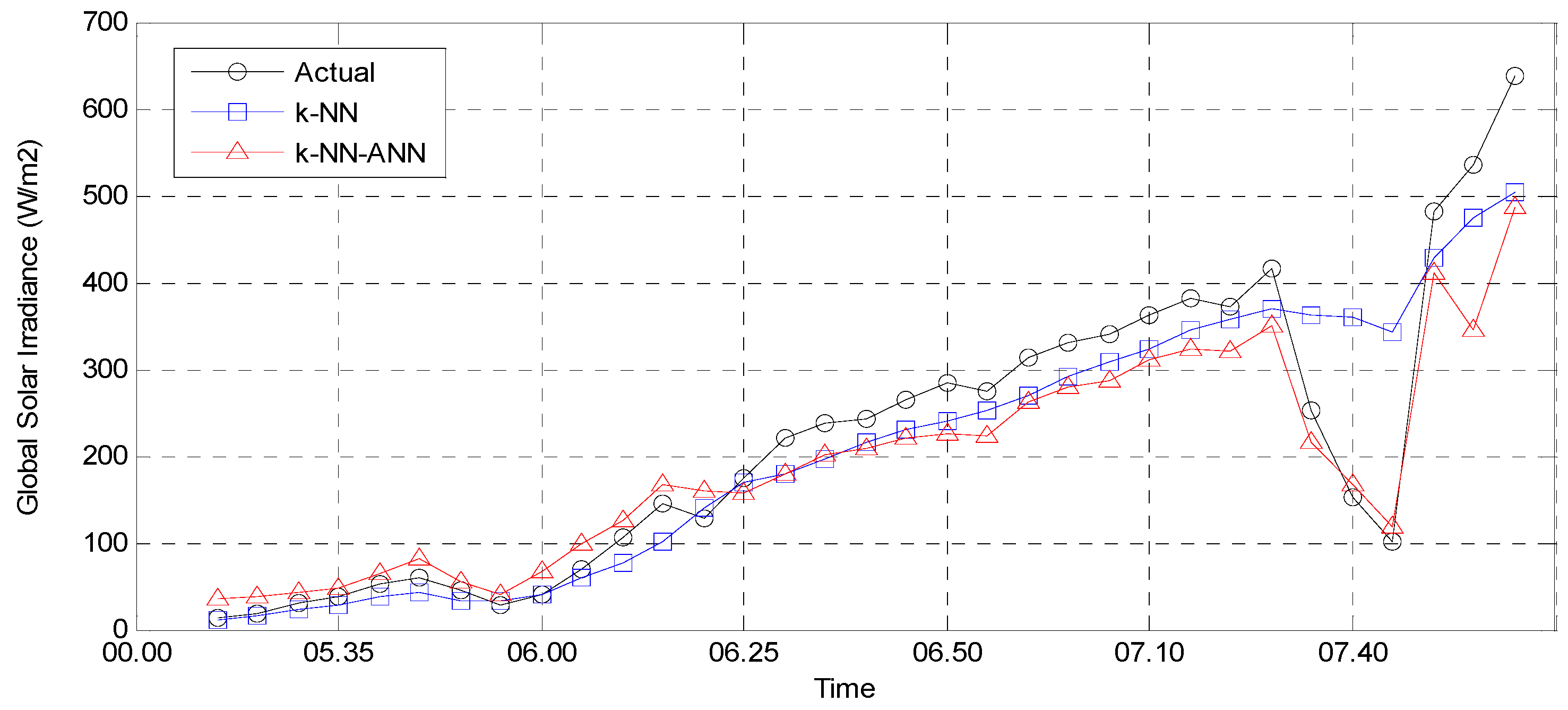
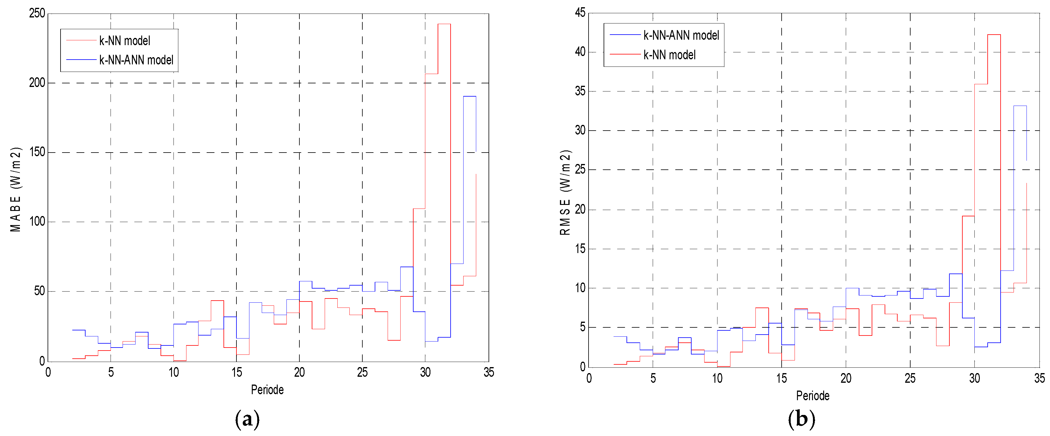
- This paper utilises k-NN-ANN modelling to determine the d-dimensional features and n-dimensional distances. The results demonstrate that the results of the k-NN-ANN model are closely matched with the actual data, and are better than data obtained from k-NN models.
Author Contributions
Conflicts of Interest
References
- Yang, H.T.; Yang, P.C.; Huang, C.L. Optimization of Unit Commitment Using Parallel Structures of Genetic Algorithm. In Proceedings of the 1995 International Conference on Energy Management and Power Delivery, Singapore, 21–23 November 1995.
- Chiang, C.-T.; Lee, Y.-S.; Li, X.R.; Liao, C.-C. A RSCMAC Based Forecasting for Solar Irradiance from Local Weather Information. In Proceedings of the WCCI 2012 IEEE World Congress on Computational Intelligence, Brisbane, Australia, 10–15 June 2012.
- Hocaoğlu, F.O. Stochastic approach for daily solar radiation modeling. Sol. Energy 2011, 85, 278–287. [Google Scholar] [CrossRef]
- Pedro, H.T.C.; Coimbra, C.F.M. Nearest-neighbor methodology for prediction of intra-hour global horizontal and direct normal irradiances. Renew. Energy 2015, 80, 770–782. [Google Scholar] [CrossRef]
- Salcedo-Sanz, S.; Casanova-Mateo, C.; Munoz-Marí, J.; Camps-Valls, G. Prediction of Daily Global Solar Irradiation Using Temporal Gaussian Processes. IEEE Geosci. Remote Sens. Lett. 2014, 11, 1936–1940. [Google Scholar] [CrossRef]
- Yang, D.; Sharmaa, V.; Ye, Z.; Lim, L.I.; Zhao, L.; Aryaputera, A.W. Forecasting of global horizontal irradiance by exponential smoothing using decompositions. Energy 2015, 81, 111–119. [Google Scholar] [CrossRef]
- Yang, D.; Ye, Z.; Lim, L.H.I.; Dong, Z. Very short term irradiance forecasting using the lasso. Sol. Energy 2015, 114, 314–326. [Google Scholar] [CrossRef]
- Licciardi, G.A.; Dambreville, R.; Chanussot, J.; Dubost, S. Spatiotemporal Pattern Recognition and Nonlinear PCA for Global Horizontal Irradiance Forecasting. IEEE Geosci. Remote Sens. Lett. 2015, 12, 284–288. [Google Scholar] [CrossRef]
- Amrouche, B.; Le Pivert, X. Artificial neural network based daily local forecasting for global solar radiation. Appl. Energy 2014, 130, 333–341. [Google Scholar] [CrossRef]
- Wong, L.T.; Chow, W.K. Solar radiation model. Appl. Energy 2001, 69, 191–224. [Google Scholar] [CrossRef]
- Voyant, C.; Paolia, C.; Musellia, M.; Niveta, M.-L. Multi-horizon Irradiation Forecasting for Mediterranean Locations Using Time Series Models. Energy Procedia 2014, 57, 1354–1363. [Google Scholar]
- Lorenz, E.; Hurka, J.; Heinemann, D.; Beyer, H.G. Irradiance Forecasting for the Power Prediction of Grid-Connected Photovoltaic Systems. IEEE J. Sel. Top. Appl. Earth Obs. Remote Sens. 2009, 2, 2–10. [Google Scholar] [CrossRef]
- Wang, F.; Mi, Z.; Su, S.; Zhao, H. Short-Term Solar Irradiance Forecasting Model Based on Artificial Neural Network Using Statistical Feature Parameters. Energies 2012, 5, 1355–1370. [Google Scholar] [CrossRef]
- Mellit, A.; Pavan, A.M. A 24-h forecast of solar irradiance using artificial neural network: Application for performance prediction of a grid-connected PV plant at Trieste Italy. Sol. Energy 2010, 84, 807–821. [Google Scholar] [CrossRef]
- Hammer, A.; Heinemann, D.; Lorenz, E.; Luckehe, B. Short-Term Forecasting of Solar Radiation: A Statistical Approach Using Satellite Data. Sol. Energy 1999, 67, 139–150. [Google Scholar] [CrossRef]
- Xiao, C.; Chaovalitwongse, W.A. Optimization Models for Feature Selection of Decomposed Nearest Neighbor. IEEE Trans. Syst. Man Cybern. Syst. 2016, 46, 2168–2216. [Google Scholar] [CrossRef]
- Perez, R.; Kivalov, S.; Schlemmer, J.; Hemker, K., Jr.; Renné, D.; Hoff, T.E. Validation of short and medium term operational solar radiation forecasts in the US. Sol. Energy 2010, 84, 2161–2172. [Google Scholar] [CrossRef]
- Marquez, R.; Coimbra, C.F.M. Forecasting of global and direct solar irradiance using stochastic learning methods, ground experiments and the NWS database. Sol. Energy 2011, 85, 746–756. [Google Scholar] [CrossRef]
- Martin, L.; Zarzalejo, L.F.; Polo, J.; Navarro, A.; Marchante, R.; Cony, M. Prediction of global solar irradiance based on time series analysis: Application to solar thermal power plants energy production planning. Sol. Energy 2010, 84, 1772–1781. [Google Scholar] [CrossRef]
- Boata, R.S.; Gravila, P. Functional fuzzy approach for forecasting daily global solar irradiation. Atmos. Res. 2012, 112, 79–88. [Google Scholar] [CrossRef]
- Dambreville, R.; Blanc, P.; Chanussot, J.; Boldo, D. Very short term forecasting of the Global Horizontal Irradiance using a spatio-temporal autoregressive model. Renew. Energy 2014, 72, 291–300. [Google Scholar] [CrossRef]
- Diagne, M.; David, M.; Lauret, P.; Boland, J.; Schmutz, N. Review of solar irradiance forecasting methods and a proposition for small-scale insular grids. Renew. Sustain. Energy Rev. 2013, 27, 65–76. [Google Scholar] [CrossRef]
- Zeng, J.; Qiao, W. Short-term solar power prediction using a support vector machine. Renew. Energy 2013, 52, 118–127. [Google Scholar] [CrossRef]
- Dong, Z.; Yang, D.; Reindl, T.; Walsh, W.M. Short-term solar irradiance forecasting using exponential smoothing state space model. Energy 2013, 55, 1104–1113. [Google Scholar] [CrossRef]
- Ren, Y.; Suganthan, P.N.; Srikanth, N. A Comparative Study of Empirical Mode Decomposition-Based Short-Term Wind Speed Forecasting Methods. IEEE Trans. Sustain. Energy 2015, 6, 236–244. [Google Scholar] [CrossRef]
- Mellit, A.; Benghanem, M.; Bendekhis, M. Artificial Neural Network Model for Prediction Solar Radiation Data: Application for Sizing Stand-Alone Photovoltaic Power System. In Proceedings of the 2005 IEEE Power Engineering Society General Meeting, San Francisco, CA, USA, 12–16 June 2005.
- Farhad, S.G.; Khaze, S.R.; Malekl, I. A new Approach in Bloggers Classification with Hybrid of K-Nearest Neighbor and Artificial Neural Network Algorithms. Indian J. Sci. Technol. 2015, 8, 237–246. [Google Scholar]
- Zhang, Y.; Wang, J. GEFCom2014 Probabilistic Solar Power Forecasting based on k-Nearest Neighbor and Kernel Density Estimator. In Proceedings of the 2015 IEEE Power & Energy Society General Meeting, Denver, CO, USA, 26–30 July 2015.
- López, G.; Batlles, F.J.; Tovar-Pescador, J. Selection ofinput parameters to model direct solar irradiance by using artificial neural networks. Energy 2005, 30, 1675–1684. [Google Scholar] [CrossRef]
- Anil, K.; Jain, J.; Mao, K. Mohiuddin, Artificial Neural Networks: A Tutorial. Computer 1996, 29, 31–44. [Google Scholar]
- Wu, B.; Li, K.; Yang, M.; Lee, C.-H. A Reverberation-Time-Aware Approach to Speech Dereverberation Based on Deep Neural Networks. IEEE/ACM Trans. Audio Speech Lang. Process. 2017, 25, 102–111. [Google Scholar] [CrossRef]


| No. | Station | Angle (°) | Distance (d) | Coordinate (xi, yi) |
|---|---|---|---|---|
| 1 | A | 0 | 8.3 | (8.3, 0) |
| 2 | B | 36 | 10.5 | (8.5, 6.2) |
| 3 | C | 93 | 10.8 | (−0.6, 10) |
| 4 | D | 140 | 10.5 | (−8, 6.7) |
| 5 | E | 180 | 10 | (−10, 0.1) |
| 6 | F | 250 | 4.3 | (−5.5, −5) |
| 7 | G | 280 | 5.4 | (1, −5.3) |
| 8 | H | 310 | 9.1 | (5.8, −7) |
| 9 | S | 0 | 0 | (0.1, 0.1) |
| Time | Station (x, y) * | ||||||||
|---|---|---|---|---|---|---|---|---|---|
| ST-S (0.1, 0.1) | ST-A (8.3, 0) | ST-B (8.5, 6.2) | ST-C (−0.6, 10) | ST-D (−8, 6.7) | ST-E (−10, 0.1) | ST-F (−5.5, −5) | ST-G (1, −5.3) | ST-H (5.8, −7) | |
| 5:20 | 11 | 11 | 11 | 11 | 10 | 10 | 10 | 11 | 11 |
| 5:25 | 15 | 15 | 15 | 15 | 15 | 15 | 15 | 15 | 15 |
| 5:30 | 22 | 22 | 22 | 22 | 22 | 22 | 22 | 22 | 22 |
| 5:35 | 27 | 29 | 27 | 25 | 24 | 25 | 27 | 28 | 30 |
| 5:40 | 37 | 39 | 37 | 33 | 33 | 35 | 38 | 39 | 41 |
| 5:45 | 42 | 44 | 44 | 42 | 41 | 40 | 41 | 42 | 43 |
| 5:50 | 33 | 35 | 38 | 38 | 35 | 31 | 30 | 31 | 31 |
| 5:55 | 32 | 32 | 31 | 31 | 31 | 32 | 32 | 32 | 32 |
| 6:00 | 40 | 41 | 36 | 33 | 35 | 40 | 44 | 44 | 46 |
| 6:05 | 59 | 61 | 53 | 45 | 48 | 57 | 65 | 67 | 70 |
| 6:10 | 77 | 82 | 76 | 67 | 66 | 72 | 79 | 83 | 88 |
| 6:15 | 101 | 106 | 100 | 91 | 90 | 95 | 103 | 107 | 111 |
| 6:20 | 139 | 132 | 113 | 110 | 127 | 148 | 160 | 155 | 155 |
| 6:25 | 169 | 152 | 133 | 140 | 165 | 189 | 195 | 183 | 178 |
| 6:30 | 179 | 158 | 153 | 172 | 194 | 204 | 197 | 181 | 170 |
| 6:35 | 197 | 186 | 184 | 196 | 207 | 211 | 206 | 197 | 191 |
| 6:40 | 216 | 200 | 202 | 221 | 234 | 235 | 225 | 213 | 203 |
| 6:45 | 230 | 217 | 219 | 236 | 246 | 246 | 237 | 226 | 218 |
| 6:50 | 240 | 229 | 233 | 248 | 256 | 254 | 245 | 235 | 228 |
| 6:55 | 252 | 238 | 243 | 263 | 272 | 269 | 256 | 245 | 235 |
| 7:00 | 269 | 256 | 260 | 278 | 287 | 285 | 274 | 263 | 254 |
| 7:05 | 292 | 275 | 275 | 294 | 310 | 314 | 304 | 290 | 280 |
| 7:10 | 308 | 290 | 290 | 310 | 326 | 330 | 320 | 305 | 295 |
| 7:15 | 324 | 302 | 302 | 327 | 347 | 351 | 338 | 321 | 307 |
| 7:20 | 345 | 322 | 320 | 345 | 366 | 373 | 361 | 343 | 330 |
| 7:25 | 357 | 334 | 334 | 360 | 381 | 385 | 372 | 354 | 340 |
| 7:35 | 370 | 351 | 354 | 379 | 394 | 395 | 380 | 365 | 351 |
| 7:40 | 362 | 331 | 334 | 371 | 397 | 400 | 380 | 355 | 336 |
| 7:45 | 360 | 323 | 327 | 372 | 402 | 405 | 380 | 351 | 327 |
| 7:50 | 344 | 316 | 328 | 367 | 385 | 378 | 352 | 329 | 310 |
| 7:55 | 427 | 414 | 414 | 429 | 440 | 443 | 436 | 426 | 418 |
| 8:00 | 475 | 457 | 450 | 467 | 486 | 497 | 492 | 478 | 469 |
| Model Error Indicators | k-NN | k-NN-ANN |
|---|---|---|
| MABE (W/m2) | 44 | 42 |
| RMSE (W/m2) | 251 | 242 |
© 2017 by the authors. Licensee MDPI, Basel, Switzerland. This article is an open access article distributed under the terms and conditions of the Creative Commons Attribution (CC BY) license ( http://creativecommons.org/licenses/by/4.0/).
Share and Cite
Chen, C.-R.; Kartini, U.T. k-Nearest Neighbor Neural Network Models for Very Short-Term Global Solar Irradiance Forecasting Based on Meteorological Data. Energies 2017, 10, 186. https://doi.org/10.3390/en10020186
Chen C-R, Kartini UT. k-Nearest Neighbor Neural Network Models for Very Short-Term Global Solar Irradiance Forecasting Based on Meteorological Data. Energies. 2017; 10(2):186. https://doi.org/10.3390/en10020186
Chicago/Turabian StyleChen, Chao-Rong, and Unit Three Kartini. 2017. "k-Nearest Neighbor Neural Network Models for Very Short-Term Global Solar Irradiance Forecasting Based on Meteorological Data" Energies 10, no. 2: 186. https://doi.org/10.3390/en10020186