Fourier, Wavelet, and Hilbert-Huang Transforms for Studying Electrical Users in the Time and Frequency Domain ^†

Abstract

The analysis of electrical signals is a pressing requirement for the optimal design of power distribution. In this context, this paper illustrates how to use a variety of numerical tools, such as the Fourier, wavelet, and Hilbert-Huang transforms, to obtain information relating to the active and reactive power absorbed by different types of users. In particular, the Fourier spectrum gives the most important frequency components of the electrical signals, and the wavelet analysis highlights the non-stationarity of those frequency contributions, whereas the Hilbert-Huang transform, by means of the Empirical Mode Decomposition, provides a more complete spectrum of frequencies.

1. Introduction

In the era of smart grids, the monitoring of power systems is needed for several purposes. It is used to detect failures in the electrical network, to underline the contributions of the distributed generators on the dynamic behavior of the whole system, and, more generally, to optimize the power distribution [1,2]. Nevertheless, the monitoring is not trivial, due to the massive use of non-linear loads and electronic-based equipment in residential, commercial, and industrial plants. In order to control the operation of the electrical lines, it is very important to implement and develop both on-line and off-line systems which are able to check the power fluctuations, related to the power absorbed by the numerous loads of each user. It is important to note that a disadvantage of this system is the large amount of data which has to be managed during the monitoring process. Even though several researchers have focused their attention on compacting the electrical information [3,4,5], a more detailed investigation on this state of the art process highlights that the compression of the signal waveform is not as mature as for speech, image, and video compression [6]. The complexity depends on the characteristics of the electrical signals of the modern equipment, which are related to the different loads (static, rotating, power electronics-based, and so on) and generators (deterministic-based, stochastic-based). The consequence of the diversity of the electrical loads induces the same electrical signals, which are nonlinear, non-stationary, and non-periodic.

In order to deal with this large amount of data and to manage the electrical signals, two main categories of mathematical tools, based on compression techniques, have been used: lossless techniques [7,8,9] and lossy algorithms [3,10,11,12]. Reference [6] reports a comparison of these tools (see Table I of [6]), based on the compression ratio and the distortion values. However, the appropriate choice of the technique to treat an electrical signal, is not trivial. In fact, as an example, if the electrical signal is linear and stationary, traditional mathematical tools, like the standard Fast Fourier transform (FFT), can be the correct analysis method. Vice versa, in the presence of electrical signals that deviate from linear and periodic behavior, different and more complex tools are necessary, in order to correctly characterize the electrical power behaviors. In recent years, the Wavelet Transform (WT) has been used increasingly often for several different issues related to power systems at every level. In [13], the authors study the modal parameters of power systems in order to analyze the origin of the small signal oscillations, thanks to the continuous WT that is able to detect the damping and frequency of the critical modes. Moreover, this approach uses the FFT to calculate the convolution integral of the continuous WT, in order to reduce the computational burden. The WT is also employed for the fault location and the power quality analysis in electric power systems [14], where a combination of several mathematical tools is proposed, on the basis of behavioral indexes, neural networks, statistics, and WT. In addition to the WT, the Hilbert-Huang Transform (HHT) is an effective tool for studying the non-stationary phenomena of power systems. In [15], the authors propose an iterative HHT to study the power quality waveforms in the presence of a sudden transition. Moreover, to discriminate the correct instant, they also use the Symbolic Aggregate ApproXimation. HHT, together with the discrete WT, is also used to analyze the power system areas with coherent generator groups, therefore in no-fault conditions [16].

In this framework, the WT [12,13,14,15,16,17] and the Empirical Mode Decomposition (EMD) deriving from the calculation of the HHT [18,19] were also used with success, in order to determine the properties of non-linear, non-stationary, and non-periodic electrical signals of passive or active distribution lines (i.e., in the absence or presence of renewable energy sources, respectively). These tools, together with the FFT, allow a complete analysis of those signals, both in time and frequency domain.

The WT, specifically, evidences the non-stationarity of the signals [17,20]. In the distribution lines, WT was used to analyze the absorbed power in anomalous conditions [12], and to characterize different typologies of electrical users [21].

In addition, the HHT-EMD produces a description of the behavior of different kinds of signals that are typically nonlinear [22,23,24,25], overcoming the limitations of the FFT analysis, which is able to quantitatively describe signals with linear, stationary, and periodic characteristics. The efficiency of the HHT analysis of electrical power signals has already been tested, by comparing the HHT-based results and the FFT-based results, both for seasonal periods [26] and for long periods [19]. For the sake of completeness, when both the non-linearity and the non-stationarity are present, the Duffing equation [27] is an effective tool for investigating the electrical behavior of distribution lines.

This paper, in contrast to the previous literature and [21], which describes the FFT and WT analysis of the active power, presents a complete and deep methodology, based on the FFT, WT, and HHT-EMD analysis of both active and reactive power. The dataset derives from measured data of distribution lines, feeding different typologies of users (private residences, groceries, marketing retails, general services, restaurants). We also want to emphasize that, whereas in our previous work [19] we used FFT, WT, and HHT-EMD tools to study the different electrical behaviors of the active and passive distribution lines, here we use the same tools to highlight the different electrical behavior of end-users belonging to different typologies, with the aim of characterizing the end-user.

The paper is organized as follows. Section 2 describes the theoretical background, illustrating both the WT and the HHT; data under investigation are presented in Section 3; Section 4 discusses the numerical results after having processed our dataset by means of FFT, WT, and HHT; lastly, Section 5 is devoted to the conclusions.

2. Theoretical Framework

In this Section, we present the numerical methods used for the analysis of both the active and reactive power of the electrical users.

In particular, we firstly introduce the WT used to characterize signals in the time-frequency domain, pointing out the non-stationary behaviors. Secondly, the EMD based on the HHT formalism is presented, in order to correctly describe the non-linear behavior of these kinds of signals.

2.1. Wavelet Transform

The continuous wavelet transform $W(u,s)$ of a time-domain signal $x(t)$ is a linear function, defined as:

$$W(u,s)=\frac{1}{\sqrt{s}}{\displaystyle \underset{-\infty }{\overset{\infty }{\int }}x(t)\mathsf{\psi }*\left(\frac{t-u}{s}\right)dt}$$

(1)

where s and u are the scale and translation parameters of the mother wavelet $\mathsf{\psi }(t)$, that defines the wavelet family function as:

$${\mathsf{\psi }}_{u,s}(t)=\frac{1}{\sqrt{s}}\mathsf{\psi }\left(\frac{t-u}{s}\right)$$

(2)

The following complex Morlet mother wavelet has been utilized in this paper:

$${\mathsf{\psi }}_{u,s}=\frac{1}{\sqrt{s\pi f_B}}{e}^{j2\pi f_C\left(\frac{t-u}{s}\right)}{e}^{-\left(\frac{t-u}{s}\right)/f_B}$$

(3)

where f_B and f_C are two characteristic parameters. After setting the dimension N of the scale set {s}, the optimal scale set {s}_{i = 1, …, N} for the WT have been found, adopting the method reported in Reference [28,29,30].

2.2. HHT and EMD

Given a time-domain signal X(t), the HHT-based approach provides a calculation of the Hilbert transform Y(t) = H{X(t)}:

$$Y(t)=\frac{1}{\pi }P{\displaystyle \underset{-\infty }{\overset{\infty }{\int }}\frac{X(t\prime )}{t-t\prime }dt\prime }$$

(4)

where P represents the principal value. Instead, the Hilbert complex extension of X(t) is constituted by the analytical signal associated to X(t), $Z\left(t\right)=X\left(t\right)+jY\left(t\right)=X\left(t\right)+jH\left\{X(t)\right\}=a\left(t\right)e^{j\mathsf{\theta }\left(t\right)}$, where j is the imaginary unit, whereas the amplitude a(t) and the phase $\mathsf{\theta }(t)$ are represented by the following equations: $a(t)={\left[X^2(t)+Y^2(t)\right]}^{\frac{1}{2}}$ and $\mathsf{\theta }(t)=\arctan \frac{Y(t)}{X(t)}$, respectively. Considering the application of the stationary phase method to the Fourier transform F(ω) of Z(t), it yields $\mathsf{\omega }(t)=d\mathsf{\theta }(t)/dt$, where ω(t) is the instantaneous angular frequency [31]. By applying the methodology proposed in [18], and finalized to the EMD, the signal X(t) can be considered as a finite collection of single characteristic intrinsic modes, defined as Intrinsic Mode Functions (IMFs), i.e., $X(t)={\displaystyle \sum _{l=1}^N{c}_l(t)}+r_N(t)$, where $c_l(t)$ are the time-dependent IMFs with variable amplitude and $r_N(t)$ is the non-oscillatory residue term, due to the sifting process. The number of oscillations of the IMFs is related to their order, reducing the first, as the second increases. This effect is due to the algorithm employed for the iterative extractions of the IMFs. As it will be shown later, each iteration of EMD generates a new signal, obtained as the difference between the original signal and the mean value of the envelope curves, of its local maximum and minimum values.

For each IMF $c_l(t)$, having a characteristic angular frequency ${\mathsf{\omega }}_l(t)$, the complex representation can be written as:

$$z_l(t)=c_l(t)+j\frac{1}{\pi }P{\displaystyle \underset{-\infty }{\overset{\infty }{\int }}\frac{c_l(t\prime )}{t-t\prime }dt\prime }=a_l(t)e^{j{\mathsf{\theta }}_l(t)}$$

(5)

where $a_l(t)$ is the amplitude of $z_l(t)$, while ${\mathsf{\theta }}_l(t)={\displaystyle \int {\mathsf{\omega }}_l(t)dt}$, $l=1,2,\mathrm{...},N$.

Furthermore, the amplitude X(t) of an electrical signal expanded in a Fourier series, thus highlighting the IMF components, has the following form:

$$X\left(t\right)=Re\left\{{\displaystyle \sum }_{l=i}^N{z}_l\left(t\right)\right\}=Re\left\{{\displaystyle \sum }_{l=i}^N{a}_l\left(t\right)e^{j{\mathsf{\theta }}_l\left(t\right)}\right\}=Re\left\{{\displaystyle \sum }_{l=i}^N{a}_l\left(t\right)e^{2\mathsf{\pi }j{\displaystyle \int }{f}_l\left(t\right)}\right\}$$

(6)

where Re is the real part, and $f_l(t)={\mathsf{\omega }}_l(t)/2\pi$ is the instantaneous frequency of the l-th IMF, whereas the residue $r_N(t)$ is neglected, for instance when it is a monotonic function, which does not allow any extraction of IMFs.

In this paper, the proposed methodology is applied to two time-domain signals: the active power P(t) and the reactive power Q(t). Consequently, the Hilbert transform defined in Equation (4), and the Fourier representation of Equation (6), are expressed in terms of either P(t) or of Q(t). Equation (6) is the Hilbert amplitude spectrum H(ω,t), also known as the Hilbert spectrum.

3. Description of the Data and Coherence Degree

The dataset under investigation is constituted by the active and reactive powers absorbed by 25 different users, grouped into five different typologies (restaurants, groceries, marketing retails, general services, private residences). The sampling time of the measurements was fixed at 15 min, and the overall period of recording was three months, from the 1st of December, 2014, to the 28th of February, 2015, covering 90 consecutive days with 96 samples per day (90 × 96 = 8640 samples recorded per user). In exceptional cases (less than 0.5%), the power measurements were not available in the dataset, thus we connected the external values via interpolation. In this regard, after comparing different kinds of interpolation, the average of the values observed in similar circumstances (same hours in different days) turned out to be the most reliable method.

The first step concerned the time-domain analysis of the measured data, in order to extract the main features of the active power absorbed by the users, such as the maximum power and the typical timing of the power request. This analysis allowed an evaluation of the similarity level of the five users belonging to the same user typology and, then, whether it could be possible to average their behaviors, in order to identify the sample user of that typology, or to consider whether one user is representative of each typology. Successively, in order to estimate the likeness between users of the same category, we calculated the spectral coherence between the power signals of each couple of users, for the same typology. The time-frequency coherence of two signals, x(t) and y(t), is a real-valued function, defined as:

$$C_{xy}(f)=\frac{{\left|S_{xy}(f)\right|}^2}{S_x(f)S_y(f)}$$

(7)

where $S_{xy}(f)$ is the cross-spectral density between x(t) and y(t), and $S_x(f)$ and $S_y(f)$ are the autospectral densities of x(t) and y(t), respectively. The values of the coherence always range from zero to one [32,33].

Table 1. Coherence Values between Active Power Signals.

Users	Coherence
	Restaurants	Groceries	Marketing Retails	General Services	Private Residences
#1–#2	0.9463	0.9365	0.8773	0.6653	0.9866
#1–#3	0.9661	0.9595	0.9655	0.6798	0.9952
#1–#4	0.9116	0.9310	0.8879	0.7033	0.9913
#1–#5	0.9375	0.9594	0.9382	0.7058	0.9225
#2–#3	0.9464	0.9609	0.9008	0.9961	0.9821
#2–#4	0.9324	0.9548	0.9302	0.9812	0.9870
#2–#5	0.9426	0.9825	0.9036	0.9718	0.9114
#3–#4	0.9194	0.9504	0.9005	0.9837	0.9879
#3–#5	0.9441	0.9684	0.9281	0.9751	0.9048
#4–#5	0.9300	0.9505	0.9112	0.9819	0.9320
	Average Coherence for Each User
#1	0.9404	0.9466	0.9172	0.6886	0.9739
#2	0.9419	0.9587	0.9030	0.9036	0.9668
#3	0.9440	0.9598	0.9237	0.9087	0.9675
#4	0.9234	0.9467	0.9075	0.9125	0.9746
#5	0.9386	0.9652	0.9203	0.9087	0.9177

shows the coherence values obtained by the Equation (7), including the average coherence of each user. The less coherent users for each typology are: restaurant #4, grocery #1, marketing retail #2, general services #1, and private residence #5.

Finally, our proposed time-frequency analysis was completed. We will first plot the time-domain power signals of a user for each typology, over the whole data acquisition period. Next, we report on the frequency-domain analysis, including the frequency spectrum obtained by means of FFT, the WT scalogram, and the HHT analysis.

4. Results and Discussion

4.1. Temporal Analysis of the Active and Reactive Power

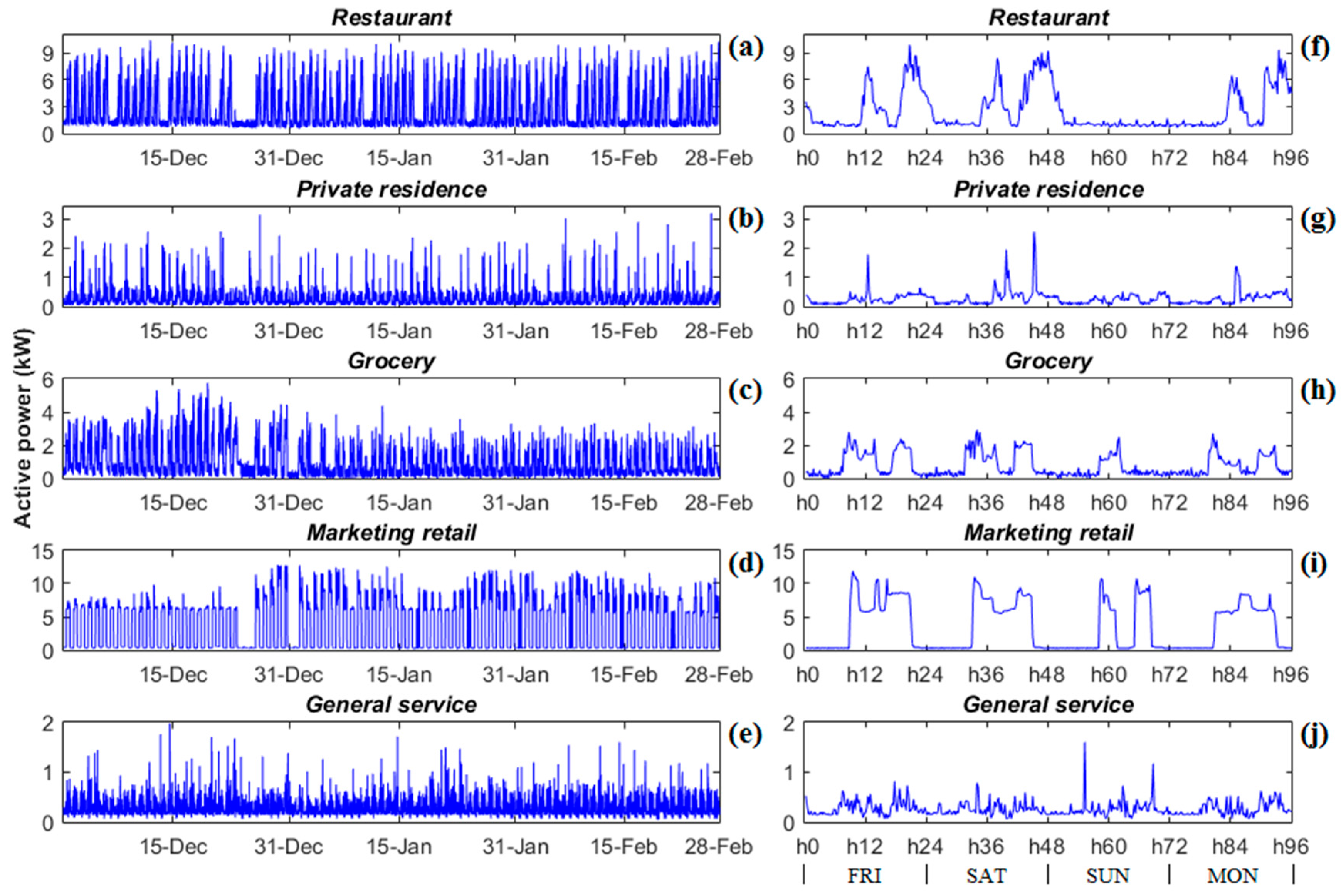
From the coherence analysis results, we have chosen one user which is the most representative of each typology. Figure 1a reports the active power absorbed by the user restaurant #2 in the trimester, whereas Figure 1f is a zoomed-in view of a 4-day interval, from a Friday to a Monday of February. As it can be seen, this specific user mainly absorbs power during two specific periods, lunch and dinner time, respectively. Moreover, it is almost always closed on Sundays. The diagram points out when the absorbed power is very low, corresponding to the closing days. The Christmas holidays are evidenced by the longest closing period.

User #1 is the reference for the category Private residence #1, and Figure 1b diagrams its active power (supply contract of 3 kW). A detailed forecasting of the absorbed power is impossible to obtain during the day, nevertheless, it is mainly concentrated during the day hours. As you can see, there is no appreciable difference in the absorbed power, with respect to the Christmas period, as occurred in the previous case.

Figure 1c reports the power absorbed by the user grocery #3, which has a 6 kW supply contract. The absorbed power is concentrated in two periods, the morning and the afternoon opening times. Sunday is the closing day. In addition, the time evolution of the power highlights, once again, a very low power request during the Christmas holidays.

Figure 1d shows the power absorbed by user #1 of the category marketing retail, with a 10 kW supply contract. The absorbed power is regular during the whole daytime, specifically from 9 a.m. to 9 p.m. It is evident that the retail establishment is usually open on Sundays, until the lunch break. Finally, the retail is closed during Christmas day and New Year’s day.

Figure 1e regards general service #2 (supply contract of 1.5 kW). The absorbed power is largely variable during the day, and it depends on the particular typology of the electrical load, including elevators, lights in common spaces, and so on, and therefore, the requested power is not predictable during the day.

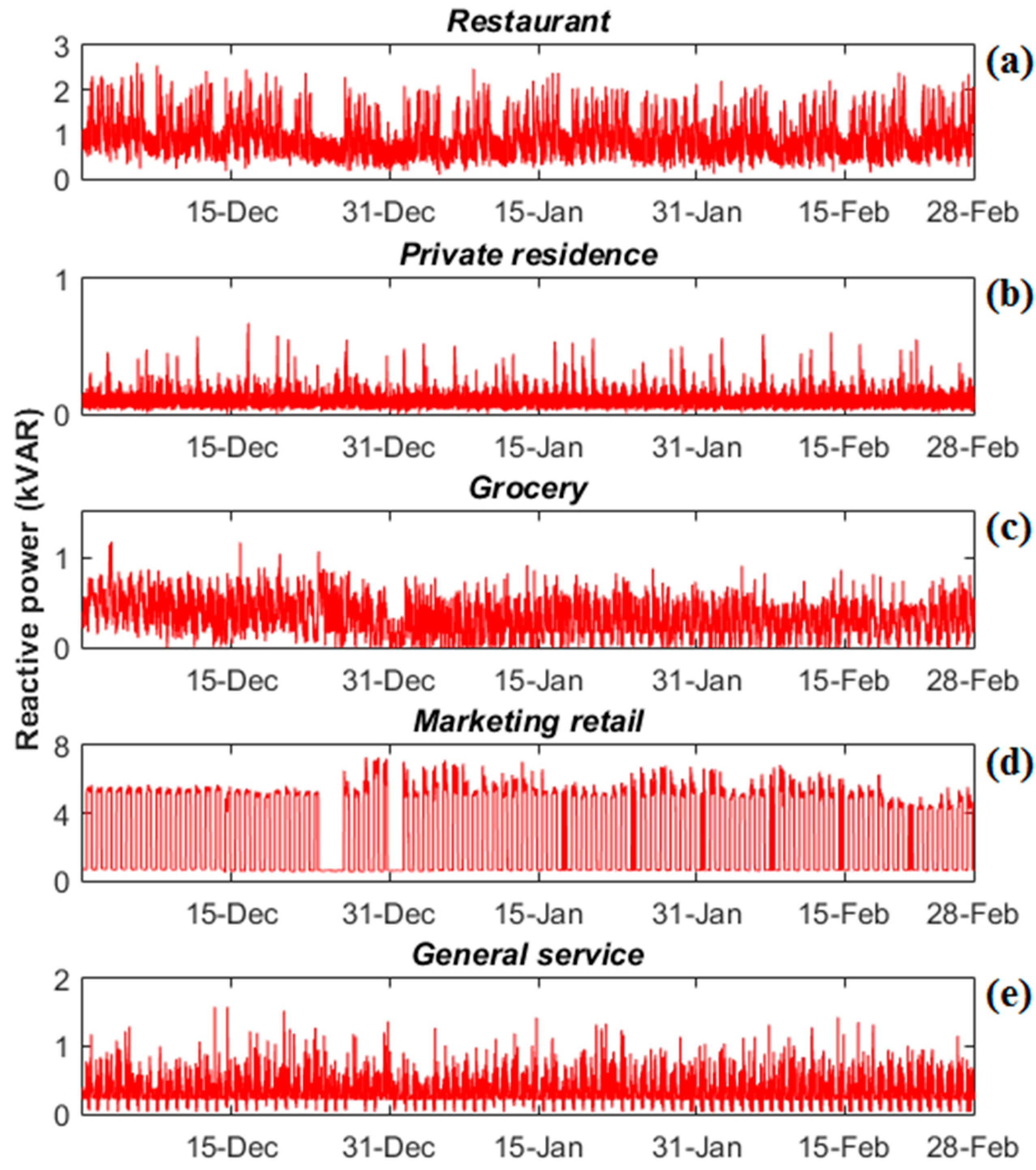
Figure 2 shows a similar study of the reactive power, for the same users analyzed above.

As expected, in the private residences, the reactive power contribution is very low, because there are loads absorbing a very low quantity of reactive power. Vice versa, restaurants and marketing retail establishments produce the most interesting users for the analysis of the reactive power, because their typical electrical loads are transformers and motors. In both cases, you can observe a power request during the day hours, whereas small values of reactive power are cyclically requested by the restaurant during the night.

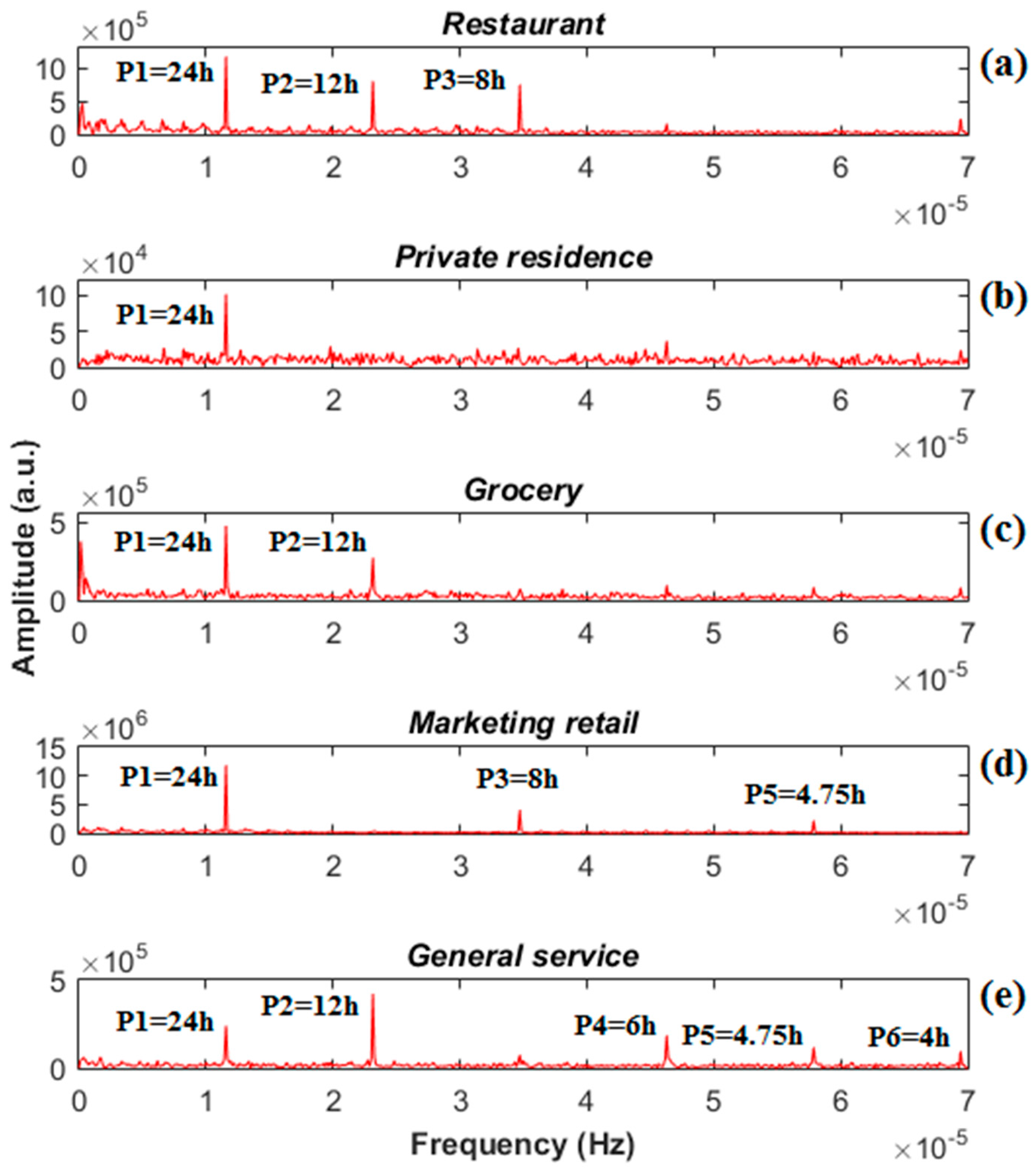
4.2. FFT Analysis

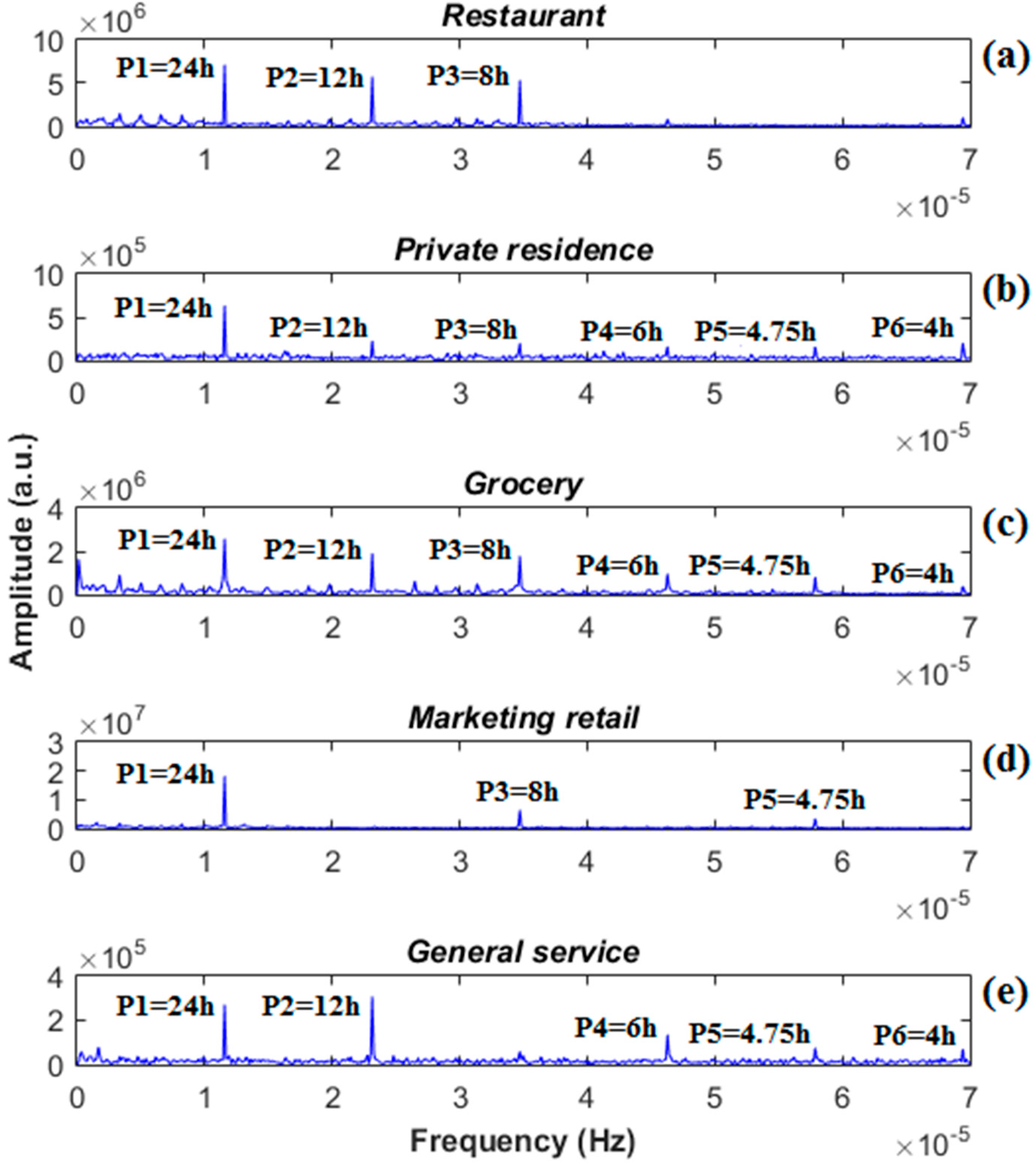
The Fourier spectrum of the first considered user (restaurant #2) shows the most important frequency components, which are at f₁ = 1.157 × 10⁻⁵ Hz, f₂ = 2.315 × 10⁻⁵ Hz, and f₃ = 3.472 × 10⁻⁵ Hz, corresponding to 24, 12, and 8 h, respectively, and are named P₁, P₂, and P₃, respectively, in Figure 3a. The Fourier spectrum of private residence #2 (see Figure 3b) highlights the contributions of P₁, P₂, P₃, P₄ (f₄ = 4.630 × 10⁻⁵ Hz, corresponding to 6 h), P₅ (f₅ = 5.787 × 10⁻⁵ Hz, corresponding to 4.75 h), and P₆ (f₆ = 6.944 × 10⁻⁵ Hz, corresponding to 4 h).

Figure 3c represents the Fourier spectrum of grocery #3, where the same peaks of the previous case are detected, without the peak P₆. In the case of marketing retail #1, the Fourier spectrum only contains the frequency components, P₁, P₃, and P₅ (see Figure 3d), related to the odd components of the Fourier spectrum. Frequency contributions of the general service #2 (Figure 3e) include P₁, P₂, P₄, P₅, and P₆.

When observing the Fourier analysis of the reactive power (see Figure 4), it becomes evident that the main frequency modes are the same for the related user of the active power spectrum, when the absorbed active and reactive powers are comparable. In our case, the only user which has a reactive power that is much lower than the active one, is the private residence (see Figure 1b and Figure 2b). In fact, the spectrum of the active and reactive power contains different frequency peaks, all of the harmonics of the spectrum for the active power, and only the first harmonic for the reactive power.

4.3. Wavelet Analysis

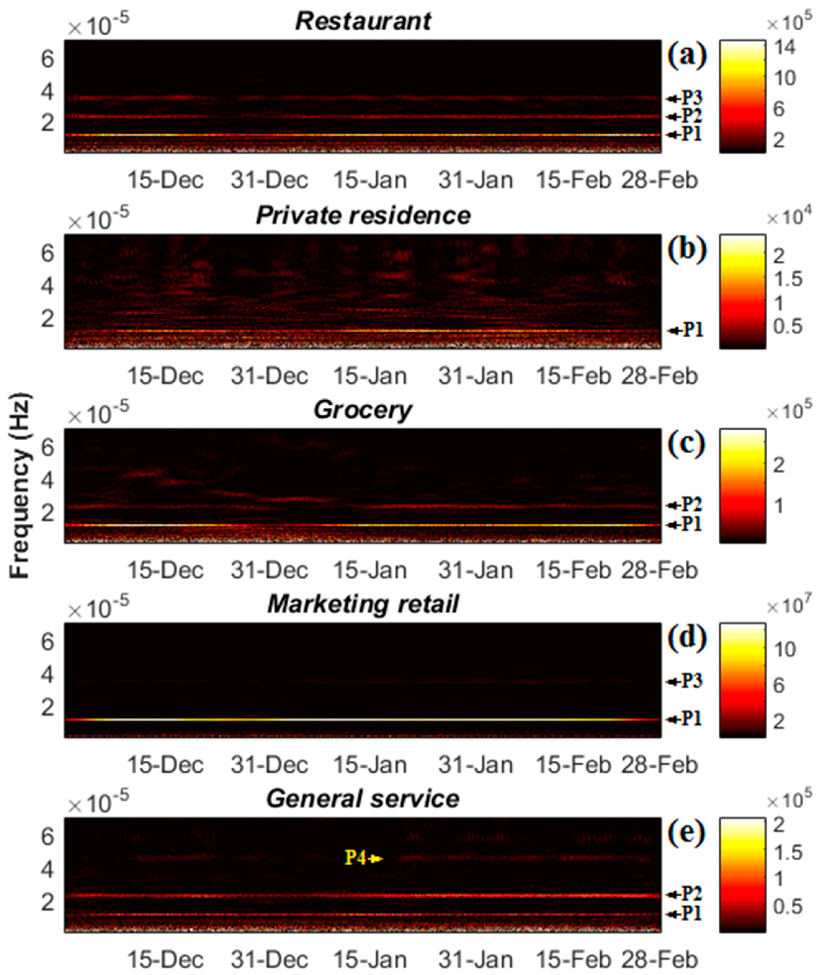
The WT analysis is an effective mathematical method for studying the non-stationary behavior of the electrical signals.

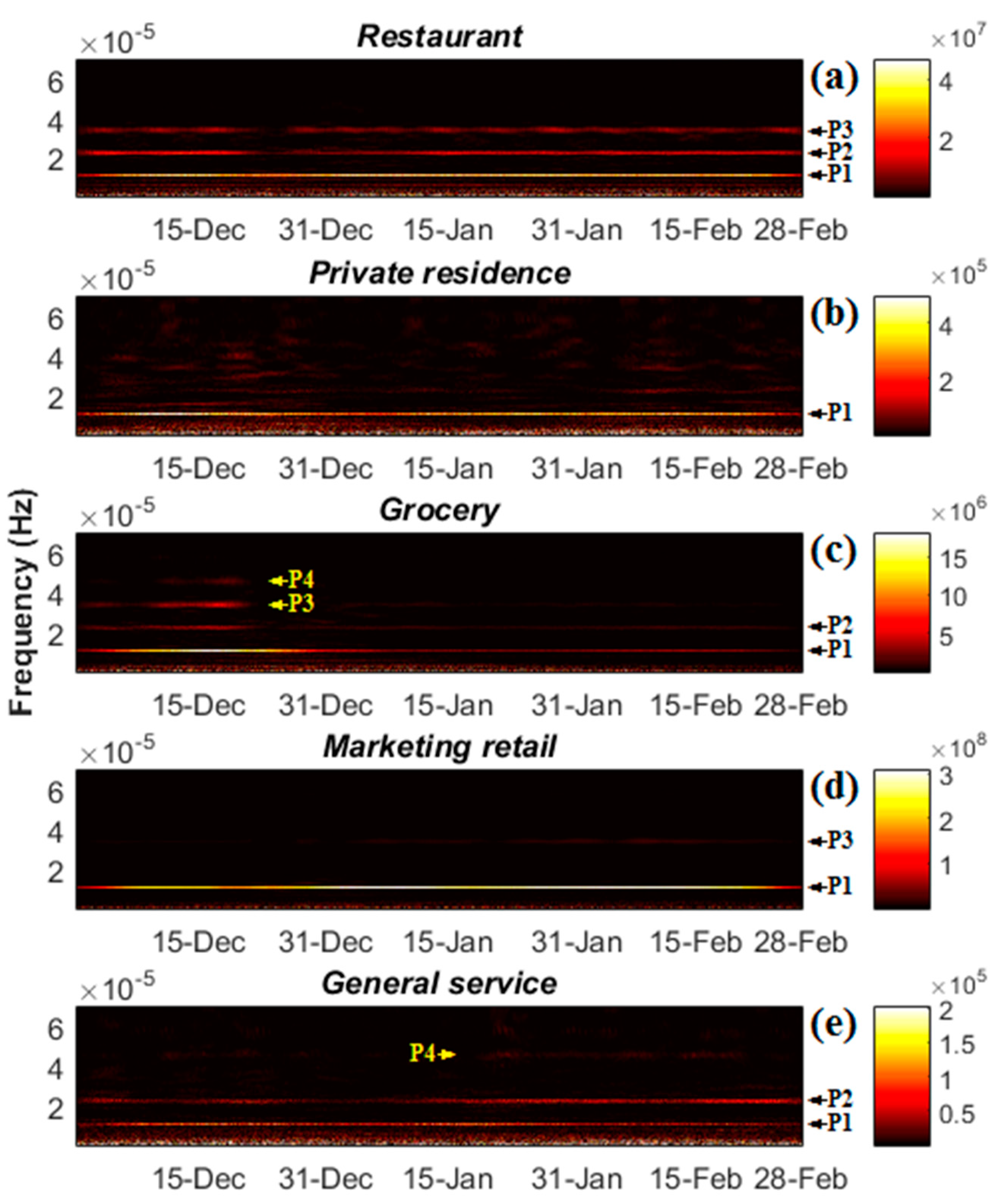
Figure 5 shows the WT scalogram of the active power for each user under study. In particular, Figure 5a is related to the restaurant, where P₁ and P₂ appear during the Christmas time, thus resulting in quasi-stationary modes. P₃ takes into account the closing days, highlighting an intermitting excitation mode. Figure 5b reports the WT analysis for the private residence, where it is observed that, apart from the stationary mode P₁, the other harmonics are less significant and discontinuous. Concerning the grocery user, Figure 5c shows that the relevant modes, P₁ and P₂, appear during the whole trimester, while the other modes are only present in December. Figure 5d points out that, in the case of the marketing retail, P₁ is the only stationary mode, and instead, P₃ and P₅ are low power and non-stationary modes. Finally, Figure 5e illustrates that the first two peaks of the general service are quasi-stationary modes, while P₄ is only present in the final acquisition period.

Figure 6 reports the WT analysis for the reactive power of the same users discussed above. In the case of the restaurant, the scalogram shows the stationarity of the P₁ mode; P₂ is quasi-stationary, whereas P₃ is attenuated with respect to the corresponding active power peak. Concerning the grocery, the P₁ mode is stationary; however, it is weak during the Christmas period, which is related to a different work organization of the user. Marketing retail and general service show frequency modes similar to those obtained in the active power analysis during the whole period. As expected, the WT scalogram of private residence confirms that the reactive power is almost negligible.

4.4. HHT Analysis

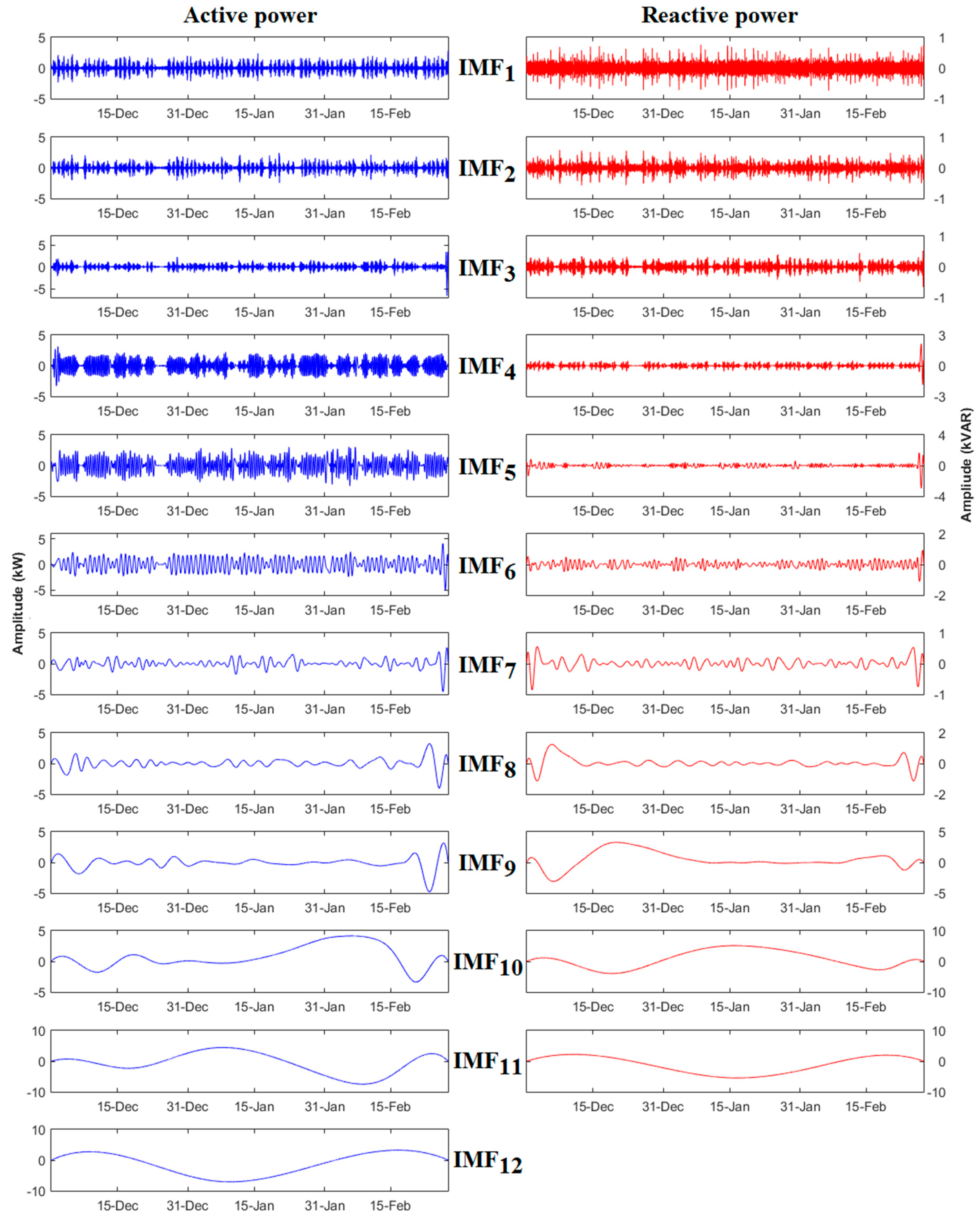
In order to provide an extensive analysis of the tools available to treat these particular electrical signals, characterized by the non-linear and non-stationary behavior, this section presents the results carried out by applying the HHT transform to one of the previous users (restaurant). Similar results are found for the other users (for the sake of brevity, not shown here).

In agreement with the EMD analysis on the basis of the HHT technique, the active power signal is decomposed into 12 IMFs (Figure 7, left column), whereas the reactive power one is decomposed into 11 IMFs (Figure 7, right column), for the whole sampling period. The IMFs are organized into a decreasing frequency order, due to the higher number of temporal oscillations of the signal, with respect to each successive iteration. The evidence that the active power shows a larger number of IMFs than the reactive power, is due to its higher non-linear behavior of the electrical signal under investigation. The frequencies of the intermediate IMFs, in our case #4–6, are very close to the ones found by performing the FFT analysis; all of the other IMFs have frequencies that do not correspond to those of the FFT harmonics.

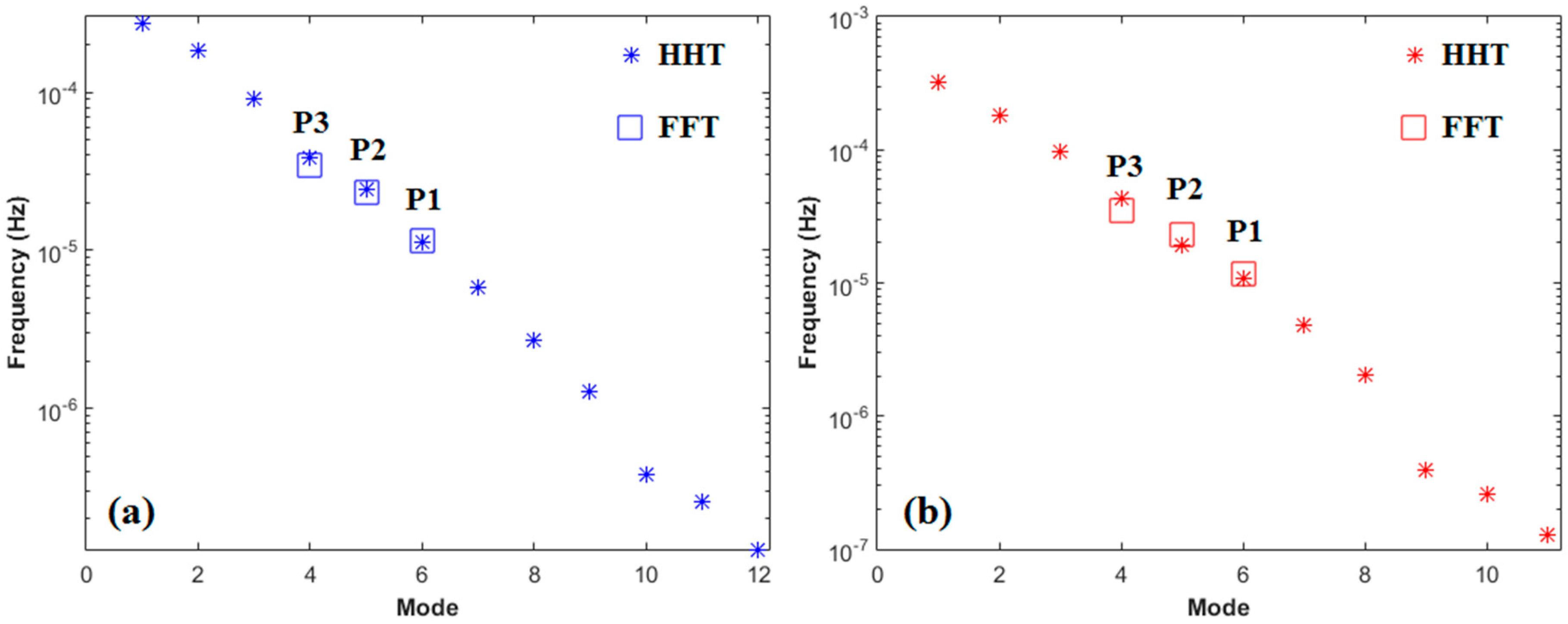
Figure 8a,b show the frequency peaks of the IMFs for active and reactive power, respectively. By comparing the HHT spectrum with the frequencies computed by the FFT, we observe that the HHT frequency range is much larger than the one found by using the FFT, and this means that the electrical signal of both the active and reactive power, is not periodical and non-linear. In fact, when comparing the excited modes found in the FFT (see Figure 3a and Figure 4a) and HHT spectrum, we observe that only the frequencies of the IMFs #4–6 for the active power and the reactive power, overlap with the frequency peaks computed by FFT analysis.

4.5. Discussion

From the results reported above, we find out that the FFT provides general information on the frequency behavior of both the active and reactive power. It is worth noting that the FFT is not the best method for studying non-stationary and non-linear signals acquired over a long period. In fact, the Fourier spectrum does not provide information on the time instant when the mode is excited, because it is time-independent. In the presence of non-stationary signals, the WT analysis overcomes this problem, because it computes the Fourier spectrum for different temporal windows. For example, Figure 5 and Figure 6 show that the frequency modes, for both the active and reactive power, are often not stationary during the whole period (three months), and the amplitude of the frequency peaks is not always constant.

FFT and WT are not able to extract all the frequency modes of the non-linear electrical signals, because they are covered by the noise and/or other frequency modes. From our analysis, the HHT transform has turned out to be a very useful tool for detecting all the frequency modes present in the active and reactive power of the case-studies. In fact, the information coming from the HHT is richer than that from the FFT, including a larger number of frequency components. Specifically, in the studied cases, for both active and reactive power, the modes of the FFT spectrum are contained in the central region of the HHT spectrum. The higher and lower frequency modes are not revealed when using the FFT and WT analyses, whereas the HHT spectrum includes the working modes at high and low frequency regimes, which are not revealed by the FFT analysis. The extraction of all the components is very important for several reasons. For example, many electrical loads contain magnetic parts, whose losses are frequency-dependent; therefore, it is only possible to correctly evaluate the losses if all the frequency components are known. Again, the magnetic parts of the electrical loads can be strongly nonlinear, and thus, the effects of the high frequency components cannot be negligible. Other similar examples of nonlinear and nonstationary signals can support the importance of the proposed analysis. Nonetheless, computational requirements for performing WT and HHT-EMD analysis are not significantly higher than the ones needed for a FFT calculation, and for this reason, the proposed methodology is effective and fast.

5. Conclusions

The analyses discussed above give a complete picture of the effectiveness of the different tools used to characterize the electrical signals. The different peculiarities of each analysis tool (FFT, WT, and HHT) imply that the choice of an appropriate method for the electrical signal to be studied is not trivial.

In conclusion, this paper shows that the HHT-EMD tool allows an extraction of the characteristic properties of the electrical signals, which are not found using the FFT and WT analyses; moreover, it can be used for both active and reactive powers. Finally, the frequency spectrum calculated via HHT-EMD is wider, with respect to the spectrum identified by means of the FFT and WT analyses. The reason for this is attributable to the non-periodical behavior of the electrical signals, connected to their strong deviation from linearity.