Review

Energy-Extended CES Aggregate Production: Current Aspects of Their Specification and Econometric Estimation

1
Sustainability Research Institute, School of Earth and Environment, University of Leeds, Leeds LS2 9JT, UK
2
Engineering Department, Calvin College, Grand Rapids, MI 49546, USA
3
MARETEC—Marine, Environment, and Technology Center, Environment and Energy Scientific Area, Department of Mechanical Engineering, Instituto Superior Técnico (IST), University of Lisbon, Avenida Rovisco Pais, 1 1049-001 Lisbon, Portugal
*
Author to whom correspondence should be addressed.
Energies 2017, 10(2), 202; https://doi.org/10.3390/en10020202
Submission received: 18 November 2016 / Accepted: 4 February 2017 / Published: 10 February 2017

Abstract

:
Capital–labour–energy Constant Elasticity of Substitution (CES) production functions and their estimated parameters now form a key part of energy–economy models which inform energy and emissions policy. However, the collation and guidance as to the specification and estimation choices involved with such energy-extended CES functions is disparate. This risks poorly specified and estimated CES functions, with knock-on implications for downstream energy–economic models and climate policy. In response, as a first step, this paper assembles in one place the major considerations involved in the empirical estimation of these CES functions. Discussions of the choices and their implications lead to recommendations for CES empiricists. The extensive bibliography allows those interested to dig deeper into any aspect of the CES parameter estimation process.

1. Introduction

1.1. The Growing Use of CES Aggregate Production Functions

Production functions seek to explain economic output arising from input factors of production, and are central to growth accounting (i.e., the study of the components of economic growth), empirical investigations versus economic theory, and macroeconomic modelling. For our purposes, we define aggregate production functions as those applied at sector [1,2] or economy-wide [3,4,5] levels.
The two most common aggregate production functions are the Cobb–Douglas (C-D) and Constant Elasticity of Substitution (CES) functions [6,7], as shown by the Google Scholar results illustrated in Figure 1. (Google Scholar was preferred to searching in Scopus or Web of Science, as it enabled access to wider “real-world” production function literature such as central bank reports). Their central position in macroeconomic models mean “these functions play an important role in the [government’s] economic forecasts and policy” ([8], p. 1).
The C-D function in its famous 1928 formulation [9] is given in Equation (1), which according to conventional economic theory ascribes economic output ( Y t ) to two primary factors—capital ( K t ) and labour ( L t ):
Y t = θ e λ t K t α L t β
where α and β are the elasticities of output ( Y t ) with respect to capital and labour, respectively (noting also typically α + β = 1 to meet constant returns-to-scale assumption), θ captures a scale parameter, e λ t is the exogenous Solow residual, i.e., the part of economic output not explained by the endogenous factors of production, and t is time relative to an initial year. λ is a parameter capturing (exogenous) productivity growth, as defined by Equation (2), where Y ˙ , K ˙ , and L ˙ are time derivatives of Y , K , and L , respectively.
λ   =   Y ˙ Y   α K ˙ K β L ˙ L
An important parameter in economics is the elasticity of substitution (σ), a measure of the ease by which one production factor (e.g., labour) may be substituted by another (e.g., capital). For aggregate production functions, it is most commonly measured by the Hicks Elasticity of Substitution (HES), as given in Equation (3), where Y / X i is the marginal productivity of input X i , and Y / X j is the marginal productivity of input X j . The HES is thus a measure of the curvature of the production function isoquant, or as Stern writes, the “difficulty of substitution” ([10], p. 80).
H E S i j = l n ( X i X j ) l n ( ( Y X i ) ( Y X j ) )
In a C-D function, the elasticity of substitution has a fixed unity value. This significant constraint is overcome by the CES function, introduced in 1956 by Solow [11], and subsequently generalized in the “ACMS” paper by Arrow, Chenery, Minhas and Solow [12] in 1961. The CES function in Equation (4) has δ as a share parameter, ρ as a substitution parameter (leading to the HES, σ = 1/(1 − ρ)), ν as a returns-to-scale parameter, θ as a scale parameter, and λ is (as before) the exogenous productivity growth parameter. The CES is therefore more flexible than the C-D function, with several special cases depending on the value of σ as noted by Arrow et al. [12]: Leontief (σ = 0), C-D (σ = 1) and Linear (σ = ) functions.
Y t = θ   e λ t [ δ K t ρ + ( 1 δ )   L t ρ ]   ν ρ
In an empirical study, historical time-series data (of the factors of production and economic output) is added to the functional form (e.g., Equation (4)) to form an analytical model, whose econometric estimation obtains values for the unknown CES function parameters. Solow’s 1957 US study [3] using the C-D function was the first time-series empirical study of its kind and “a landmark in the development of growth accounting” ([13], p. 1) that was followed by others including Arrow et al. [12] and Denison [14]. Whilst many studies follow this neo-classical C-D approach [4,15,16], many researchers—famously including Solow [3]—found that increases in capital and labour factors of production commonly explained only a minority of output growth, with the remainder ascribed to exogenous growth parameter λ . Abramovitz ([17], p. 11) described the unknown component of economic output (i.e., the Solow residual) as “a measure of our ignorance”, whilst Hulten ([18], p. 9) advocates it “covers many components, some wanted (such as the effects of technical and organizational innovation), others unwanted (such as measurement error, omitted variables, aggregation bias, and model misspecification)”. As a result, a focus on growth accounting (including the Solow residual) has remained a priority for researchers including Jorgenson [19], Denison [20] and Hulten [18,21].

1.2. Adding Energy as a Factor of Production

Neo-classical capital–labour aggregate production functions ignore the possible role of energy as a factor of production, since it is viewed as an intermediate product (of capital and labour), rather than a primary input. The 1970s oil crises focussed attention on the role of energy in economic growth, and thus provided an opportunity for researchers to add energy (E) as an input [22,23,24], typically amending the C-D function in Equation (1) to that shown in Equation (5):
Y t = θ e λ t K t α L t β E t γ
where γ is the elasticity of output with respect to energy, and α + β + γ = 1 to meet constant returns to scale assumption.
More recently, adding energy as a factor of production in aggregate production functions has regained popularity [25]. One possible reason is practicality, in that “increasing attention on the energy and environmental issues has evoked a revival of the relevant macroeconomic modelling” ([26], p. 793)—in other words, the effects of energy in an energy–economic model cannot be studied unless it is included as an endogenous factor of production. Another possible reason is the growing evidence base that energy is tightly linked to economic growth [27,28,29].
Energy (E) can be placed inside a nested CES function by augmenting Equation (4) as shown in Equation (6), with capital and labour in an inner (K-L) nest, and energy in an outer (KL_E) nest.
Y t = θ   e λ t [ δ [ ( δ 1   K t ρ 1 + ( 1 δ 1 ) L t ρ 1 ] ρ / ρ 1 + ( 1 δ ) E t ρ ] ν ρ
where ρ and ρ 1 are substitution parameters which lead to the inner nest σ 1 within the inner (K-L) nest and an outer nest σ between the inner (K-L) composite and energy (E). Our inner nest ( δ 1 , ρ 1 ) and inner-to-outer nest ( δ , ρ ) share and substitution parameter notation follows Henningsen and Henningsen [30]. For completeness and relevant to the “nesting” discussion in Section 3.3, with three factors of production (K, L, and E), the CES function has two other possible nests in addition to the KL(E) structure—EK(L) in Equation (7) and LE(K) in Equation (8):
Y t = θ   e λ t [ δ [ ( δ 1   E t ρ 1 + ( 1 δ 1 ) K t ρ 1 ] ρ / ρ 1 + ( 1 δ ) L t ρ ] ν ρ
Y t = θ   e λ t [ δ [ ( δ 1   L t ρ 1 + ( 1 δ 1 ) E t ρ 1 ] ρ / ρ 1 + ( 1 δ ) K t ρ ] ν ρ

1.3. Aim and Scope of Paper

Three propositions provide the rationale for our paper. First, capital–labour–energy CES aggregate production functions are important to macroeconomic models which inform climate and economic policy. Second, this places a due weight of responsibility on the CES empiricist to make the most appropriate choices regarding the many aspects of their econometric specification and estimation. It also places a responsibility on the “downstream” users of empirical CES study results, to be aware of such aspects and their implications. Third, though single aspect literature of CES production function theory and empirical usage [5,26,30,31,32,33,34] exists, without a succinct collation of the most important issues and options, analytical blindspots and poorly specified functions are more likely, which may have significant impacts on the estimated parameters, and ultimately energy policy.
In response, this paper comprises three novel components. First, we evaluate the proposition that CES functions have become the most important energy-extended aggregate production function in empirical use. Second, we assemble in one place the major aspects of the econometric specification and estimation for capital–labour–energy CES functions. Third, the merits of choices relating to these aspects are discussed, and recommendations made where evidence or consensus exists. Whilst the primary audience are those CES analysts involved in empirical studies, the succinct and accessible paper is open to all along the energy modelling-to-policy chain, including macroeconomic modellers and energy policymakers. The extensive bibliography is deliberate: permitting those interested to dig deeper into issues than space allows in this single journal paper.
The paper starts with a broader review the applications of C-D and CES aggregate production function studies in Section 2. This provides the context for the narrowing of focus in Section 3 to consider the specification of the empirical CES model: comprising the design of the function form and the input time-series datasets. Next, parameter estimation techniques are examined in Section 4, before recommendations and conclusions are given in Section 5.
Before we begin, a note on our study boundary. First, our focus is predominantly at the economy-wide (i.e., national) scale, though many aspects considered are also relevant to sectoral-level functions. Second, spatial constraints mean we cannot empirically test the collated aspects. Instead, this is undertaken by Heun et al. [35], which is an empirical complement to this landscape paper, where four key modelling choices are examined to establish the differences in resulting CES parameter values, and the potential effects on downstream energy policy. Third, by considering only C-D and CES aggregate production functions, we exclude further discussion on less popular aggregate production functions (e.g., translog [36], variable elasticity of substitution (VES) [37], linear exponential (LINEX) [38], linear [39] and Leontief [40] functions) and cost functions—which are a price-based alternative to production functions [36,41,42,43]. We also limit widespread further discussion on the important class of capital–labour–energy–material (KLEM) CES-based production functions. Whilst becoming increasingly popular [44,45,46], we retain our focus on KLE-based CES functions for practical reasons: spatial constraints and the need for brevity, combined with the reality that our paper is very relevant for those working with KLEM-based CES functions, since they will share many of the specification and estimation aspects raised regarding KLE functions. Lastly, we also exclude computational general equilibrium (CGE) based studies [47,48], since CGE models do not estimate CES aggregate production function parameters.

2. Applications of C-D and CES Aggregate Production Functions
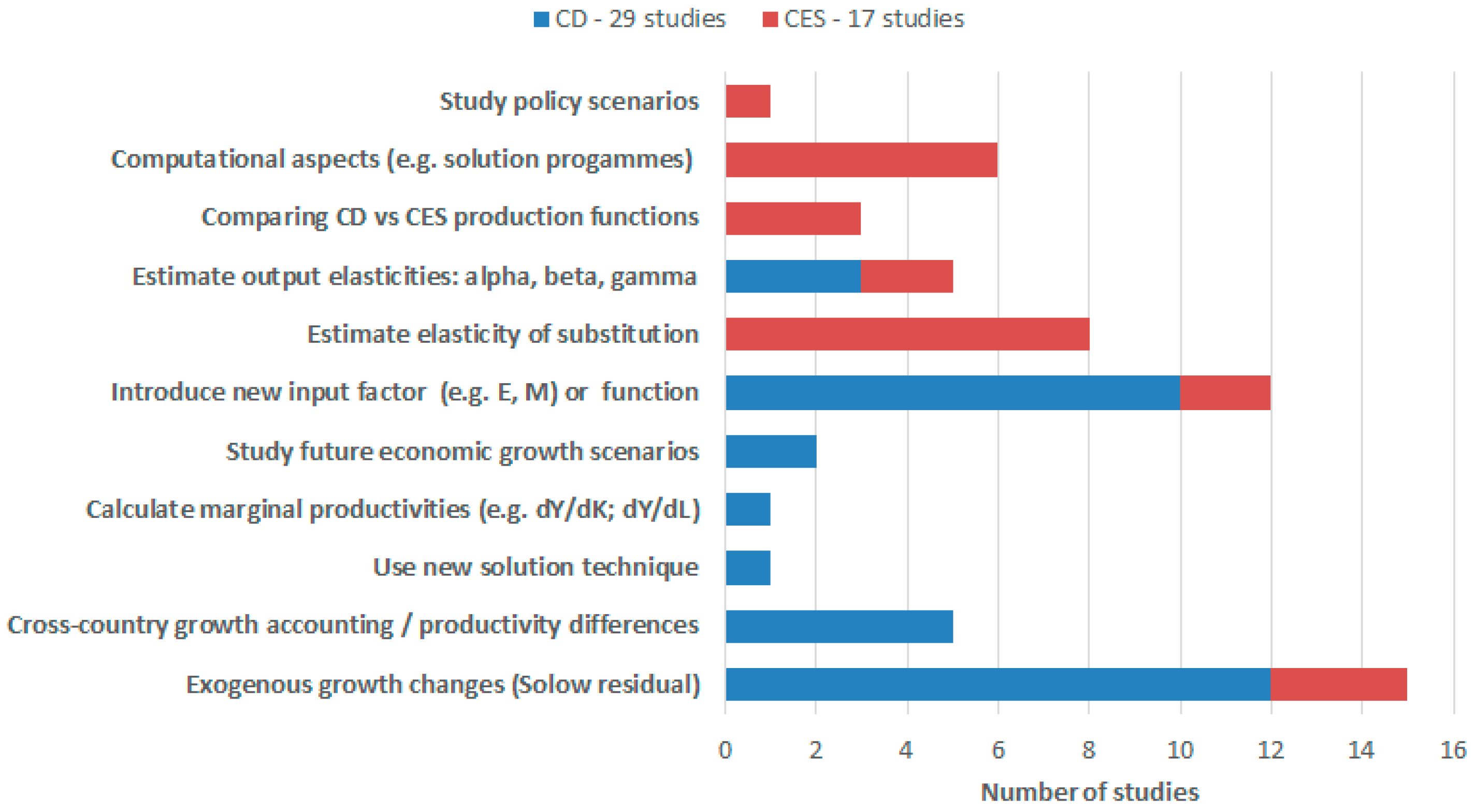
We now briefly review common applications of C-D and CES aggregate production functions. The inclusion of the C-D function (in addition to the CES function) is intended to show the changing focus of application as the C-D function is increasingly replaced by the CES function. We start with a sample survey, and then move to a wider literature search.

2.1. Sample Survey

We studied a small sample of the Google-Scholar results in Figure 1, seeking to identify similarities and differences in applications. Whilst Google-Scholar returned results for all production function types (i.e., firm level to sectoral to economy-wide scales), it nevertheless provides a guide as to the context and application of production function studies. We reviewed 46 studies [1,4,6,15,16,22,23,25,46,49,50,51,52,53,54,55,56,57,58,59,60,61,62,63,64,65,66,67,68,69,70,71,72,73,74,75,76,77,78,79,80,81,82,83,84,85], with 29 C-D and 17 CES studies, in proportion with their number in the total returned results. To make the best of the tiny, biased sample (0.1% of 40,000 Google-Scholar references obtained for Figure 1), we selected studies based on three criteria. First, studies were selected based on Google Scholar’s “highest returned relevance”—which is a metric based on the publication’s full text, the source publication and author, and the number of scholarly citations. Secondly, this is then filtered to only include empirical studies at an aggregate (sector or economy-wide) scale. Thirdly, we selected studies in proportion with the number of CES and C-D studies in each decade in Figure 1—which was intended to get some sense of the change in direction/focus of the studies, and to give insights into the transition (in popularity) from C-D to CES functions.
Figure 2 shows a histogram of the different purposes driving the C-D and CES sample studies. For C-D studies, the most common purpose was analysing historical changes in exogenous component of economic output (Solow residual), and studying new factors of production in addition to capital and labour. As the CES studies allow non-unity elasticities of substitution, and are weighted (in number) towards more recent studies, this helps explain their focus on elasticities of substitution and computational methods (e.g., use of new parameter estimation algorithm).
The output measure was almost exclusively GDP, with the key differentiator being whether it was GDP in constant prices (30 No.) or GDP per worker (14 No.).
Figure 3 shows the wide variation for choice of factors of production. For the conventional factors of production of capital and labour, capital stock and number of workers were the most common metrics. Energy was the most popular additional factor of production, appearing first in the post oil-crises 1970s [22,23], and reappearing in our sample in the 1990s [1,25,57,64,79,83]. It is interesting to see in our sample—but unclear why—the C-D studies favoured price-adjusted energy (e.g., values in £), versus the CES studies which used thermal energy content of primary or final energy (e.g., values in Joules).

2.2. Wider Literature Search

Including energy as a factor of production starts from the idea that variables in addition to labour and capital—such as energy [22,23,70], materials [46,86] or money balance [52,55]—help explain economic output. As far back as 1974, Binswanger and Ledergerber [87] suggested that “the decisive mistake of traditional economics is the neglect of energy as a factor of production”. However, including energy as a factor of production remains controversial. One argument is that energy is not an independent, primary input, but instead as an intermediate quantity made by labour and capital is thereby redundant (see Dales’ Biophysical GEMBA model as an example reflecting this argument [88,89]). To counter, the same argument could be applied to capital (i.e., you cannot make capital without labour), and authors including Stern [90] advocate energy as an independent factor of production. Some authors go further: Kümmel [91] suggests energy is the only factor of production, with capital and labour therefore intermediate products (of energy). Denison [20] suggests a second argument: that energy’s low “cost-share” (typically below 10% of GDP [92,93]) means it can only make a correspondingly small contribution to economic growth. However, authors including Stresing et al. [94] have sought to debunk this argument, whilst Aucott and Hall [95] show how—despite its low “cost-share”—small variations in energy prices have significant impacts on economic output.
Aggregate production functions themselves are not without criticism. Indeed Mishra ([96], p. 20) suggests they are “the most turbulent area of research in the economics of production”. Criticism occurs on three main fronts. First is the accounting identity critique [97,98], which infers the C-D function can be derived from an income accounting identity: output equals wages plus profits. This is held to explain the excellent historical fits, with observed correlation coefficients (R2) commonly above 0.99 [15,16]. Later, Felipe and McCombie [99] extended the accounting identity argument to include the CES function. Second, are concerns about measuring capital: Robinson [100] and Fisher [101] were among a group involved in the 1950s–1970s “Cambridge-controversy”, who suggested aggregate capital could not be measured, thereby invalidating the use of aggregate production functions. Third are empirical concerns, since factors of production typically explain only a minority of economic growth, leading Solow ([3], p. 312) to remark “it takes something more than the usual ‘willing suspension of disbelief’ to talk seriously of the aggregate production function”.
Despite on-going critiques [102,103,104], the practical reality is that: (1) “economists have continued using the aggregate production function in both theoretical and applied works” ([98], p. 262); and (2) that energy is increasingly used as a factor of production by a wide set of studies beyond academia, including government agencies [8,68,82,105] and central banks [67,106,107,108,109]. Several reasons may explain this. First, is the “pull” from energy-related questions including macroeconomic energy rebound [110,111], the contribution of energy to reducing exogenous growth [112], and climate and economic implications of energy transitions [5,113]. Second, since the elasticity of substitution (σ) is an important parameter in economics [114,115], significant effort in capital–labour–energy CES empirical analysis is directed to estimate values of σ [1,33,46,83]. Third, the comparison between CES and C-D functions is an important study focus—whether for cross country comparisons [6], specific countries [81], sectors [105] or business cycles [84]. Fourth, general equilibrium models are an important application of the empirical CES study results, as highlighted by van der Werf [25], and are widely used to assess the impact of policy [116,117]. CGE models are the most popular, and are commonly CES-based [30,48,117,118] since this allows non-unity elasticity of substitution values, but may also include C-D modules [47,119,120]. Dynamic Stochastic General Equilibrium (DSGE) models are less common, but also use CES production functions [84,121].
Overall, capital–labour–energy CES aggregate production functions have emerged into widespread usage, serving as a good compromise between complexity (of the analysis) and flexibility (i.e., wider range of available parameters). For example, Stern and Kander ([5], p. 58) noted their choice of CES over translog production function was because “we decided that it was better to model some of the main features more reliably or believably [in a CES function] than to attempt to model many features of the data less reliably [in a translog function]”.

3. Empirical CES Model—Specification

3.1. Economic Output (Y)

Three broad classes of economic output (the dependent variable, Y) exist: Gross Domestic Product (GDP), Gross Value Added (GVA)—also called Net Output, which is equal to GDP minus subsidies and taxes, and Gross Output (GO)—equal to GDP plus intermediate inputs. (Note also the valuable in-depth work on this by Hulten [122] and Cobbold [123]). In our case, it seems initially straightforward (at an economy-wide level) to select economic output as GDP, since this the most common metric nationally reported, and has been widely adopted in mainstream growth accounting [69,124], which adopts labour and capital as the two production inputs. However, when energy is added to the production function, things change, as this “intermediate” input is used by industry to produce final “products” for end consumers. Ideally, the output measure should be selected “so that the total value of output is equal to the total value of inputs” ([5], p. 59). Those working with capital–labour–energy–materials (KLEM) productivity databases, such as O’Mahony and Timmer [125], use gross output as the economic output measure. In the capital–labour–energy case, lacking materials, a measure somewhere between GVA and gross output seems logical, and this is indeed the path taken by Kander and Stern [126] and Van der Werf [25], who adopt a modified “gross output” measure as GVA plus the value (cost) of energy. It is revealing though that this is not a common approach, as empirical K-L-E CES studies adopt a wide range of output metrics, as shown in Table 1:
A second important issue is whether to specify output in (more common) constant prices [15,69,70,74] or Purchasing Power Parity (PPP) prices [25,82]. Since PPP places a higher weight on GDP in non-OECD countries—one $US Dollar in China buys more goods than in the US—PPP may be useful in cross-country studies [129,130] by providing a more level playing field for comparisons.

3.2. Factors of Production (K, L, and E)

3.2.1. Unadjusted (Basic) Factors

Studies commonly adopt capital stock (K), labour (L) and primary energy (E), which we can consider as unadjusted (or basic) factors of production, i.e., they are measured without taking into account qualitative differences. Capital stock (the estimated market value, in currency units, of assets involved in production) is most commonly derived via the Perpetual Inventory Method (PIM), where an assumed initial capital stock valuation changes each year via additions (new stock) minus subtractions. Gross capital stock (GCS) defines subtractions as retirements of existing assets; whilst Net Capital Stock (NCS) is equal to GCS less depreciation of existing assets. With NCS and GCS data published by statistical agencies [131,132], CES studies have adopted both NCS [74,133] and GCS [22,25] datasets. For labour, three options for unadjusted values of workforce labour exist, listed here in descending accuracy as a measure of labour input: work-hours [22,73], numbers of workers [33,105], or population (for economy-wide studies only) [85]. Unadjusted energy—typically given in energy units as terajoules (TJ) or million tonnes of oil equivalent (mtoe)—can be based on primary energy values or final (purchased) energy. Economy-wide studies most commonly use primary energy [33], whilst sector-level studies only use final energy [1,25,46] since primary energy values are not reported at that level.
Overall, these unadjusted variables remain very popular for empirical production function analysis, due to the availability of national and international time series across countries and sectors [134,135,136,137].

3.2.2. Quality-Adjusted Factors

Quality-adjusted values for capital (K*), labour (L*) and energy (E*) seek to better represent the productive effect of the basic factors of production (K, L, and E) on economic output (Y). Since quality-adjusted factors of production typically grow faster than unadjusted values [35,133], in such cases their use at an economy-wide scale assigns more of the increase in economic output to the growth in factors of production, and less to exogenous technical change (i.e., Solow residual).
Quality adjustment of capital can be achieved by estimating “capital services”, defined as “a flow of productive services from the cumulative stock of past investments”([138], p. 7). Consider a machine in a factory: its capital service can be measured by multiplying the price of the goods by the amount of goods produced by the machine in each year. As national-level time-series of capital services emerge [139], their use and application in empirical CES studies is increasing [69,133]. A less common alternative is capital utilisation, which estimates how productively capital equipment is used following economic cycles (i.e., less in recessions, more at other times), as shown in Paquet and Robidoux’s Canadian study [140].
Quality adjustment of labour multiplies (unadjusted) work-hours by a quality index—commonly of worker schooling or skills. As international datasets of such quality metrics—such as Barro and Lee [141]—have become more available, quality-adjusted labour appears more widely used in CES studies [58,65,72,142].
Quality-adjusting energy seeks to capture “the relative economic usefulness of different fuels and electricity” ([143], p. 302). This can be done on either a physical or economic basis. An example physical approach can consider the amount of exergy (available energy) of the energy carrier nearer the end of the energy conversion stage as useful work [144], when it is lost in exchange for energy services. Regarding economic approaches, Cleveland et al. [143] suggest higher fuel prices are indicators of higher quality, whilst Stern ([145], p. 1474) introduces a substitution method whereby quality can be measured by “how much of one fuel is required to replace another”. Weighting can range from simple aggregation to Divisia indices. Including quality-adjusted energy in empirical aggregate production function studies are rare: Ayres and Warr used the physical approach by including useful work data in economy-wide C-D and LINEX functions [144,146], whilst Stern and Kander [5] provide an economic-based CES example, using a Divisia weighted price based method for energy quality.
Despite the apparent merits of quality adjustment [63], caution is needed. For capital services, Inklaar [147] raises concerns about the accuracy of the methodology, such that the Penn World Tables (PWT) retains capital stock for its capital data [124]. For energy, economic approaches can be problematic—for example energy price data varies with sector and end use and may be distorted by taxes and subsidy effects, whilst simple price weighting is biased as it assumes no restrictions on substitutability between energy inputs [24]. As for physical approaches to energy quality, few national datasets exist of thermodynamic “useful energy”, leaving researchers to time-consumingly construct their own datasets [148,149]. The result is that most CES empirical studies continue to use unadjusted energy, i.e., primary or final energy datasets [25,83].
Interestingly, empirical studies involving only capital and labour expend significant effort to quality adjust at least one variable [57,85,108,150], but those introducing energy as a third variable typically use unadjusted values for capital and labour [1,25,79,151]. This seems surprising, but perhaps reflects the significant effort required to develop or obtain time-series of quality-adjusted variables.

3.3. Nesting and Elasticity of Substitution

Nesting, and elasticity of substitution, are interlinked aspects of CES function specification: the choice in one affects the other—so they are presented and discussed together in this section.

3.3.1. Nesting

Once the CES function has more than two factors of production, the issue of whether—and how—to nest them, arises. To see why, let us view the non-nested CES function introduced by McFadden [152], and used by Edenhofer et al. [153]. It is given in Equation (9), using the notation of nested Equation (6):
Y t = θ   e λ t [ K t ρ + L t ρ + E t ρ ] ν ρ
This formulation assumes all factors of production are equal substitutes (σ = 1/(1 − ρ), which is highly restrictive and as Broadstock et al. ([154], p. 55) note, this “appears unlikely in practice and also excludes the possibility of complementarity”. As a result, various authors [25,26,44] report this structure is rarely used, with instead CES studies preferring to “nest” the factors of production, which is more flexible by allowing different elasticities of substitution to exist between production factors. A nested three factor format typically has two factors of production placed within an “inner” nest and one in an “outer” nest. Such a nest is shown in Figure 4, which portrays the KL(E) nesting structure of Equation (6), given earlier, where capital–labour is in the inner nest, and energy sits in the outer nest.
Van der Werf [25] reviewed numerous capital–labour–energy (KLE) and capital–labour–energy–materials (KLEM) production functions used in climate-based models. He found whilst most studies analysed a single, KL(E) nest—a view supported by Zha and Zhou [26]—there was also considerable variation in nesting structure. This presents two routes forward for analysts. The first is to constrain the empirical analysis to a single nesting structure, based on a-priori theoretical or other considerations. For example, Saunders [31] suggests the KL(E) nesting is the nesting structure that permits the fullest range of energy rebound (Re): from hyperconservation (Re < 0) to backfire (Re > 1). The second, less common approach, is to separately estimate and report all three types of nesting [1,25,33,79]—though care is needed in interpretation, since certain solution aspects (such as elasticity of substitution) will not be comparable between different nestings.

3.3.2. Elasticity of Substitution, σ

Interwoven with the issue of nesting is the elasticity of substitution, σ, which tells us the ease by which one factor of production (e.g., labour) is substitutable by another (e.g., capital). For aggregate production functions and downstream macroeconomic models, we most commonly assign sigma ( σ = 1 1 + ρ ) as the Hicks Elasticity of Substitution (HES). Taking the CES function in Equation (6), this leads to the special cases where capital and labour have zero substitutability (i.e., are complements) in a Leontief function ( σ = 0 ); some substitutability in a C-D function ( σ = 1 ), and are perfect substitutes in a linear function ( σ = ). Chirinko and Mallick [114,155,156] highlight the importance that conventional economics places on the elasticity of substitution between capital and labour—which appears borne out by Thomas Piketty’s recent work [157] and the subsequent flurry of academic debate [158,159,160]. (However, it also reveals how orthodox economists continue with capital–labour aggregate production functions that ignore energy as a factor of production.).
With multiple factors of production several key issues appear regarding the elasticity of substitution. The first relates to the confusion and mis-use stemming from multiple definitions of elasticity of substitution in common use—Stern [10] for example reviews ten different elasticities, including the Allen Elasticity of Substitution (AES), Cross-price elasticity (CPE), and Morishima Elasticity of Substitution (MES). Whilst different elasticities may be appropriate for different purposes—for example Klump and de La Grandville [161] recommended the use of MESs when studying economic growth, whereas Sancho employs HESs for CGE model calibration [118]—the multiple definitions are confusing. The choice of elasticity matters, since whilst some elasticities (e.g., AES = HES) are equal for two-input functions [162], they are not in our three factor (K, L, and E) CES function case. This creates the situation where downstream mis-use of elasticities occurs. For example, Sorrell is critical of the use of non-HES elasticities for CGE modelling, since “estimates of the [more commonly estimated] AES, CPE or MES between two inputs provide little guidance in choosing the appropriate values of the HES between those inputs that are required for the nested CES functions used in CGE models.” ([163], p. 2863). Meanwhile, Van der Werf [25] (p. 2965), argues that even if HES values are selected from the literature, they are likely to be incorrect since “in most applied dynamic climate policy models, neither the production structure nor the accompanying elasticities of substitution have an empirical basis.”
The second issue is the impact of nesting structure on the elasticity of substitution. Sato’s [164] two-level nest CES function in Equation (6) permits separate values for inner-nest (K-L) elasticity σ 1 = σ K L and outer-nest (KL-E) elasticity σ = σ K L , E ,—which he tells us can be used to justify nesting choice:
Introspection tells us that the [inner-nest] elasticities of substitution should be substantially higher than the [outer-nest] elasticity. After all, we justify the aggregation by the fact that aggregated factors are similar in techno-economic characteristics. One of such similarities is obviously the ease of substitution.
[164] (p. 203)
Sorrell [163] (p. 2863) picks up the implication of this important point, suggesting “estimates of substitution elasticities are likely to be biased if separability is assumed where not supported by the data”. This means that the choice of nesting structure matters (e.g., KL(E) versus EK(L)), and amounts to imposing separability on the factors of production—since they are forced into nesting structures that may not match the data. Van der Werf [25] continues, illustrating how the estimated elasticity between two factors of production (e.g., K-L) vary significantly depending on the nesting structure.
Third, is that, as Sato [164] showed, in a two-level CES function only one of the two partial elasticities is actually constant over time, except in restrictive cases. An example is the constrained CES function based on Hogan and Manne [165], where the capital–labour inner-nest is assumed as a Cobb–Douglas function ( σ = 1), as given in Equation (10). Saunders [31] adopts this approach, as do some CGE models [166,167]. However, by setting (pre-analysis) elasticity of substitution values for the inner nest, this constrains the available values for all parameters to be estimated, including the outer nest elasticity of substitution.
Y t = θ   e λ t [ δ ( K t α L t ( 1 α ) ) ρ + ( 1 δ ) E t ρ ] 1 ρ
All of this matters, since estimated parameters—such the elasticity of substitution in empirical CES studies [25,26,46,163]—can have a large influence on macroeconomic model results. For example, with a KL(E) nest, Jacoby et al. [168] found changes to the elasticity of substitution was the main driver of differences in their CGE model results, whilst in relation to energy rebound, Saunders, who first suggested the sensitivity (and thus importance) of elasticity of substitution to energy rebound [169] subsequently found empirical support for this assertion [110].

3.4. Other CES Function Parameters

3.4.1. Productivity/Technical Change Coefficients

The exogenous part of economic output (as captured by the term e λ t in Equation (6) can also be stated as Hicks-neutral technical progress [170], with λ a measure of its rate of change. This means productivity changes are neutral—rather than biased—across factors of production. Whilst many studies employ this assumption [79,83], it is restrictive since it assumes the productivity of labour, energy and capital all increase at the same rate, which may simply not be true.
To overcome this restraint, separate productivity coefficients ( τ K , τ L , and τ E ) can be introduced (omitting the time dependant suffix from τ for ease of viewing) as first shown in a 3-factor CES specification by Saunders [169], and estimated for each factor of production. In our case, this modifies Equation (6) such that τ K , τ L and τ E replace the (now redundant) term e λ t , as shown in Equation (11). The productivity coefficients represent technological changes of each production factor while leaving the productivity of the others unchanged. Sorrell [163] describes this as giving the separate coefficients’ ability to assign bias in technical change to specific production factors. Note if τ K = τ L = τ E , Equation (11) returns to the Hicks-neutral Equation (6).
Y t = θ   [ δ 1 [ ( δ   τ K K t ρ 1 + ( 1 δ ) τ L L t ρ 1 ] ρ / ρ 1 + ( 1 δ 1 ) τ E E t ρ ] ν ρ
In a capital–labour–energy CES production function context, van der Werf [25] and Dissou et al. [1] provide examples of this method, estimating directly the technical change parameters assigned to the factors of production. Papagerogiou et al. [171] extend this approach, by splitting fossil fuel and renewables adopting separate technical productivity coefficients.
However, a central caveat is that the factor-augmenting technical change parameters are likely to overlap with the use of quality-adjusted inputs given earlier, for example “effective labour” (as depicted by τ L L) is closely related to quality-adjusted labour (human capital index × labour).

3.4.2. Returns to Scale, (ν)

Empirical CES studies almost exclusively assume unity returns-to-scale (ν = 1), which is an important economic assumption, and matches the popular CES specification set by Arrow et al. [12]. This restrictive assumption is tested by Layson [172], who finds the generalized CES function (where ν is unconstrained) allows an “explosive” case (where ν and σ are >1). Szeto [82]—who estimated ν = 1.09, and Duffy and Papageorgiou [6]—who estimated ν = 0.97–1.00, provide rare generalized CES function examples. Curiously, both these economy-wide studies were then returned to ν = 1, since as Szeto [82] (p. 7) noted “theory suggests that there are constant returns to scale in production, we will impose this restriction in the remainder of our empirical analysis”. One caveat attached to the unconstrained approach is that whilst the results will indicate how well the model supports the unity returns-to-scale assumption, the model will have fewer degrees of freedom, meaning the parameter estimates will be less precise.

3.4.3. Output Share Parameters, δ , δ 1

In the capital–labour C-D function given in Equation (1), it is a mathematical result that the partial output elasticity for capital (α) and labour (β) is equal to the respective cost-shares of aggregate output (typically around 0.3 for capital, 0.7 for labour)—under the neoclassical assumptions that firms are profit maximizing and markets are perfectly competitive. However, in the nested capital–labour–energy CES function, the output share parameters ( δ ,   δ 1 ) in Equations (6)–(8) are not equal to (and therefore cannot be set as) the time-varying output elasticities ( α K ,   α L , α E ), as shown in Equation (12)—adapted from Heun et al. [35]. (The exception is the limiting C-D case where ρ = 0).
α E = Y E Y E = 1 δ δ E ρ [ δ 1 K ρ 1 + ( 1 δ 1 ) L ρ 1 ] ρ ρ 1 + 1 δ

3.5. Normalisation

A historical complaint about aggregate production functions is that they combine different units, e.g., capital ($), labour (h), and energy (TJ), generating “production function parameters [that] have no economic interpretation” [108] (p. 7). One approach to overcome this critique is to normalise the factors of production prior to estimating the unknown parameters, since this “removes the problem that arises from the fact that labour and capital are measured in different units” ([104], p. 30). The method indexes time-series data to the base year, so y = Y t / Y 0 ; k = K t / K 0 ; l = L t / L 0 ; e = E t / E 0 ; with the resultant normalised (lower case) version of Equation (6) shown as Equation (13):
y t = θ   e λ t [ δ 1 [ ( δ   k t ρ 1 + ( 1 δ ) L t ρ 1 ] ρ / ρ 1 + ( 1 δ 1 ) e t ρ ] ν ρ
For the estimation of aggregate production functions, the introduction and use of normalised variables (y, k, l, and e) means different estimated values can be obtained for the leading coefficient (theta) and share (delta) parameters. The latter could affect economic interpretation of the results. That said, the effects of normalisation may differ for empirical studies which base their research on estimating first-order conditions rather than the overall production function.
Advocates of normalization include La Grandville, Klump, and co-authors [32,108,173], who suggest advantages including a more comparable basis to study elasticities of substitution between different studies [33,115]. That said, caveats do exist: for example Temple [34] comments on the misuse of normalization for certain applications. Returning to capital–labour–energy CES empirical studies, normalization has yet to make significant inroads—Shen and Whalley [33] and Heun et al. [35] provide rare examples—but this may change as the use and publication of indexed aggregate datasets such as those of Jorgenson [174] should aid their dissemination and usage in growth accounting.

4. Empirical CES Model—Parameter Estimation

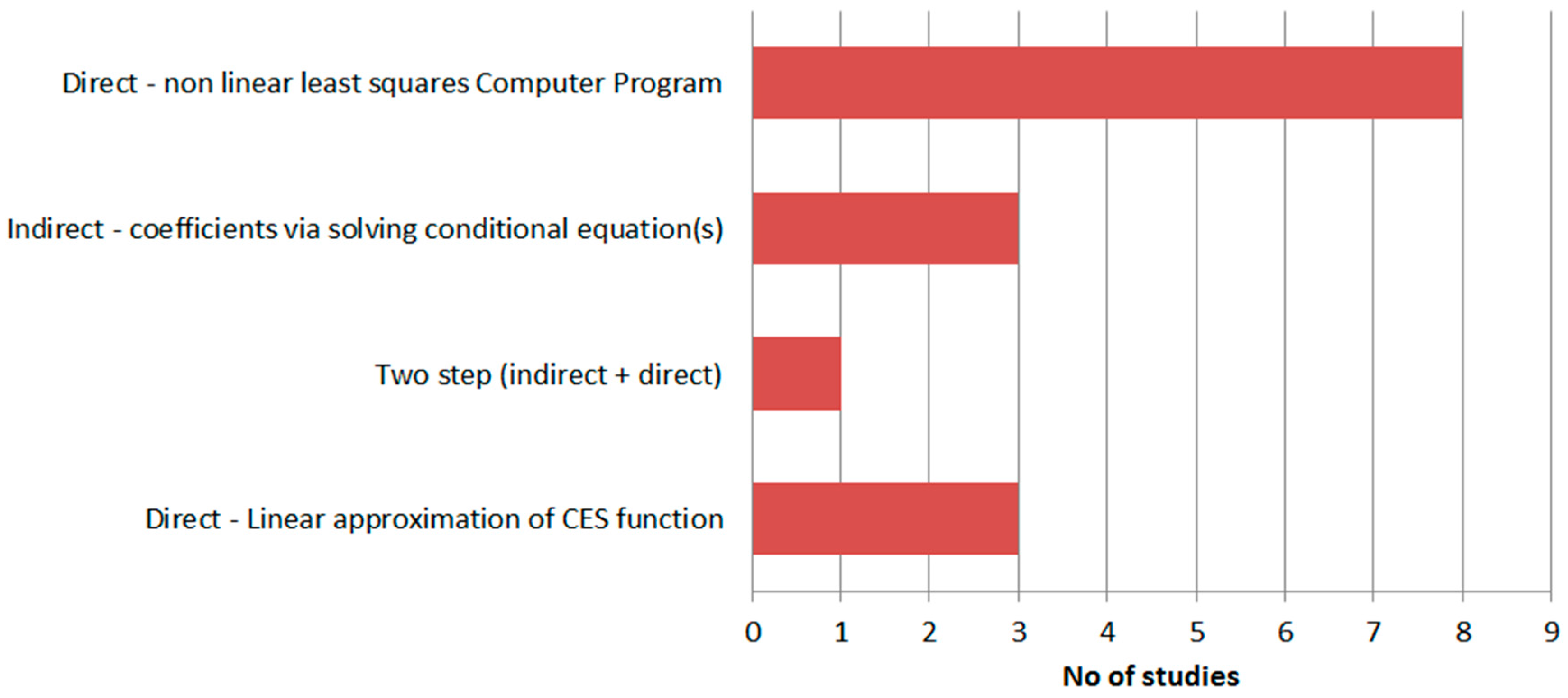
4.1. Estimation Methods

The C-D function in Equation (5) is typically estimated as a linear equation by ordinary least squares (OLS), after first taking logarithms. This simple, linear solution method is one reason for its enduring popularity. However, the CES function in Equation (6) cannot be transformed in the same simple manner to a linear equation without approximation, and so numerous other techniques have been developed, as evidenced by the CES sample studies shown in Figure 5.
The most popular technique in the sample—used by over half the sample [1,6,46,77,78,79,82,83]—is direct non-linear estimation of the aggregate function. Though complex, its popularity appears to be increasing, which may be due to the increased availability of econometric guidance [175], off-the-shelf programmes [30], and advances in computing power. A common method is a grid based search over relevant parameter ranges, such as that set out by Henningsen and Henningsen [30,176], and used by Heun et al. [35]. Though non-linear techniques appear attractive to solve the inherently non-linear CES function, and have been found to perform better than linear alternatives [46]—care needs to be taken: for example Papageorgiou et al. [171] (p. 26) note that “results of non-linear estimation procedures maybe sensitive to the choice of starting values of the estimation parameters”.
A second method indirectly estimates the parameters, since the solution to the non-linear function is not directly estimated. Instead, three linear simultaneous equations—one for each factor of production—are derived, based on applying the important first-order economic assumption of equality between factor prices and marginal products to the CES function—also known as Shephard’s Lemma. This method is a common approach where the sole parameter of interest is the elasticity of substitution (σ), as Van der Werf [25] and Dissou et al. [1] show. However, systems estimation carries with it additional risks, for example misspecification in one equation can have deleterious consequences for estimates in other equations in the system.
Third, is a hybrid indirect-direct method, based on Nerlove’s 1967 two-step process [177]. Bonga Bonga [81] provides a rare, recent example, which in the first step estimates the elasticity of substitution (σ) and distribution parameter (δ), based on the estimated ratio of marginal productivities under perfect competition, and then in the second step inserts σ and δ back into the CES equation, reducing it to a linear equation which is then directly estimated.
A fourth method used is direct linear approximation, based on Kmenta’s 1967 simplification of the non-linear CES equation [178]. However, since the Kmenta approximation cannot be used to linearise CES production functions with more than two factors of production [176], it is found only in our samples for two factor (capital–labour) studies [6,74,85], and is therefore not a valid estimation technique for the energy-extended (capital–labour–energy) CES function.
Outside of the sample CES studies, Klump et al. [108] raise an additional, “system approach” method, which involves the non-linear solution of a “system” comprising the aggregate production function and linear first-order conditions. Two other estimation points are notable. The first relates to the “endogeneity problem” raised by Mundlak [179]—where an explanatory variable is correlated with the error term in a regression. Malleck [156] is amongst those who used Instrument Variables (IV) as a way around this issue. Second is that the production function is a long-run equilibrium concept, meaning as Chirinko [114] (p. 671) notes, there is a “fundamental tension between the short-run data that are available and the long-run parameter that is required”. Cointegration [180] and filtering techniques [181] offer potential routes forward.

4.2. Statistical Reporting

Statistical techniques and reporting provides important context to the empirical results. Three key aspects are considered here. The first are the common statistical tests on the fitted function and its econometrically estimated coefficients. From the sample, the majority report goodness-of-fit via the coefficient of determination (R2) [74,75,78,83] and the Durbin–Watson (D-W) value—testing for autocorrelation of the residuals of the regression [25,73,77,83]. (However, we also note that not all econometric techniques can generate the same statistics. For example, R2 is not applicable with Seemingly Unrelated Regressions). The overall F-test—giving the statistical significance of the overall relationship—was less commonly reported [75,77,81]. Within our sample, only Easterly and Fischer [78] and Duffy and Papageorgiou [6] reported tests for heteroskedasticity in the error term (i.e., the fitted residual).
The second important aspect is the reporting of p-values on the statistical significance of individual coefficients, which is also common [6,25,77,82], but should be used (and viewed) with caution. This is because p-values are a measure of the evidence against a null hypothesis, with small p-values indicate overwhelming evidence against the null. Statistical fitting software typically assumes the null hypotheses that fitted parameters are zero, which may not be meaningful for some parameters of the CES production function, for example the share parameter, δ. In short, analysts should be very careful that reported p-values accord with the purposes of a study.
A third aspect relates to the reporting of standard errors, which adds important information about the precision with which parameters are estimated. For example, in a study examining the substitutability of energy for the capital/labour composite in a (KL)E nesting structure (Equation (4)), the value of sigma is central. If sigma is reported as 0.5 with standard error of 0.3, it will be hard to claim whether KL and E are substitutes or complements. If, instead, sigma is found to be 0.95 with standard error 0.02, it could reasonably be claimed that KL and E are substitutable. Bootstrap resampling can also be used to gain valuable insights on the precision of the estimated parameter values. This may be particularly relevant for study of parameters estimated close to economically-meaningful boundaries (e.g., delta = 0.96), which are unlikely to have symmetric distributions. Whilst none of the sample studies used this technique, it is entering the wider growth accounting literature [109,171,182], and can be applied to empirical CES analyses, as shown by Heun et al. [35].
Overall, whilst statistical reporting can strengthen the empirical results and provide better context for comparison of results between studies, it seems an aspect of the estimation process that is under-reported at present.

5. Recommendations

From the collated aspects in Section 3, we provide a summary of CES specification recommendations in Table 2.
Two key aspects of CES specification are worthy of further discussion here. First is the linked issue of output measure and normalization. We saw earlier the variation in Table 1 relating to choice of output measure in empirical energy-extended CES studies. This was a surprising finding, and one we would expect perhaps to change in future, if a consensus emerges—e.g., towards a “modified” gross output (GVA + energy cost). Allied to this is the effect (and thus importance) of normalization. If absolute measures of economic output (Y) are used when fitting the CES aggregate production function, a change from GDP to GVA or gross output will affect parameter estimates if GVA or gross output are different from GDP, as they are likely to be. If indexed (normalized) measures of economic output (Y) are used when fitting the CES aggregate production function, a change from GDP to GVA or gross output will affect parameter estimates only if the indexed value of GVA or gross output is different from the indexed value of GDP. i.e., estimates of fitted parameters will not change if GVA or gross output is different from GDP by a constant multiplicative factor only. Second—and related to the first—is the issue of quality-adjusted inputs. Whilst desirable, two caveats can be attached: (1) that quality-adjusting inputs can bring a direct conflict/duplication with technical change parameters, τ; and (2) there are different methods of quality-adjusting each input (capital, labour and energy). In sum, this means great care is required to construct the inputs properly, and to align them to the chosen output measure.
Moving to CES estimation, two recommendations from Section 4 are made. First is the advocation—with caveats—for the common use of off-the-shelf non-linear coding to solve the aggregate function such as Henningsen and Henningsen [30]. The caveat is that caution is required: there are issues such as near boundary solutions and multiple solutions which require attention—see Heun et al. [35]. Second is the desire for the deepening of statistical reporting via: (1) reporting all nesting structure results; and (2) greater reporting of the estimated precision of parameter values, such as through bootstrap resampling.
Finally, looking forward, to ultimately provide better inputs to energy policy, effort in two key areas is required. First, more detailed research by the energy economics community is required specifically to investigate the impacts of modelling choices (e.g., normalization, or quality adjusting inputs) on estimated parameter results. This will help identify which of the CES modelling choices have the most significant impacts on results. The empirical “sister” to this current paper by Heun et al. [35] is an intended next step in this direction. By improving understanding of modelling parameters, this will also better inform users of the analytical results—e.g., CGE modellers and policy-makers—as to the robustness and sensitivity of assumed parameters. Second, empirical CES studies currently exhibit great variation in the type of results reported. Developing a consistent approach to reporting would add interpretative value to the study itself, and enable improved inter-study comparisons. For example, studies could consistently report results showing the effect of: (1) new datasets (e.g., new quality-adjusted verses incumbent non-adjusted variable); (2) different nesting structures; and (3) the application of broader statistical techniques (e.g., standard errors and bootstrapping).

Acknowledgments

We gratefully acknowledge the support of Engineering and Physical Sciences Research Council (EPSRC) and Arup for contributing to the PhD CASE (Collaborative Award in Science and Engineering) scholarship of Paul Brockway. Paul Brockway’s time was also funded in the later stages of this work as part of the research programme of the UK Energy Research Centre (UKERC), supported by the UK Research Councils under EPSRC award EP/L024756/1. João Santos was financially supported by FCT/MCTES (PIDDAC) through project UID/EEA/50009/2013. The support of the Economic and Social Research Council (ESRC) is also gratefully acknowledged. The work contributes to the programme of the ESRC Centre for Climate Change Economics and Policy. We also gratefully acknowledge comments and inputs from Timothy Foxon, Randy Prium, Marco Sakai, Steve Sorrell, and Julia Steinberger during the development of the paper. Finally, we would like to thank the three anonymous reviewers whose comments have strengthened the paper.

Author Contributions

Matthew K. Heun, Paul E. Brockway conceived this landscape paper at the 2014 International Exergy Economics Workshop in Leeds, England, 19–20 May. Paul E. Brockway led the narrative framing for the paper and coordinated its writing. All co-authors provided substantial inputs to writing and significant comments on numerous drafts.

Conflicts of Interest

The authors declare no conflict of interest.

References

  1. Dissou, Y.; Karnizova, L.; Sun, Q. Industry-level Econometric Estimates of Energy-capital-labour Substitution with a Nested CES Production Function. Altlantic Econ. J. 2012, 43, 107–121. [Google Scholar] [CrossRef]
  2. Smyth, R.; Kumar, P.; Shi, H. Substitution between energy and classical factor inputs in the Chinese steel sector. Appl. Energy 2011, 88, 361–367. [Google Scholar] [CrossRef]
  3. Solow, R.M. Technical Change and the Aggregate Production Function. Rev. Econ. Stat. 1957, 39, 312–320. [Google Scholar] [CrossRef]
  4. Nelson, R.R. Aggregate Production Functions and Medium-Range Growth Projections. Am. Econ. Rev. 1964, 54, 575–606. [Google Scholar]
  5. Kander, A.; Stern, D.I. Economic growth and the transition from traditional to modern energy in Sweden. Energy Econ. 2014, 46, 56–65. [Google Scholar] [CrossRef]
  6. Duffy, J.; Papageorgiou, C. A Cross-Country Empirical Investigation of the Aggregate Production Function Specification. J. Econ. Growth 2000, 5, 87–120. [Google Scholar] [CrossRef]
  7. Felipe, J.; Adams, F.G. A Theory of Production: The estimation of the Cobb-Douglas Function: A Retrospective View. East. Econ. J. 2005, 31, 427–445. [Google Scholar]
  8. Miller, E. An Assessment of CES and Cobb-Douglas Production Functions; US Congressional Budget Office Working Paper 2008–05; US Congressional Budget Office: Washington, DC, USA, 2008.
  9. Cobb, C.; Douglas, P. A theory of production. Am. Econ. Rev. 1928, 18, 139–165. [Google Scholar]
  10. Stern, D.I. Elasticities of substitution and complementarity. J. Prod. Anal. 2011, 36, 79–89. [Google Scholar] [CrossRef] [Green Version]
  11. Solow, R. A Contribution to the Theory of Economic Growth. Q. J. Econ. 1956, 70, 65–94. [Google Scholar] [CrossRef]
  12. Arrow, K.; Chenery, H.; Minhas, C.; Solow, R. Capital-Labor Substitution and Economic Efficiency. Rev. Econ. Stat. 1961, 43, 225–250. [Google Scholar] [CrossRef]
  13. Crafts, N. Solow and Growth Accounting: A Perspective from Quantitative Economics History. In Proceedings of the 20th Annual History of Political Economy Conference: Robert Solow and the Development of Growth, Urham, NC, USA, 25–27 April 2008.
  14. Denison, E.F. The Sources of Economic Growth in the United States and the Alternatives Before US; Supplementary Paper No 13; Committee for Economic Development: New York, NY, USA, 1962. [Google Scholar]
  15. Desai, P. Total factor productivity in postwar Soviet industry and its branches. J. Comp. Econ. 1985, 9, 1–23. [Google Scholar] [CrossRef]
  16. Chow, G.C.; Li, K.-W. China’s Economic Growth: 1952–2010. Econ. Dev. Cult. Chang. 2002, 51, 247–256. [Google Scholar] [CrossRef]
  17. Abramovitz, M. Resource and Output Trends in the United States since 1870; National Bureau of Economic Research: Cambridge, MA, USA, 1956; Volume 46, pp. 5–23. [Google Scholar]
  18. Hulten, C.R. Total Factor Productivity: A Short Biography. In New Developments in Productivity Analysis; Hulten, C.R., Dean, E.R., Harper, M.J., Eds.; University of Chicago Press: Chicago, IL, USA, 2001; pp. 1–55. [Google Scholar]
  19. Jorgenson, D.W.; Griliches, Z. The explanation of productivity change. Rev. Econ. Stud. 1967, 34, 249–283. [Google Scholar] [CrossRef]
  20. Denison, E.F. Accounting for Slower Economic Growth: The United States in the 1970’s; Brookings Institution Press: Washington, DC, USA, 1979. [Google Scholar]
  21. Hulten, C.R. Growth Accounting. National Bureau of Economic Research Working Paper 15341. 2009. Available online: http://www.nber.org/papers/w15341 (accessed on 8 February 2017).
  22. Rasch, R.H.; Tatom, J.A. Energy Resources and Potential GNP; Federal Reserve Bank of St Louis Review June 1977; Federal Reserve Bank: St. Louis, MO, USA, 1977; pp. 10–24. [Google Scholar]
  23. Renshaw, E.F. Energy efficiency and the slump in labour productivity in the USA. Energy Econ. 1981, 3, 36–42. [Google Scholar] [CrossRef]
  24. Berndt, E.R.; Wood, D.O. Technology, Prices and Derived Demand for Energy. Rev. Econ. Stud. Stat. 1975, 57, 259–268. [Google Scholar] [CrossRef]
  25. Van der Werf, E. Production functions for climate policy modeling: An empirical analysis. Energy Econ. 2008, 30, 2964–2979. [Google Scholar] [CrossRef]
  26. Zha, D.; Zhou, D. The elasticity of substitution and the way of nesting CES production function with emphasis on energy input. Appl. Energy 2014, 130, 793–798. [Google Scholar] [CrossRef]
  27. Stern, D.I. Energy and economic growth in the USA: A multivariate approach. Energy Econ. 1993, 15, 137–150. [Google Scholar] [CrossRef]
  28. Bruns, S.B.; Gross, C.; Stern, D.I. Is There Really Granger Causality Between Energy Use and Output? Energy J. 2014, 35, 101–134. [Google Scholar] [CrossRef] [Green Version]
  29. Kalimeris, P.; Richardson, C.; Bithas, K. A meta-analysis investigation of the direction of the energy-GDP causal relationship: Implications for the growth-degrowth dialogue. J. Clean. Prod. 2014, 67, 1–13. [Google Scholar] [CrossRef]
  30. Henningsen, A.; Henningsen, G. Econometric Estimation of the “Constant Elasticity of Substitution” Function in R: Package micEconCES; Institute of Food and Resource Economics, University of Copenhagen—FOI Working Paper 2011/9; University of Copenhagen: Copenhagen, Denmark, 2011. [Google Scholar]
  31. Saunders, H.D. Fuel conserving (and using) production functions. Energy Econ. 2008, 30, 2184–2235. [Google Scholar] [CrossRef]
  32. Klump, R.; Preissler, H. CES Production Functions and Economic Growth. Scand. J. Econ. 2000, 102, 41–56. [Google Scholar] [CrossRef]
  33. Shen, K.; Whalley, J. Capital-Labor-Energy Substitution in Nested CES Production Functions for China; NBER Working Paper 19104; National Bureau of Economic Research: Cambridge, MA, USA, 2013. [Google Scholar]
  34. Temple, J. The calibration of CES production functions. J. Macroecon. 2012, 34, 294–303. [Google Scholar] [CrossRef]
  35. Heun, M.K.; Santos, J.; Brockway, P.E.; Pruim, R.; Domingos, T. From theory to econometrics to energy policy: Cautionary tales for policymaking using aggregate production functions. Energies 2017, in press. [Google Scholar]
  36. Pavelescu, F. Some aspects of the translog production function estimation. Romanian J. Econ. 2011, 32, 131–150. [Google Scholar]
  37. Fare, R.; Yoon, B.J. Variable Elasticity of Substitution in Urban Housing Production. J. Urban Econ. 1981, 10, 369–374. [Google Scholar] [CrossRef]
  38. Warr, B.; Ayres, R.U. Useful work and information as drivers of economic growth. Ecol. Econ. 2012, 73, 93–102. [Google Scholar] [CrossRef]
  39. Thurston, N.K.; Libby, A.M. A Production Function for Physician Services Revisited. Rev. Econ. Stat. 2002, 84, 184–191. [Google Scholar] [CrossRef]
  40. Li, T.; Rosenman, R. Estimating Hospital Costs With a Generalised Leontief Function. Health Econ. 2001, 10, 523–538. [Google Scholar] [CrossRef] [PubMed]
  41. Bentzen, J. Estimating the rebound effect in US manufacturing energy consumption. Energy Econ. 2004, 26, 123–134. [Google Scholar] [CrossRef]
  42. Saunders, H.D. Historical evidence for energy efficiency rebound in 30 US sectors and a toolkit for rebound analysts. Technol. Forecast. Soc. Chang. 2013, 80, 1317–1330. [Google Scholar] [CrossRef]
  43. Adetutu, M.O. Energy efficiency and capital-energy substitutability: Evidence from four OPEC countries. Appl. Energy 2014, 119, 363–370. [Google Scholar] [CrossRef]
  44. Lecca, P.; Swales, K.; Turner, K. An investigation of issues relating to where energy should enter the production function. Econ. Model. 2011, 28, 2832–2841. [Google Scholar] [CrossRef]
  45. Hanley, N.; McGregor, P.G.; Swales, J.K.; Turner, K. Do increases in energy efficiency improve environmental quality and sustainability? Ecol. Econ. 2009, 68, 692–709. [Google Scholar] [CrossRef]
  46. Koesler, S.; Schymura, M. Substitution Elasticities in a CES Production Framework. An Empirical Analysis on the Basis of Non-Linear Least Squares Estimations; ZEW Discussion Paper No 12-007; ZEW: Mannheim, Germany, 2012. [Google Scholar]
  47. Punt, C.; Pauw, K.; van Schoor, M.; Gilimani, B.; Rantho, L.; McDonald, S.; Chant, L.; Valente, C. Functional Forms Used in CGE Models: Modelling Production and Commodity Flows; PROVIDE Project Background Paper; TMIP FMIP: Atlanta, GA, USA, 2003. [Google Scholar]
  48. Sajadifar, S.; Arakelyan, A.; Khiabani, N. The Linear Approximation of the CES Function to parameter estimation in CGE Modeling. In Proceedings of the International Conference on Business and Economics Research (ICBER), Kuala Lumpur, Malaysia, 26–28 Novemner 2010; pp. 1–10.
  49. Feldstein, M.S. Specification of the Labour Input in the Aggregate Production Function. Rev. Econ. Stud. 1967, 34, 375–386. [Google Scholar] [CrossRef]
  50. Fisk, P.R. The Estimation of Marginal Product from a Cobb-Douglas Production Function. Econometrica 1966, 34, 162–172. [Google Scholar] [CrossRef]
  51. Hayami, Y.; Ruttan, V.W. Agricultural Productivity Differences Among Countries. Am. Econ. Rev. 1970, 60, 895–911. [Google Scholar]
  52. Prais, Z. A new look at real money balances as a variable in the production function. J. Money Credit Bank. 1975, 7, 535–543. [Google Scholar] [CrossRef]
  53. Ulveling, E.; Fletcher, L. A Cobb-Douglas Production Function with Variable Returns to Scale. Am. J. Agric. Econ. 1970, 52, 322–326. [Google Scholar] [CrossRef]
  54. Uri, N.D. The impact of technical change on the aggregate production function. Appl. Econ. 1984, 16, 555–567. [Google Scholar] [CrossRef]
  55. Khan, A.H.A.; Ahmad, M. Real Money Balances in the Production Function of a Developing Country. Rev. Econ. Stat. 1985, 67, 336–340. [Google Scholar] [CrossRef]
  56. Mankiw, N.G.; Romer, D.; Weil, D.N. A Contribution to the Empirics of Economics Growth; NBER Working Paper No 3541; National Bureau of Economic Research: Cambridge, MA, USA, 1990. [Google Scholar]
  57. Finn, M.G. Variance properties of Solow’s productivity residual and their cyclical implications. J. Econ. Dyn. Control 1995, 19, 1249–1281. [Google Scholar] [CrossRef]
  58. Dougherty, C.; Jorgenson, D.W. International Comparisons of the Sources of Economic Growth. Am. Econ. Rev. 1996, 86, 25–29. [Google Scholar]
  59. Kalirajan, K.P.; Obwona, M.B.; Zhao, S. A Decomposition of Total Factor Productivity Growth: The Case of Chinese Agricultural Growth before and after Reforms. Am. J. Agric. Econ. 1996, 78, 331–338. [Google Scholar] [CrossRef]
  60. Hall, R.E.; Jones, C.I. Why do some countries produce so much more output per worker than others? Q. J. Econ. 1999, 114, 83–116. [Google Scholar] [CrossRef]
  61. Garcia-Milà, T.; McGuire, T.J. The contribution of publicly provided inputs to states’ economies. Reg. Sci. Urban Econ. 1992, 22, 229–241. [Google Scholar] [CrossRef]
  62. Kalaitzidakis, P.; Korniotiis, G. The Solow growth model: Vector autoregression (VAR) and cross-section times-series. Appl. Econ. 2000, 32, 737–747. [Google Scholar] [CrossRef]
  63. Caselli, F. Accounting for Cross-Country Income Differences; Centre for Economic Performance CEP Discussion Paper No 667; Working Paper of Centre for Economic Performance: London, UK, 2005; pp. 1–69. [Google Scholar]
  64. Vouvaki, D.; Xepapadeas, A. Total Factor Productivity Growth when Factors of Production Generate Environmental Externalities; Munich Personal RePEc Archive—MPRA Paper No 10237; Munich Personal RePEc Archive: Munich, Germany, 2008; pp. 1–31. [Google Scholar]
  65. Autor, D.H.; Katz, L.F.; Kearney, M.S. The Polarization of the U.S. Labor Market; National Bureau of Economic Research Working Paper 11986; National Bureau of Economic Research: Cambridge, MA, USA, 2006; Available online: http://www.nber.org/papers/w11986 (accessed on 8 February 2017).
  66. Martin, W.; Mitra, D. Productivity Growth and Convergence in Agriculture versus Manufacturing. Econ. Dev. Cult. Chang. 2001, 49, 403–422. [Google Scholar] [CrossRef]
  67. Fernald, J.; Neiman, B. Growth Accounting with Misallocation: Or, Doing Less with More in Singapore; Federal Reserve Bank of San Francisco Working Paper 2010–18; Federal Reserve Bank of San Francisco: San Francisco, CA, USA, 2010; pp. 1–49. [Google Scholar]
  68. Long, K.; Franklin, M. Multi–factor productivity: Estimates for 1994–2008. Econ. Labour Mark. Rev. 2010, 4, 67–72. [Google Scholar] [CrossRef]
  69. Hájková, D.; Hurník, J. Cobb-Douglas production function: The case of a converging economy. Czech J. Econ. Financ. 2007, 57, 465–476. [Google Scholar]
  70. Yuan, C.; Liu, S.; Wu, J. Research on energy-saving effect of technological progress based on Cobb-Douglas production function. Energy Policy 2009, 37, 2842–2846. [Google Scholar] [CrossRef]
  71. The Conference Board. Projecting Global Growth; Economics Working Papers, EPWP #12-02; The Conference Board: New York, NY, USA, 2012. [Google Scholar]
  72. Daude, C. Understanding Solow Residuals in Latin America. Economia 2014, 13, 109–138. [Google Scholar]
  73. Kotowitz, Y. Capital-Labour Substitution in Canadian Manufacturing 1926–1939 and 1946–1961. Can. J. Econ. 1968, 1, 619–632. [Google Scholar] [CrossRef]
  74. Zarembka, P. On the empirical relevance of CES Production Function. Rev. Econ. Stat. 1970, 52, 47–53. [Google Scholar] [CrossRef]
  75. O’Donnell, A.T.; Swales, J.K. Factor Substitution, the C.E.S. Production Function and U.K. Regional Economics. Oxf. Econ. Pap. 1979, 31, 460–476. [Google Scholar]
  76. Desai, P.; Martin, R. Efficiency Loss From Resource Misallocation in Soviet Industry. Q. J. Econ. 1983, 98, 441–456. [Google Scholar] [CrossRef]
  77. Rusek, A. Industrial Growth in Czechoslovakia 1971–1985: Total Factor Productivity and Capital-Labor Substitution. J. Comp. Econ. 1989, 13, 301–313. [Google Scholar] [CrossRef]
  78. Easterly, W.; Fischer, S. The soviet economic decline. World Bank Econ. Rev. 1995, 9, 341–371. [Google Scholar] [CrossRef]
  79. Kemfert, C. Estimated substitution elasticities of a nested CES production function approach for Germany. Energy Econ. 1998, 20, 249–264. [Google Scholar] [CrossRef]
  80. Gohin, A.; Hertel, T. A note on the CES Functional form and Its Use in the GTAP model. GTAP Research Memorandum No. 2. 2001. Available online: https://www.gtap.agecon.purdue.edu/resources/download/1610.pdf (accessed on 8 February 2017).
  81. Bonga-Bonga, L. The South African Aggregate Production Function: Estimation of the Constant Elasticity of Substitution Function. S. Afr. J. Econ. 2009, 77, 332–349. [Google Scholar] [CrossRef]
  82. Szeto, K.L. An Econometric Analysis of a Production Function for New Zealand; New Zealand Treasury Working Paper 01/31; New Zealand Treasury: Wellington, New Zealand, 2001. [Google Scholar]
  83. Kemfert, C.; Welsch, H. Energy-Capital-Labor Substitution and the Economic Effects of CO2 Abatement. J. Policy Model. 2000, 22, 641–660. [Google Scholar] [CrossRef]
  84. Cantore, C.; Levine, P.; Yang, B. CES Technology and Business Cycle Fluctuations; University of Surrey Discussion papers 2014/DP04–14; University of Surrey: Guildford, UK, 2014. [Google Scholar]
  85. Wang, Y. Estimating CES Aggregate Production Functions of China and India. In Proceedings of the 4th World Conference Applied Economics and Business Development (AEBD), Porto, Portugal, 1–3 July 2012.
  86. Capalbo, S.M.; Denny, M.G.S. Testing Long-Run Productivity Models for the Canadian and U.S. Agricultural Sectors. Am. J. Agric. Econ. 1986, 68, 615–625. [Google Scholar] [CrossRef]
  87. Binswanger, H.C.; Ledergerber, E. Bremsung des Energiezuwachses als Mittel der Wachstumskontrolle; Wirtschaftspolitik in der Umweltkrise; DVA: Stuttgart, Germany, 1974; pp. 103–125. [Google Scholar]
  88. Dale, M.; Krumdieck, S.; Bodger, P. Global energy modelling—A biophysical approach (GEMBA) Part 1: An overview of biophysical economics. Ecol. Econ. 2012, 73, 152–157. [Google Scholar] [CrossRef]
  89. Dale, M.; Krumdieck, S.; Bodger, P. Global energy modelling—A biophysical approach (GEMBA) Part 2: Methodology. Ecol. Econ. 2012, 73, 158–167. [Google Scholar] [CrossRef]
  90. Stern, D.I. The role of energy in economic growth. Ann. N. Y. Acad. Sci. 2011, 1219, 26–51. [Google Scholar] [CrossRef] [PubMed]
  91. Kümmel, R. The impact of energy on industrial growth. Energy 1982, 7, 189–203. [Google Scholar] [CrossRef]
  92. US Energy Information Administration (US EIA). Energy Consumption, Expenditures, and Emissions Indicators Estimates, Selected Years, 1949–2011 [Internet]. US Energy Information Administration: Annual Energy Review 2011; 2011. Available online: http://www.eia.gov/totalenergy/data/annual/pdf/sec1_13.pdf (accessed on 8 February 2017). [Google Scholar]
  93. Platchkov, L.M.; Pollitt, M.G. The Economics of Energy (and Electricity) Demand; Electricity Policy Research Group University of Cambridge (EPRG) Working Paper 1116; University of Cambridge: Cambridge, UK, 2011. [Google Scholar]
  94. Stresing, R.; Lindenberger, D.; Kümmel, R. Cointegration of output, capital, labor, and energy. Eur. Phys. J. B 2008, 14, 279–287. [Google Scholar] [CrossRef]
  95. Aucott, M.; Hall, C. Does a Change in Price of Fuel Affect GDP Growth? An Examination of the U.S. Data from 1950–2013. Energies 2014, 7, 6558–6570. [Google Scholar] [CrossRef]
  96. Mishra, S.K. A Brief History of Production Functions. IUP J. Manag. Econ. 2010, VIII, 6–34. [Google Scholar] [CrossRef]
  97. Shaikh, A. Laws of Production and Laws of Algebra: The Humbug Production Function. Rev. Econ. Stat. 1974, 56, 115–120. [Google Scholar] [CrossRef]
  98. Felipe, J.; Holz, C.A. Why do Aggregate Production Functions Work? Fisher’s simulations, Shaikh’s identity and some new results. Int. Rev. Appl. Econ. 2001, 15, 261–285. [Google Scholar] [CrossRef]
  99. Felipe, J.; McCombie, J.S.L. The CES Production Function, the accounting identity, and Occam’s razor. Appl. Econ. 2001, 33, 1221–1232. [Google Scholar] [CrossRef]
  100. Robinson, J. The Production Function and the Theory of Capital. Rev. Econ. Stud. 1953, 21, 81–106. [Google Scholar] [CrossRef]
  101. Fisher, F.M. The Existence of Aggregate Production Functions. Econometrica 1969, 37, 553–577. [Google Scholar] [CrossRef]
  102. Felipe, J.; McCombie, J.S.L. What is wrong with aggregate production functions. On Temple’s “aggregate production functions and growth economics”. Int. Rev. Appl. Econ. 2010, 24, 665–684. [Google Scholar] [CrossRef]
  103. Felipe, J.; McCombie, J.S.L. The Aggregate Production Function: “Not Even Wrong.”. Rev. Political Econ. 2014, 26, 60–84. [Google Scholar] [CrossRef]
  104. Felipe, J.; Fisher, F.M. Aggregation in Production Functions: What Applied Economists should know. Metroeconomica 2003, 54, 208–262. [Google Scholar] [CrossRef]
  105. Ravel, D. Estimation of a CES Production Function with Factor Augmenting Technology; US Center for Economic Studies (CES) Working Paper 11-05; U.S. Census Bureau: Washing DC, USA, 2011; pp. 1–58.
  106. Groth, B.C.; Gutierrez-domenech, M.; Srinivasan, S. Measuring Total Factor Productivity for the United Kingdom; Bank of England Quarterly Bulletin: London, UK, 2004; pp. 63–73. [Google Scholar]
  107. Baier, S.L.; Dwyer, G.P., Jr.; Tamura, R. How Important Are Capital and Total Factor Productivity for Economic Growth? Working Paper 2002-2a; Federal Bank Reserve of Atlanta: Atlanta, GA, USA, 2002. [Google Scholar]
  108. Klump, R.; Mcadam, P.; Willman, A. The Normalised CES Production Function: Theory and Empirics; European Central Bank Working Paper 1294; European Central Bank: Frankfurt, Germany, 2011. [Google Scholar]
  109. Growiec, J. On the Measurement of Technological Progress Across Countries; National Bank of Poland Working Paper No73; National Bank of Poland: Warszawa, Poland, 2010. [Google Scholar]
  110. Saunders, H.D. Recent Evidence for Large Rebound: Elucidating the Drivers and their Implications for Climate Change Models. Energy J. 2015, 36, 23–48. [Google Scholar] [CrossRef]
  111. Wei, T. Impact of energy efficiency gains on output and energy use with Cobb–Douglas production function. Energy Policy 2007, 35, 2023–2030. [Google Scholar] [CrossRef]
  112. Fröling, M. Energy use, population and growth, 1800–1970. J. Popul. Econ. 2011, 24, 1133–1163. [Google Scholar] [CrossRef]
  113. Lu, Y.; Stern, D.I. Substitutability and the Cost of Climate Mitigation Policy. Energy Procedia 2014, 61, 1622–1625. [Google Scholar] [CrossRef]
  114. Chirinko, R.S. Sigma: The long and short of it. J. Macroecon. 2008, 30, 671–686. [Google Scholar] [CrossRef]
  115. Palivos, T. Comment on “Sigma: The long and short of it”. J. Macroecon. 2008, 30, 687–690. [Google Scholar] [CrossRef]
  116. Turner, K. Negative rebound and disinvestment effects in response to an improvement in energy efficiency in the UK economy. Energy Econ. 2009, 31, 648–666. [Google Scholar] [CrossRef]
  117. Bor, Y.J.; Huang, Y. Energy taxation and the double dividend effect in Taiwan’s energy conservation policy-an empirical study using a computable general equilibrium model. Energy Policy 2010, 38, 2086–2100. [Google Scholar] [CrossRef]
  118. Sancho, F. Calibration of CES Functions for Real-World Multisectoral Modeling. Econ. Syst. Res. 2009, 21, 45–58. [Google Scholar] [CrossRef]
  119. Annabi, N.; Cockburn, J.; Decaluwe, B. Functional Forms and Parametrization. MPIA Working Paper 2006-04. 2006. Available online: https://ssrn.com/abstract=897758 (accessed on 8 February 2017).
  120. Sanchez, C. Calibration, Solution and Validation of the CGE Model. In Rising Inequality and Falling Poverty in Costa Rica’s Agriculture during Trade Reform A Macro-Micro General Equilibrium Analysis; Shaker: Maastrict, The Netherlands, 2004; Chapter 7; pp. 189–226. [Google Scholar]
  121. Klump, R.; Saam, M. Calibration of Normalised CES Production Functions in Dynamic Models; ZEW Discussion Paper No 06-078; ZEW: Mannheim, Germany, 2006. [Google Scholar]
  122. Hulten, C.R. Accounting for the Wealth of Nations: The Net versus Gross Output Controversy and Its Ramifications. Scand. J. Econ. 1992, 94, S9–S24. [Google Scholar] [CrossRef]
  123. Cobbold, T. A Comparison of Gross Output and Value-Added Methods of Productivity Estimation; Australian Government Productivity Commission: Canberra, Australia, 2003.
  124. Inklaar, R.; Timmer, M.P. Capital, Labor and TFP in PWT8.0; Groningen Growth and Development Centre—Technical Report; University of Groningen: Groningen, The Netherlands, 2013; pp. 1–38. [Google Scholar]
  125. O’Mahony, M.; Timmer, M.P. Output, input and productivity measures at the industry level: The EU KLEMS database. Econ. J. 2009, 119, 374–403. [Google Scholar] [CrossRef]
  126. Kander, A.; Stern, D.I. Economic Growth and the Transition from Traditional to Modern Energy in Sweden; Centre for Applied Macroeconomic Analysis (CAMA) Working Paper 65/2013; Centre for Applied Macroeconomic Analysis: Canberra, Australia, 2013. [Google Scholar]
  127. Turner, K.; Lange, I.; Lecca, P.; Soo, J.H. Econometric Estimation of Nested Production Functions and Testing in a Computable General Equilibrium Analysis of Economy-Wide Rebound Effects. USAEE Working Paper No. 2054122. 2012, pp. 1–26. Available online: https://papers.ssrn.com/sol3/papers.cfm?abstract_id=2054122 (accessed on 8 February 2017).
  128. Sun, Q. Technology Change for a Two-Level CES Production Function: An Empirical Study for Canada; University of Ottawa: Ottawa, ON, Canada, 2012. [Google Scholar]
  129. Liddle, B. OECD energy intensity. Energy Effic. 2012, 27, 583–597. [Google Scholar] [CrossRef]
  130. Steinberger, J.K.; Krausmann, F.; Eisenmenger, N. Global patterns of materials use: A socioeconomic and geophysical analysis. Ecol. Econ. 2010, 69, 1148–1158. [Google Scholar] [CrossRef]
  131. (ONS) UK Office of National Statistics. Statistical Bulletin: Capital Stocks, Consumption of Fixed Capital, 2014 [Internet]. 2014. Available online: http://www.ons.gov.uk/ons/rel/cap-stock/capital-stock--capital-consumption/capital-stocks-and-consumption-of-fixed-capital--2013/stb---capital-stocks.html?format=print (accessed on 8 February 2017). [Google Scholar]
  132. Schreyer, P.; Dupont, J.; Koh, S.-H.; Webb, C. Capital Stock Data at the OECD—Status and Outlook; OECD: Paris, France, 2011. Available online: http://www.oecd.org/std/productivity-stats/48490768.doc (accessed on 8 February 2017).
  133. Schreyer, P. Capital Stocks, Capital Services and Multi-factor Productivity Measures; OECD Economic Studies; OECD: Paris, France, 2004; pp. 163–184. [Google Scholar]
  134. International Energy Agency (IEA). “Extended world energy balances”, IEA World Energy Statistics and Balances (database) [Internet]. 2013. Available online: http://www.oecd-ilibrary.org/energy/data/iea-world-energy-statistics-and-balances/extended-world-energy-balances_data-00513-en (accessed on 8 February 2017).
  135. Feenstra, R.C.; Inklaar, R.; Timmer, M.P. Penn World Tables 8.1 [Internet]. 2015. Available online: http://www.rug.nl/research/ggdc/data/pwt/pwt-8.1 (accessed on 8 February 2017).
  136. British Petroleum (BP) Ltd. Statistical Review of World Energy 2014 BP World Energy Review (2014). Available online: http://www.bp.com/content/dam/bp-country/de_de/PDFs/brochures/BP-statistical-review-of-world-energy-2014-full-report.pdf (accessed on 8 February 2017).
  137. Department for Business, Energy & Industrial Strategy (BEIS). Energy Consumption in the UK: 2013 update [Internet]. 2013. Available online: https://www.gov.uk/government/collections/energy-consumption-in-the-uk (accessed on 8 February 2017). [Google Scholar]
  138. Schreyer, P.; Bignon, P.; Dupont, J. OECD Capital Services Estimates: Methodology and a First Set of Results; OECD Statistics Working papers, 2003/06; OECD Publishing: Paris, France, 2003. [Google Scholar]
  139. Wallis, G.; Oulton, N. Integrated Estimates of Capital Stocks and Services for the United Kingdom: 1950–2013. In Proceedings of the IARIW 33rd General Conference, Rotterdam, The Netherlands, 24–30 August 2014.
  140. Paquet, A.; Robidoux, B. Issues on the measurement of the Solow residual and the testing of its exogeneity: Evidence for Canada. J. Monet. Econ. 2001, 47, 595–612. [Google Scholar] [CrossRef]
  141. Barro, R.; Lee, J. International data on educational attainment: Updates and implications. Oxf. Econ. Pap. 2001, 53, 541–563. [Google Scholar] [CrossRef]
  142. Nilsen, Ø.A.; Raknerud, A.; Rybalka, M.; Skjerpen, T. The importance of skill measurement for growth accounting. Rev. Income Wealth 2011, 57, 293–305. [Google Scholar] [CrossRef]
  143. Cleveland, C.J.; Kaufmann, R.K.; Stern, D.I. Aggregation and the role of energy in the economy. Ecol. Econ. 2000, 32, 301–317. [Google Scholar] [CrossRef]
  144. Ayres, R.U.; Warr, B. Accounting for growth: The role of physical work. Struct. Chang. Econ. Dyn. 2005, 16, 181–209. [Google Scholar] [CrossRef]
  145. Stern, D.I. Energy quality. Ecol. Econ. 2010, 69, 1471–1478. [Google Scholar] [CrossRef]
  146. Warr, B.; Ayres, R.; Eisenmenger, N.; Krausmann, F.; Schandl, H. Energy use and economic development: A comparative analysis of useful work supply in Austria, Japan, the United Kingdom and the US during 100 years of economic growth. Ecol. Econ. 2010, 69, 1904–1917. [Google Scholar] [CrossRef]
  147. Inklaar, R. The sensitivity of capital services measurement: Measure all assets and the cost of capital. Rev. Income Wealth 2010, 56, 389–412. [Google Scholar] [CrossRef]
  148. Berndt, E.R. Energy use, technical progress and productivity growth: A survey of economic issues. J. Prod. Anal. 1990, 2, 67–83. [Google Scholar] [CrossRef]
  149. Warr, B.S.; Ayres, R.U. Evidence of causality between the quantity and quality of energy consumption and economic growth. Energy 2010, 35, 1688–1693. [Google Scholar] [CrossRef]
  150. Burda, M.C.; Severgnini, B. Solow residuals without capital stocks. J. Dev. Econ. 2014, 109, 154–171. [Google Scholar] [CrossRef]
  151. Prywes, M. A nested CES approach to capital-energy substitution. Energy Econ. 1986, 8, 22–28. [Google Scholar] [CrossRef]
  152. Mcfadden, D. Constant Elasticity of Substitution Production Functions. Rev. Econ. Stud. 1963, 30, 73–83. [Google Scholar] [CrossRef]
  153. Edenhofer, O.; Bauer, N.; Kriegler, E. The impact of technological change on climate protection and welfare: Insights from the model MIND. Ecol. Econ. 2005, 54, 277–292. [Google Scholar] [CrossRef]
  154. Broadstock, D.C.; Hunt, L.; Sorrell, S. Review of Evidence for the Rebound Effect Technical Report 3: Elasticity of Substitution Studies; UKERC Working Paper UKERC/WP/TPA/2007/011; UKERC: London, UK, 2007. [Google Scholar]
  155. Chirinko, R.S.; Mallick, D. The Substitution Elasticity, Factor Shares, Long-Run Growth, and the Low-Frequency Panel Model. CESifo Working Paper No. 4895. Available online: https://papers.ssrn.com/sol3/papers.cfm?abstract_id=2479816 (accessed on 8 February 2017).
  156. Mallick, D. The role of the elasticity of substitution in economic growth: A cross-country investigation. Labour Econ. 2012, 19, 682–694. [Google Scholar] [CrossRef]
  157. Piketty, T. Capital in the Twenty-First Century; Harvard: Cambridge, MA, USA; London, UK, 2014. [Google Scholar]
  158. Rognlie, M. A Note on Piketty and Diminishing Returns to Capital. 2014. Available online: http://www.conta-conta.ro/economisti/Thomas_Piketty_file%2030_.pdf (accessed on 8 February 2017).
  159. Rowthorn, R. A Note on Thomas Piketty’s Capital in the Twenty-First Century. 2014. Available online: http://tcf.org/assets/downloads/A_Note_on_Thomas_Piketty3.pdf (accessed on 8 February 2017).
  160. Semieniuk, G. Piketty’s Elasticity of Substitution: A Critique; Schwartz Center for Economic Policy Analysis and Department of Economics, The New School for Social Research, Working Paper 2014-8; The New School: New York, NY, USA, 2014. [Google Scholar]
  161. Klump, R.; de la Grandville, O. Economic growth and the elasticity of substitution: Two theorems and some suggestions. Am. Econ. Rev. 2000, 90, 282–291. [Google Scholar] [CrossRef]
  162. Blackorby, C.; Russell, R.R.R. Will the Real Elasticity of Substitution Please Stand Up? (A Comparison of the Allen/Uzawa and Morishima Elasticities). Am. Econ. Rev. 1989, 79, 882–888. [Google Scholar]
  163. Sorrell, S. Energy Substitution, Technical Change and Rebound Effects. Energies 2014, 29, 2850–2873. [Google Scholar] [CrossRef]
  164. Sato, K. A Two-Level Constant-Elasticity-of-Substitution Production Function. Rev. Econ. Stud. 1967, 34, 201–218. [Google Scholar] [CrossRef]
  165. Hogan, W.W.; Manne, A.S. Energy-Economy Interactions: The Fable of the Elephant and the Rabbit? Working EMF Report 1 of the Energy Modeling Forum (Stanford University); Stanford University: Stanford, CA, USA, 1977. [Google Scholar]
  166. Bosetti, V.; Carraro, C.; Galeotti, M.; Massetti, E.; Tavoni, M. WITCH: A World Induced Technical Change Hybrid Model; Working Paper Department of Economics University of Venice No 46/WP/2006; Department of Economics University of Venice: Venezia, Italy, 2007. [Google Scholar]
  167. Manne, A.; Mendelsohn, R.; Richels, R. MERGE: A model for evaluating regional and global effects of GHG reduction policies. Energy Policy 1995, 23, 17–34. [Google Scholar] [CrossRef]
  168. Jacoby, H.D.; Reilly, J.M.; McFarland, J.R.; Paltsev, S. Technology and technical change in the MIT EPPA model. Energy Econ. 2006, 28, 610–631. [Google Scholar] [CrossRef]
  169. Saunders, H.D. The Khazzoom-Brookes Postulate and Neoclassical Growth. Energy J. 1992, 13, 131–148. [Google Scholar] [CrossRef]
  170. Hannon, B.; Joyce, J. Energy and technical progress. Energy 1981, 6, 187–195. [Google Scholar] [CrossRef]
  171. Papageorgiou, C.; Saam, M.; Schulte, P. Substitution between Clean and Dirty Energy Inputs—A Macroeconomic Perspective; International Monetary Fund Working Paper; International Monetary Fund: Washington, DC, USA, 2015. [Google Scholar]
  172. Layson, S.K. The Increasing Returns to Scale CES Production Function and the Law of Diminishing Marginal Returns. South. Econ. J. 2015, 82, 408–415. [Google Scholar] [CrossRef]
  173. De La Grandville, O.; Solow, R.M. Capital-labour substitution and economic growth. In Economic Growth: A Unified Approach; Cambridge University Press: Cambridge, UK, 2009; Chapter 5. [Google Scholar]
  174. Jorgenson, D.W. Econometrics (Volume 1): Econometric Modeling of Producer Behavior; The MIT Press: Cambridge, MA, USA, 2000. [Google Scholar]
  175. Greene, W. Nonlinear, semiparametric and nonparametric regression models. In Econometric Analysis, 7th ed.; Pearson Prentice Hall: Madrid, Spain, 2010; Chapter 7. [Google Scholar]
  176. Henningsen, A.; Henningsen, G. On estimation of the CES production function-Revisited. Econ. Lett. 2012, 115, 67–69. [Google Scholar] [CrossRef] [Green Version]
  177. Nerlove, M. Recent empirical studies of the CES and related production function. In The Theory and Empirical Analysis of Production; Brown, M., Ed.; NBER and Columbia University Press: New York, NY, USA, 1967. [Google Scholar]
  178. Kmenta, J. On Estimation of the CES Production Function. Int. Econ. Rev. 1967, 8, 180–189. [Google Scholar] [CrossRef]
  179. Mundlak, Y. Elasticity of substitution and the theory of derived demand. Rev. Econ. Stud. 1968, 35, 225–236. [Google Scholar] [CrossRef]
  180. Caballero, R.J. Small sample bias and adjustment costs. Rev. Econ. Stat. 1994, 76, 52–58. [Google Scholar] [CrossRef]
  181. Chirinko, R.S.; Fazzari, S.; Meyer, A. That Elusive Elasticity: A Long-Panel Approach to Estimating the Capital-Labor Substitution Elasticity; CESIFO Working Paper No. 1240; CESIFO Group: Munich, Germany, 2004; Available online: https://papers.ssrn.com/sol3/papers.cfm?abstract_id=573246 (accessed on 8 February 2017).
  182. Giraud, G. How Dependent is Growth from Primary Energy? The Dependency ratio of Energy in 33 Countries. Centre d’Economie de la Sorbonne CES Working Paper 201497. 2014, pp. 1–26. Available online: http://econpapers.repec.org/paper/msecesdoc/14097.htm (accessed on 8 February 2017).
  183. Barro, R.; Lee, J.-W. Barro-Lee Educational Attainment Dataset v2.0 [Internet]. 2014. Available online: http://www.barrolee.com/ (accessed on 8 February 2017).
Figure 1. Google-Scholar search 5 March 2015 of publications that reference each production function.
Energies 10 00202 g001
Figure 2. Primary study rationale in the sample.
Energies 10 00202 g002
Figure 3. Factors of production in the sample.
Energies 10 00202 g003
Figure 4. KL(E) nesting for the CES function, adapted from Lecca et al. [44].
Energies 10 00202 g004
Figure 5. CES estimation method in sample papers.
Energies 10 00202 g005
Table 1. Energy and output measures adopted for selected K-L-E empirical CES studies.
Author/StudyYearEnergy MeasureOutput Measure
Kemfert [79]1998Final energy GVA
Kemfert and Welsch [83]2000Final energyGVA
Van der Werf [25]2008Final energyGVA + energy cost
Koesler and Schymura [46]2012Final energyGross Output
Turner et al. [127]2012Final energyGross Output
Dissou et al. [1]2012Final energyIndustry GVA
Sun [128]2012Final energyGVA + energy cost
Kander and Stern [5]2014Primary energyGVA + energy cost
Shen and Whalley [33]2014Primary energyGDP
Zha and Zhou [26]2014Final energyNot stated
Table 2. Specification recommendations for energy-extended CES aggregate production functions.
SectionAspectOptionsRecommendation
Section 3.1Output measure, Y
  • Gross Domestic Product
  • Gross Value Added
  • Gross Output
“Modified” gross output metric, measured as GVA + value of intermediate inputs (i.e., GVA + cost of energy).
Section 3.2.2Quality-adjusted inputs
  • Do not quality-adjust
  • Quality adjust
Yes, quality-adjust where possible.
  • Capital services if data available
  • Skills index data, e.g., follow Barro and Lee [183]
  • Price or exergy adjusted energy
Report parameter estimation results from both unadjusted and quality-adjusted factors of production.
Section 3.3Nesting
  • Estimate one nesting structure
  • Estimate all three nests (KL-E, EK-L, KE-L)
Estimate and report parameters for all three nesting options.
Section 3.3Substitution parameters, ρ
  • Constrained fitting
  • Unconstrained fitting
Estimate unconstrained parameters first. Then re-estimate (for comparison) with constrained substitution parameters.
Section 3.4.1Technical change parameters τL τK τE
  • Introduce τL τK τE
  • Exclude τL τK τE
Introduce if values are known/available, but be wary of conflict with quality-adjusted input data.
Section 3.4.2Returns-to-scale ν
  • Specify a-priori constant returns-to-scale ν = 1
  • Unconstrained fitting
Estimate unconstrained parameters first. Then re-estimate (for comparison) with constant returns-to-scale (ν = 1) parameter.
Section 3.4.3Share parameters, δ
  • Specify a-priori (perhaps by cost-share)
  • Constrained fitting (i.e., between 0 and 1),
  • Unconstrained fitting (could be <0 or >1).
Estimate function parameters with constrained (between 0 and 1) share parameters. Exact values to be determined by the estimation process.
Section 3.5Normalisation of Y, K, L, ENormalise or notAlways normalize for three factor CES functions.

