Abstract
Wind turbine anomaly or failure detection using machine learning techniques through supervisory control and data acquisition (SCADA) system is drawing wide attention from academic and industry While parameter selection is important for modelling a wind turbine’s condition, only a few papers have been published focusing on this issue and in those papers interconnections among sub-components in a wind turbine are used to address this problem. However, merely the interconnections for decision making sometimes is too general to provide a parameter list considering the differences of each SCADA dataset. In this paper, a method is proposed to provide more detailed suggestions on parameter selection based on mutual information. First, the copula is proven to be capable of simplifying the estimation of mutual information. Then an empirical copula-based mutual information estimation method (ECMI) is introduced for application. After that, a real SCADA dataset is adopted to test the method, and the results show the effectiveness of the ECMI in providing parameter selection suggestions when physical knowledge is not accurate enough.
1. Introduction
As wind energy is identified as being one of the most promising sources of renewable energy, more and more wind turbines have been installed around the world. In Europe, annual wind power installation in 2015 is 12.8 GW, in which offshore wind power contributes nearly 25%. By the end of 2015, nearly 142 GW wind power was been installed in Europe [1]. While the huge amount of wind energy will bring many benefits, there are still a large amount of challenges to overcome considering the potential cost of operation and maintenance (O&M). As the O&M cost of a wind farm constitutes 25% to 30% of total power generation cost [2], reducing unscheduled shut down time and devising an efficient maintenance strategy are of significant importance to operators.
The first step to realizing these goals is anomaly or potential failure detection, which is the prior knowledge required to make decisions considering maintenance O&M optimization. In this field, many studies are focus on utilizing statistical approaches for diagnosis [3,4]. Moreover, considering datasets adopted in the recent works, wind turbine SCADA data is more preferred by researchers because it provides comprehensive information of different subcomponents of a wind turbine such as: gearbox bearing temperature, oil temperature, wind speed, wind direction, output power, pitch angle, and rotor speed [5]. Moreover, as there are many sensors even for one subcomponent—such as the generator—more measurements are contained in SCADA dataset. While more measurements may bring benefits for modeling a wind turbine’s health condition, deciding which parameters should be included is another important problem for researchers [6].
Regarding the parameter selection issue, a more general topic, feature selection or extraction has been widely researched [7,8,9]. In [7,8], a review on feature extraction is presented and a comprehensive introduction on this topic is provided. In this field, many papers are focusing on proposing new feature extractor which can deal with more complex problems. In [10], the author proposed an algebraic feature, singular values, which can be used for describing and recognizing images. In [11], some feature extractors based on maximum margin criterion (MMC) are created. These extractors are claimed to have capabilities to overcome the shortcomings shown by other methods. In [12], the authors proposed a new gradient optimization model, locality sensitive batch feature extraction (LSBFE), which can extract the features simultaneously. This model reduced the dimensionality of the feature space while improving the recognition rate. In [13], an improved approach for the localization of the different features and lesions in a fundus retinal image was proposed. The accuracy of this approach is guaranteed by testing with 516 images. More feature extraction algorithms are presented in [14,15,16].
For data driven wind turbine diagnostics and prognosis, parameter selection is done to choose parameters from the SCADA data set to model the behavior of a wind turbine. In this area, there are some limitations for directly application of the mentioned techniques. One of the main differences in wind turbine prognostics based on a data driven method is that practical knowledge is always available and unavoidable. As mentioned in [5,6], the interconnection among the subcomponents of a wind turbine is always the first reference for parameter selection because it directly reflects the impact that each component has on the system level behavior. In addition, from the application’s perspective, the operators prefer a physical-knowledge-based method to a data-driven method because it is easier to be understood and interpreted. Even though the physical knowledge of interconnections among the components can be generalized for same type of wind turbines, lack of flexibility is the significant drawback when dealing with special cases. For example, modelling the normal behavior is the first step for wind turbine anomaly detection. When using neural networks (NN) for model building, the difference of each wind turbine due to different loads and environment should not be neglected. Therefore, parameter selection based on physical knowledge needs auxiliary support to reach the final parameter list for next step investigation. Also, both [17] and [18] show that feature extraction techniques can improve the performance of fault diagnosis.
The main goal of this paper is to propose another approach for parameter selection from information perspective, and provide a list of parameters together with physical knowledge of a wind turbine. To realize it, mutual information is adopted as an index. As mentioned in [19], mutual information can be considered as another representation of correlation between two random variables. Other association evaluation methods, such as Pearson’s rho [20], Kernel Canonical Correlation Analysis [21], and Brownian Correlation [22] propose excellent works, however, the results provided by these papers are variant to either the statistical correlation among variables or a specific function form. Mutual information is a more fundamental quantification method to investigate the association among random variables. Maximal Information Coefficient, a new statistical correlation coefficient proposed in [23], gives well-grounded proof for the effectiveness and efficiency of using mutual information for association analysis. Moreover, in [24], the author provided a detailed explanation of properties held by mutual information which makes it a more efficient method in evaluating the strength of association between two random variables. This paper also points out that one of the main difficulties for application is the estimation of the joint distribution density function. Inspired by [25], a copula-based approach is developed by providing mathematical proof and then applied to simplify the process of estimating mutual information between two random variables. In this paper, the power output is considered as the indicator of a wind turbine’s behavior. Parameters from SCADA dataset are selected to model wind turbine’s behavior through neural networks. Hence, the parameter selection method will be used for regression. As the mutual information indices of each dataset are different due to dissimilar working conditions and anomaly patterns, the proposed method can be considered an auxiliary tool for parameter selection by adjusting the general parameters list according to physical knowledge and field experience.
The rest of this paper is organized in the following way. In Section 2, the mathematical background knowledge of both copula and mutual information is introduced. Afterwards, a mathematical proof is provided to show that estimating mutual information through copula is feasible and efficient. Besides, empirical copula-based mutual information estimation (ECMI) is proposed from application perspective. In Section 3, a case study based on real SCADA data of wind turbines is presented, the results are discussed and a suggestion on parameter selection is recommended. In the conclusion, a summary of all the findings in this paper is provided and future work is indicated.
2. Methodology
Copulas are functions which build connection between variables’ high-dimensional collaborative distributions and the one-dimensional marginal distribution of each variable. The main characteristic of copulas is that they capture properties of the joint distribution of the variables and are immune to any increasing transformation of the marginal variables [26].
2.1. Mathematical Definition of Copulas
Consider X as a random variable with continuous cumulative distribution function F, then the probability integral transformation of X can be written as U = F(X), and U is uniformly distributed in interval [0, 1].
Consider a random vector , and suppose its marginal distribution is continuous. Hence, the marginal cumulative distribution functions are continuous functions. After adopting probability integral transformation for each element, the vector can be expressed as
is uniformly distributed marginal. The copula of is defined as the joint cumulative distribution function of U represented as
All information on the dependence between the elements from is captured by the copula and the marginal cumulative functions contain all information on the marginal variables.
Sklar’s theorem [27]: consider a random vector with continuous marginal cumulative distribution functions , every joint cumulative distribution function of can be described as Then, can be expressed as
in which are the marginal cumulative distribution functions. If the density function of the joint distribution is available, then it can be deduced in the following way
where is the density function of copula, are the marginal density functions of each variable.
Equation (3) shows the role of copula in the relationship between multivariate distribution functions and their margins. The theorem also provides the theoretical foundation for the application of copulas. A copula has its own well-grounded mathematical definitions and properties where the details can be found in [28].
2.2. Mutual Information (MI) and Entropy
In information and probability theories, the mutual information is a measure of mutual association between two variables. More specifically, it quantifies “the amount of information” obtained by one random variable, through other random variables. The concept of mutual information is intricately linked to the “entropy” of a random variable, which defines “the amount of information” held in this random variable. The relationship between entropy and mutual information is represented in Figure 1. In this figure, the zone contained by both circles is the joint entropy H(X,Y). The left circle (yellow and green) is the individual entropy H(X). The yellow is the conditional entropy H(X|Y). The circle on the right (blue and green) is H(Y), with the blue being H(Y|X). The green is the mutual information I(X;Y).
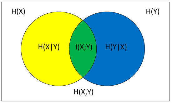
Figure 1.
Venn diagram for various information measures associated with variables X and Y.
Unlike correlation coefficients, mutual information is more general and determines the similarity between the joint distribution of two variables and the products of their marginal distribution. Hence, mutual information of two random variables is invariant to the relationship—i.e., linear or nonlinear—between them.
In [29], Shannon defined the entropy H of a discrete random variable X with possible values xi, i = 1,2,…,n as
in which Pr(xi) means the probability of each value of X. It can be extended to a continuous random variable scenario as
where f(x) is the probability density function of X. To make the concept easier to understand, H(x) can be considered as the average information carried by the random variable X [30].
In [31], mutual information is defined as
From the distribution perspective, it can also be written as
in which represents mutual information of and , is the joint probability of and , and are the marginal probabilities. The continuous version of Equation (9) is presented in the following subsection.
2.3. Estimate Mutual Information through Copula
Equation (9) holds the capability and properties of mutual information. In this equation, both joint distribution density and marginal distribution density exist in this equation. Therefore, it is understandable to consider using copula transformation to simplify the form of Equation (9). This is the inspiration of this work. In this part, a mathematical proof is provided for the feasibility of estimating mutual information adopting copula.
Let us consider be two variables with continuous marginal distribution functions and joint probability density function. Then the mutual information of can be written as
in which, is the joint probability density function and are the marginal distribution functions of . Based on Sklar’s theorem and Equations (3) and (5), the copula of can be represented as
where is the joint cumulative distribution function and are the marginal cumulative distribution functions. Moreover, the density function of copula can be described as
Hence, based on Equation (11), it is obvious that Equation (10) can be rewritten as
Let and consider that are both distributed in the interval [0, 1], then Equation (13) can be simplified as
In this way, instead of estimating , , and without any prior knowledge of the correlation between the variables, the mutual information of random variables can be calculated after finding the probability density function of copula.
2.4. Empirical Copula-Based Mutual Information Estimation (ECMI)
The empirical copula, introduced by Deheuvels in [32], is a non-parametric method where no prior assumption on the relationship of random variables is needed. Besides, considering the feasibility to apply the method for mutual information calculation, an empirical copula is more appropriate compared with other copula family members because of the convenience for understanding and calculating.
According to [33] and Equation (14), the mathematical formula of empirical copula is represented as
where and are the marginal cumulative distribution functions which can be calculated by adopting empirical distribution functions. Taking as an example, it can be expressed as
and the probability density function is written as
In the above functions, N is the size of the original dataset. The function can be approximated by kernel methods [34] which can be generally expressed as
in which, is the input vector, N is the data size, is kernel smoother, is the dimensionality of and is the bandwidth.
In this paper, the mutual information between and can be approximated as Equation (19), which can be described as
in which, represent every subset of their combinations. Since is distributed in [0, 1], the value of when is near zero should be clarified. Considering that, after changing the format, it equals to zero based on L’ Hopital’s Rule as
3. Application: Feature Extraction from Wind Turbine SCADA Data
3.1. Scenario Description
The dataset adopted in this work is a real SCADA dataset covering two months working period of a 2.5 MW wind turbine and the sampling period is 20 s. According to the warning signals, there are 370 alarms during this period. As it is practically impossible to have so many failures or anomalies in such a short period, most of the alarms should be considered only as reminders for operators that there are some ambient turbulences and changes on the wind turbine’s control strategy during operation. In order to figure out the real anomalies in a wind turbine, a performance indicator is created by calculating the deviations between the normal behavior and real observation [35]. This deviation takes the form of Euclidean distance. The behavior of a wind turbine takes the form of power output. To calculate this index, several parameters should be selected from the SCADA dataset to build a regression model in which output power is the target. From the adopted SCADA dataset, output power has the label active power (AP). In the original dataset, there are 53 parameters related to wind turbine subcomponents and the power grid. In this work, 35 parameters which represent wind turbine working conditions are taken into account.
The whole procedure of the application of ECMI is shown in Figure 2. In the calculating process, mutual information between other parameters and active power is estimated in turn and a rank list based on the result is created.
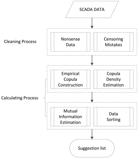
Figure 2.
The procedure of the application of ECMI.
For cleaning process, a typical wind turbine power curve is adopted as a reference. After comparing the observed power curve to the reference, data points which contain negative values for power output are filtered out. Moreover, some bad data points caused by sensor mistakes are also cleaned. The wind turbine power curve from the cleaned dataset is shown in Figure 3.
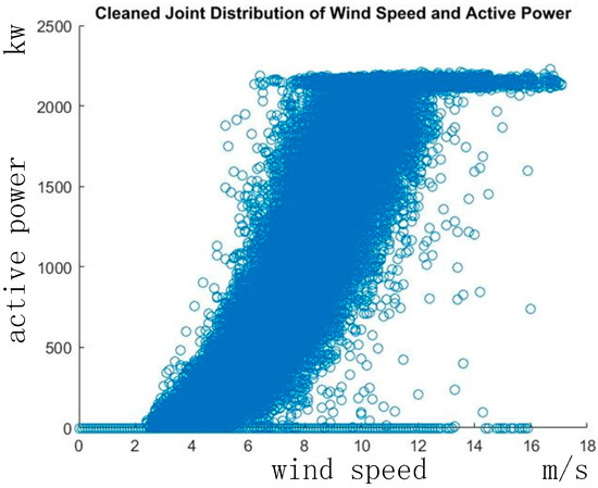
Figure 3.
Power curve from the cleaned dataset.
Besides, as units of each parameter are different, when trying to investigate wind turbine system level behavior, some of the parameters with small value ranges cannot have an equal chance to impact the model. Hence, the data is normalized with Equation (21).
where represents the normalized data vector and means the original dataset.
3.2. Results Based on ECMI
Based on the cleaned dataset, the value of each parameter is divided into 100 bins in [0, 1], empirical copulas of each pair of parameter are constructed and copula density is estimated by adopting kernel smooth method. Figure 4 and Figure 5 show cumulative copula and copula density of variable pairs as (active power (AP), yaw) and (AP, wind speed (WS)).
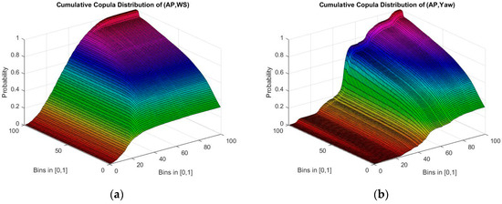
Figure 4.
Cumulative copula distribution of the two parameters. In both figures, X and Y axis represent the bins in [0, 1] and Z axis shows the probability distribution of the copula distribution of the two parameters. In (a), the two parameters are active power and wind speed; while in (b) the two parameters are active power and yaw.
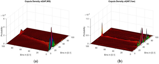
Figure 5.
Copula density of the two parameters. In both figures, X and Y axis represent the bins in [0, 1] and Z axis shows the probability of the copula distribution of the two parameters. In (a) the two parameters are active power and wind speed; while in (b) the two parameters are active power and yaw.
The copula density of (AP, WS) in Figure 5 is the observations of each parameter with the Z axis as the probability value. The distribution of AP and WS proves that the empirical copula process does not change the original information and maintains the physical meaning. Hence, the mutual information estimation can be used as a reference for parameter selection. Moreover, from Figure 5, it can be observed that the probability of copula (AP, Yaw) is much smaller than that of copula (AP, WS). This corresponds to the final result that wind speed ranks higher than yaw in the suggestion list. Since in this work only the components of a wind turbine are taken into consideration, the suggestion list shown in the following table only provides a rank of parameters related to the sub components.
According to [6], parameters which have influence on the output power are selected based on experience. In this paper, nacelle temperature, rotor speed, gearbox oil temperature, hydraulic temperature, generator bearing temperature, wind speed, and pitch angle are suggested for next steps in research. In Table 1, it can be observed that nacelle temperature affects power output, however, it does not rank high enough to be a choice. It means that from mutual information perspective, nacelle temperature does not hold enough information to predict active power. Based on the list, the yaw parameter is recommended for modelling system behavior instead of utilizing nacelle temperature. For wind turbines, this needs further discussion if the misalignment information is available in the SCADA data. According to [36], a wind turbine’s behavior is complex and site dependent. Terrain, wakes, and the coupling among wind turbines may all have impact on a wind turbine’s operation. Besides, considering the gearbox temperature, Gearbox_BearingT1 is recommended due to a higher ranking which implies that it is more closely related to output power. The result shows that ECMI is capable of providing suggestions for parameter selection regarding the difference of each SCADA dataset.

Table 1.
Criticality rank of wind turbine subcomponents based on mutual information.
In the following sub section, the advantages of mutual information based on parameter selection will be discussed by conducting a comparison study between ECMI and other statistical methods for correlation coefficient analysis.
3.3. Comparison Study: The Advantages of Mutual Information Based Parameter Selection
To investigate the statistical relationships among the parameters, some other methods are also available. In this part, Pearson correlation coefficient analysis (PCCA) and kernel canonical correlation analysis (KCCA) are adopted for a comparison study. PCCA is used for estimating the strength of the linear relationship between two variables. KCCA is adopted to assess the strength of the nonlinear relationship between two parameters. The details of these two approaches are described in [20,21].
After applying these two methods to the SCADA dataset, Table 2 shows the results which can be considered as the strength of linear and nonlinear relationship between active power and other parameters. The suggested parameters in [6] are highlighted with red color in Table 1 and Table 2. The differences of the parameters’ locations in the three lists are because that PCCA, KCCA, and ECMI explore different relationships among parameters. For example, in the PCCA-based rank list, the first parameter is Converter_L Current, which has the most linear relationship with output power.

Table 2.
Criticality rank of a wind turbine subcomponents based on PCCA and KCCA.
The advantages of an ECMI-based parameter selection method can be discussed from two perspectives. First, as it is mentioned above, the parameter list based on interconnections among sub-components in a wind turbine is more preferable for field operators. When checking the positions of highlighted parameters in the rank lists, they take relatively higher positions in Table 1. This implies that an ECMI-based rank list and the parameter list based on interconnections among wind turbine’s subcomponents share a similar trend. ECMI method can be used as a supplement when the interconnection based idea is not accurate enough for decision making.
The other advantage of ECMI-based parameter selection lies in the ranks of some parameters. After comparing the results in Table 1 and Table 2, the main differences are the ranks of some parameters such as pitch angle, yaw, ambient temperature, and nacelle temperature.
Both PCCA and KCCA can detect the statistical relation between active power and other parameters. Since pitch angle has significant impact on power output, KCCA-based rank is more reasonable since KCCA is capable of detecting nonlinear relation between variables. When compared to Table 1, ECMI gives an even higher rank than that in KCCA, which shows the effectiveness of the proposed method in detecting nonlinear relationships. Moreover, both PCCA and KCCA failed to provide appropriate ranks of yaw, ambient temperature, and nacelle temperature while all these parameters are often considered important for modeling wind turbines behavior. The reason is that the values of these three parameters are almost stationary, while both PCCA and KCCA are sensitive to parameters which change frequently. In this case, ECMI is more efficient in detecting associations among parameters as it provides a more reasonable rank for yaw, ambient temperature, and nacelle temperature. This should be attributed to the main feature of mutual information that it is a more general method which measures the common information shared by two variables rather than investigating whether they are related linearly or nonlinearly.
From the condition monitoring view, ambient temperature also has an impact on wind turbine power output. Even though this parameter ranks a little bit higher in the ECMI list, it takes a lower position in all three rank lists. However, considering that all the subcomponents are located in the nacelle, the power output is more closely related to nacelle temperature. In three rank lists, nacelle temperature ranks higher than ambient temperature, which is consistent with the field experience.
To evaluate the performance of the ECMI-based parameter selection method, NN is used for testing the capability of the parameters selected from Table 1 and Table 2. The input for the NN is the selected parameters and the target is the AP of the wind turbine. Then the SCADA data regarding all the selected parameters and AP are used to train the NN. After that, the best validation performance is chosen as the indicator which shows the effectiveness of the method. The criteria for parameter selection are:
- Select 10 parameters which rank higher in the three rank lists.
- Whenever there are several parameters regarding to the same sub component, choose the one which ranks higher.
Based on the above criteria, the parameter lists are created and shown in Table 3. In this test, multi perceptron feed forward NN is used to build regression model between AP and the selected parameters through SCADA data. As it is only used for testing, an NN with three layers and 10 neurons in each layer is built. To validate the performance of the training process, Mean Square Error (MSE) is used as the indicator. The training function is scaled conjugate gradient back propagation. After training the NN, the validation performance based on each parameter list is shown in Figure 6. In this case, the method which provides smaller MSE values indicates that it is more accurate in modelling the operation behavior of a wind turbine.
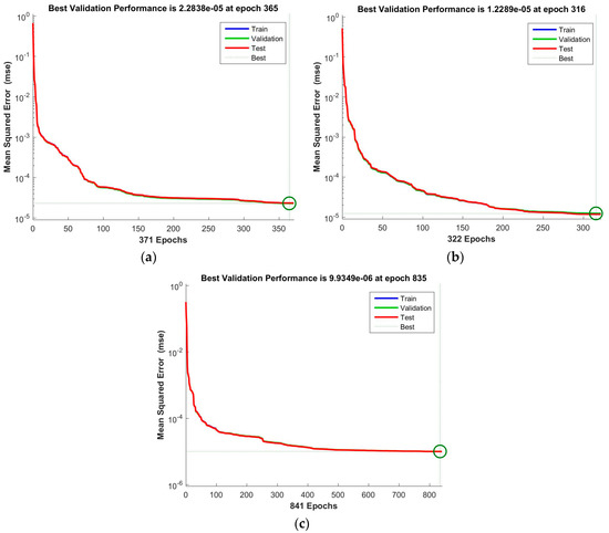
Figure 6.
Best validation performance with three approaches through NN training process. While (a) represent the result based on the PCCA list; (b) shows the result based on the KCCA list; (c) displays the result based on the ECMI list.
From the training results, the MSE based on the ECMI list has the lowest value, , as shown in Figure 6c. The results shown in the KCCA-based test are bigger than the one with ECMI list, however, smaller when compared with the results generated by PCCA list. Hence, the parameter selection method based on ECMI is preferred because it can produce more accurate training results which is very important for wind turbine anomaly detection and condition monitoring.
4. Conclusions
In this paper, an auxiliary decision making method is introduced considering the parameter selection for modeling a wind turbine’s behavior through machine learning techniques. The advantage of utilizing mutual information as an index is presented comparing to other approaches as linear or nonlinear correlation coefficients. After providing background knowledge of both mutual information and copula, a mathematical proof is provided to show that estimated mutual information through copula is more efficient because only copula density needs to be figured out. Then, to make the method more applicable, an empirical copula-based mutual information estimation approach is provided. Besides, real wind turbine SCADA data is adopted for testing the method and the results show the efficiency of the ECMI method.
Afterwards, a suggestion list for parameter selection is provided based on the rank list. A parameter that ranks higher in the list implies that it is more closely related to the target variable. The ECMI method is suitable as an auxiliary method for parameter selection because, while following the physical knowledge of a real wind turbine, ECMI is capable of finding specialties of different dataset which makes the next-step investigation more effective. The advantage of the ECMI-based parameter selection method lies in the fact that no assumptions on statistical relationship among parameters are needed when using it. Moreover, the validation performance after training the NN also shows that the ECMI-based method can produce more accurate results. The future work is to apply this method to different SCADA datasets to test the stability of ECMI.
Author Contributions
Mian Du and Jun Yi conceived and developed the methods; Mian Du and Peyman Mazidi analyzed the data and discussed the results; Lin Cheng and Jianbo Guo contributed theoretical guidance; Mian Du wrote the paper.
Conflicts of Interest
The authors declare no conflict of interest.
References
- European Wind Energy Association. Wind in Power 2015 European Statistics; European Wind Energy Association: Brussels, Belgium, 2016. [Google Scholar]
- Milborrow, D. Operation and maintenance costs compared and revealed. Windstats Newslett. 2006, 19, 1–3. [Google Scholar]
- Yan, Y. Nacelle orientation based health indicator for wind turbines. In Proceedings of the 2015 IEEE Conference on Prognostics and Health Management (PHM), Austin, TX, USA, 22–25 June 2015; pp. 1–7.
- Long, H.; Wang, L.; Zhang, Z.; Song, Z.; Xu, J. Data-Driven Wind Turbine Power Generation Performance Monitoring. IEEE Trans. Ind. Electron. 2015, 62, 6627–6635. [Google Scholar] [CrossRef]
- Sun, P.; Li, J.; Wang, C.; Lei, X. A generalized model for wind turbine anomaly identification based on SCADA data. Appl. Energy 2016, 168, 550–567. [Google Scholar] [CrossRef]
- Lapira, E.; Brisset, D.; Ardakani, H.D.; Siegel, D.; Lee, J. Wind turbine performance assessment using multi-regime modeling approach. Renew. Energy 2012, 45, 86–95. [Google Scholar] [CrossRef]
- Hung, L.P.; Alfred, R.; Hijazi, A.; Hanafi, M. A Review on Feature Selection Methods for Sentiment Analysis. Adv. Sci. Lett. 2015, 21, 2952–2965. [Google Scholar] [CrossRef]
- Guyon, I.; Elisseeff, A. An introduction to feature extraction. In Feature Extraction; Springer: Berlin, Germany, 2006; pp. 1–25. [Google Scholar]
- Nevatia, R.; Babu, K.R. Linear feature extraction and description. Comput. Graph. Image Process. 1980, 13, 257–269. [Google Scholar] [CrossRef]
- Hong, Z.-Q. Algebraic feature extraction of image for recognition. Pattern Recognit. 1991, 24, 211–219. [Google Scholar] [CrossRef]
- Li, H.; Jiang, T.; Zhang, K. Efficient and robust feature extraction by maximum margin criterion. IEEE Trans. Neural Netw. 2006, 17, 157–165. [Google Scholar] [CrossRef] [PubMed]
- Ding, J.; Wen, C.; Li, G.; Chua, C.S. Locality sensitive batch feature extraction for high-dimensional data. Neurocomputing 2016, 171, 664–672. [Google Scholar] [CrossRef]
- Ravishankar, S.; Jain, A.; Mittal, A. Automated feature extraction for early detection of diabetic retinopathy in fundus images. In Proceedings of the 2009 IEEE Conference on Computer Vision and Pattern Recognition, Miami, FL, USA, 20–26 June 2009; pp. 210–217.
- Pamula, V.R.; Verhelst, M.; van Hoof, C.; Yazicioglu, R.F. A novel feature extraction algorithm for on the sensor node processing of compressive sampled photoplethysmography signals. In Proceedings of the 2015 IEEE Sensors, Busan, Korea, 1–4 November 2015.
- Qian, D.; Wang, B.; Qing, Y.; Zhang, T.; Zhang, Y.; Wang, X.; Nakamura, M. Bayesian Nonnegative CP Decomposition-based Feature Extraction Algorithm for Drowsiness Detection. IEEE Trans. Neural Syst. Rehabil. Eng. 2016. [Google Scholar] [CrossRef] [PubMed]
- Medel, J.; Savakis, A.; Ghoraani, B. A novel time-frequency feature extraction algorithm based on dictionary learning. In Proceedings of the 2016 IEEE International Conference on Acoustics, Speech and Signal Processing (ICASSP), Shanghai, China, 20–25 March 2016.
- Gopinath, R.; Kumar, C.S.; Vishnuprasad, K.; Ramachandran, K. Feature mapping techniques for improving the performance of fault diagnosis of synchronous generator. Int. J. Progn. Health Manag. 2015, 6, 12. [Google Scholar]
- Wu, F.; Lee, J. Information Reconstruction Method for Improved Clustering and Diagnosis of Generic Gearbox Signals. Int. J. Progn. Health Manag. 2011, 2, 42. [Google Scholar]
- Steuer, R.; Kurths, J.; Daub, C.O.; Weise, J.; Selbig, J. The mutual information: Detecting and evaluating dependencies between variables. Bioinformatics 2002, 18, S231–S240. [Google Scholar] [CrossRef] [PubMed]
- Benesty, J.; Chen, J.; Huang, Y.; Cohen, I. Pearson correlation coefficient. In Noise Reduction in Speech Processing; Springer: Berlin, Germany, 2009; pp. 1–4. [Google Scholar]
- Hardoon, D.R.; Szedmak, S.; Shawe-Taylor, J. Canonical correlation analysis: An overview with application to learning methods. Neural Comput. 2004, 16, 2639–2664. [Google Scholar] [CrossRef] [PubMed]
- Gábor, J.S.; Rizzo, M.L. Brownian distance covariance. Ann. Appl. Stat. 2009, 3, 1236–1265. [Google Scholar]
- Reshef, D.N.; Reshef, Y.A.; Finucane, H.K.; Grossman, S.R.; McVean, G.; Turnbaugh, P.J.; Lander, E.S.; Mitzenmacher, M.; Sabeti, P.C. Detecting novel associations in large data sets. Science 2011, 334, 1518–1524. [Google Scholar] [CrossRef] [PubMed]
- Kinney, J.B.; Atwal, G.S. Equitability, mutual information, and the maximal information coefficient. Proc. Natl. Acad. Sci. USA 2014, 111, 3354–3359. [Google Scholar] [CrossRef] [PubMed]
- Zeng, X.; Durrani, T. Estimation of mutual information using copula density function. Electron. Lett. 2011, 47, 493–494. [Google Scholar] [CrossRef]
- Póczos, B.; Ghahramani, Z.; Schneider, J.G. Copula-based Kernel Dependency Measures. Available online: https://arxiv.org/abs/1206.4682 (accessed on 12 February 2017).
- Sklar, A. Fonctions de Répartition à n Dimensions et Leurs Marges; Université Paris: Paris, Fracne, 1959; Volume 8, pp. 229–231. [Google Scholar]
- Nelson, R.B. An Introduction to Copulas; Springer: Portland, ME, USA, 2006; pp. 7–42. [Google Scholar]
- Shannon, C.E. A mathematical theory of communication. Bell Syst. Tech. J. 1948, 27, 623–656. [Google Scholar] [CrossRef]
- Carter, T. An Introduction to Information Theory and Entropy; Complex Systems Summer School: Santa Fe, NM, USA, 2007. [Google Scholar]
- Gray, R.M. Entropy and Information. In Entropy and Information Theory; Springer: New York, NY, USA, 2013; pp. 36–37. [Google Scholar]
- Hominal, P.; Deheuvels, P. Estimation non paramétrique de la densité compte-tenu d’informations sur le support. Rev. Stat. Appl. 1979, 27, 47–68. [Google Scholar]
- Charpentier, A.; Fermanian, J.-D.; Scaillet, O. The estimation of copulas: Theory and practice. In Copulas: From Theory to Applications in Finance; Risk Books: London, UK, 2007; pp. 35–62. [Google Scholar]
- Nagler, T.; Czado, C. Evading the curse of dimensionality in multivariate kernel density estimation with simplified vines. J. Multivar. Anal. 2016, 151, 69–89. [Google Scholar] [CrossRef]
- De Vieira, R.; Sanz-Bobi, M. Failure Risk Indicators for a Maintenance Model Based on Observable Life of Industrial Components with an Application to Wind Turbines. IEEE Trans. Reliab. 2013, 62, 569–582. [Google Scholar] [CrossRef]
- Castellani, F.; Astolfi, D.; Sdringola, P.; Proietti, S.; Terzi, L. Analyzing wind turbine directional behavior: SCADA data mining techniques for efficiency and power assessment. Appl. Energy 2017, 185, 1076–1086. [Google Scholar] [CrossRef]
© 2017 by the authors. Licensee MDPI, Basel, Switzerland. This article is an open access article distributed under the terms and conditions of the Creative Commons Attribution (CC BY) license ( http://creativecommons.org/licenses/by/4.0/).