Pressure Losses in Hydraulic Manifolds

Abstract

Hydraulic manifolds are used to realize compact circuit layout, but may introduce a high pressure drop in the system. Their design is in fact oriented more toward achieving minimum size and weight than to reducing pressure losses. This work studies the pressure losses in hydraulic manifolds using different methods: Computational Fluid Dynamic (CFD) analysis; semi-empirical formulation derived from the scientific literature, when available; and experimental characterization. The purpose is to obtain the pressure losses when the channels’ connections within the manifold are not ascribable to the few classic cases studied in the literature, in particular for 90° bends (elbows) with expansion/contraction and offset intersection of channels. Moreover, since CFD analysis is used to predict pressure losses, general considerations of the manifold design may be outlined and this will help the design process in the optimization of flow passages. The main results obtained show how CFD analysis overestimates the experimental results; nevertheless, the numerical analysis represents the correct trends of the pressure losses.

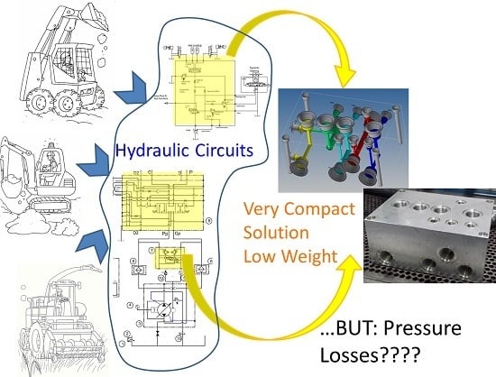
1. Introduction

Hydraulic system layouts, in particular for mobile applications such as off-road machines, have to both fit in the narrow spaces available in vehicles and guarantee functionality with acceptable efficiency. Efficiency of hydraulic systems is a key topic, discussed by researchers and the industry in a common effort to reduce dissipations which are quite extensive in this kind of system. In [1], Murrenhoff et al. describe the most recent energy-efficient hydraulic architectures for mobile applications, spanning from the “valve-systems”, in which independent metering or digital valves can be used instead of the traditional ones, as well as “pump-controlled” systems, which eliminate the directional valves, and energy recovery systems, which use energy from braking or lowering of loads to recover hydraulic energy with accumulators and hydraulic motors. Other authors focused on the applications of one energy-saving architecture on a specific off-road vehicle, such as analyzing the independent metering system impact on the energy saving during some typical duty cycles, applied to excavators or forwarder machines, as in [2], or even to agricultural tractors, as in [3]. All this interest is well legitimized when considering that the average efficiency of hydraulic systems in industrial applications is 50% and drops to 21% for mobile applications, according to [4]. The main losses come from the hydraulic pumps and motors and from the valves controlling the actuators but, since even a little improvement in energy reduction may have a great impact on fuel consumption reduction, every aspect of the hydraulic system deserves attention and may positively contribute to efficiency. Efficiency may be increased significantly by reducing the pressure losses caused by the fluid flowing in pipes and manifolds. The consequence of high pressure drop is in fact the increasing of the pressure level in the system far beyond the one needed to perform the requested work. Moreover, pressure drop causes the additional generation of heat in the system that must be removed opportunely, thus requiring additional input energy.

Hydraulic manifolds house compact circuit layouts made of internal channels and screwed valves. They can be of two types: the monoblock design, holding all the passages and valves for an entire system; and the modular-block one whereby each modular block supports only one or two valves and contains interconnecting passages for flow going to the actuations. Generally, it is connected to a series of similar modular blocks to build up a complete system. Hydraulic manifolds are used both in industrial and mobile applications; however, the problem of the lack of room is more critical in the mobile applications and, as a consequence, it is in this case that we expect more complicated internal passages and higher pressure losses. The design of this kind of element can be extremely important to reduce the pressure level needed in the circuit, though in the past the attention was mainly focused on the need to design the minimum block size and to guarantee adequate mechanical strength of the component.

As stated in [5], the design to obtain the minimum size often implies a rather complicated set of drillings to bring about fluid circulation between external ports of the components. Another priority in the past was given to the ability to design the block in an automated way, also considering the difficulties and the limits of manufacturing [6].

This took place in an era when the fuel costs, fuel availability and the pollutant emissions, due to the engine driving the hydraulic power unit, were not considered a priority. Nowadays, the designing process of this kind of component must include the pressure loss evaluation and reduction, thus necessitating analysis of flow through the internal passages.

It must also be considered that the general problem of pressure loss evaluation for several channel geometries, involving bends, intersections and complex paths, is of interest for the design of the casing of the positive displacement machines used in fluid power mobile applications. Often these casings house two machines (for example, the main and boost pumps; the pump and motor of an hydrostatic transmission); the passages for the fluid, however, may be very complex. Results coming from the analysis performed in this work may, hence, be useful also in this case.

Empirical or semi-empirical formulas reported in past literature cannot be applied to the different combinations of geometries that can be found in the manifolds. Hence, the pressure loss evaluation in the internal connections of a manifold is not a foregone task; the internal channels may present multiple bends with different curvature values and different diameter sizes. While many studies have been done in the past on single and double 90°-bend (elbow) passages, finding loss coefficients for the evaluation of pressure drop can be difficult due to generalized rules for the design. For a singular particular case, experimental measurement or Computational Fluid Dynamic (CFD) analysis are the only resources to have a correct estimation. Moreover, 2D and 3D CFD analyses have proven to be affordable when applied to study the flow through pipes, as shown, for example, in [7]. Some examples of the application of CFD analysis on manifold, even if for a different type of application than the one here analyzed, can be found in [8,9,10,11]. They are all examples of how CFD analysis has been helpful to analyze the flow inside solar collectors, typically characterized by rather complex geometries, and they demonstrate how CFD analysis is able to identify critical regions that can compromise the efficiency in heat transfer as in [8]; or to study the design parameters that can more strongly affect the flow distribution and consequently also the heat transfer, as in [9,10]. Finally, in [11], a consistent review of different methods to study the flow in manifolds is presented, where CFD, discrete models and analytical models are analyzed. In this last paper, the author also states that often a CFD model suitable for optimizing the geometry of a manifold can be too expensive from the point of view of time and computational effort. This is true also in the case analyzed in this work because, in industry, the designers typically do not have time and suitable tools to perform well enough. It is for this reason that the authors here decided to use a commercial CFD code for the numerical analysis, which is easy to manage and popular in the industry. It was therefore possible to analyze the benefits and the limits of the tool used and, at the same time, to define general considerations on the basis of the qualitative results obtained, which have been confirmed by the experimental analysis.

While experimental measurement is more expensive and needs at least one prototype, CFD analysis uses a virtual prototype; nevertheless, the computational time requested in order to have very accurate results may be high. The combination of the two analyses in order to find some rules to apply to the design of the manifold, seems to be a good way to help industry designers, who typically need to meet harsh market requests.

This work studies the pressure losses in hydraulic manifolds using different methods: CFD analysis, empirical and semi-empirical formulation from the literature, when available, and experimental measurement. This first analysis on a basic 90° bend, or elbow, has allowed for calibration of the CFD analysis via comparison with published data; then, the analysis is extended to the elbows with expansion/contraction/offset geometries. In particular, as far as the authors know, there are no available results or discussions about this kind of geometry, which is, however, often found in manifolds as a result of the design process. The results obtained allow the drawing of some guidelines for the design of the manifold channels, in particular for 90° elbows, and a critical discussion of the results of the CFD analysis that, if extensively used during the design, allows for a drastic reduction in the number of experimental tests, thus optimizing the flow through the channels. In the next step of the research, the attention will be focused on more complex connections composed of multiple 90° elbows and crossing channels with crossing angles different from 90°.

The paper is subdivided into the following paragraphs: the first section reviews the past literature results; the second one presents the CFD analysis description applied to some test cases also studied in the literature to validate the accuracy of the analysis; the third section presents the experimental setup; the following section discusses the results obtained for a series of geometries not examined in the literature; and the final section reports the results obtained from the CFD analysis of pressure losses when considering two elbows; after a discussion about the numerical-experimental data comparison, the conclusions draw some considerations regarding manifold design.

2. Discussion of Past Literature

Flow in pipes is a topic extensively studied in the past, especially in the years 1930–1960; bends of different geometries were experimentally and theoretically analyzed because of their considerable importance in the design and analysis of fluid machinery and piping systems. However, as stated also in [12], where an extended review of past literature is provided, we can find wide variations in loss coefficients quoted by the various investigators. Moreover, because actual details of their test conditions are often missing, it is not possible to correct their results to provide meaningful data.

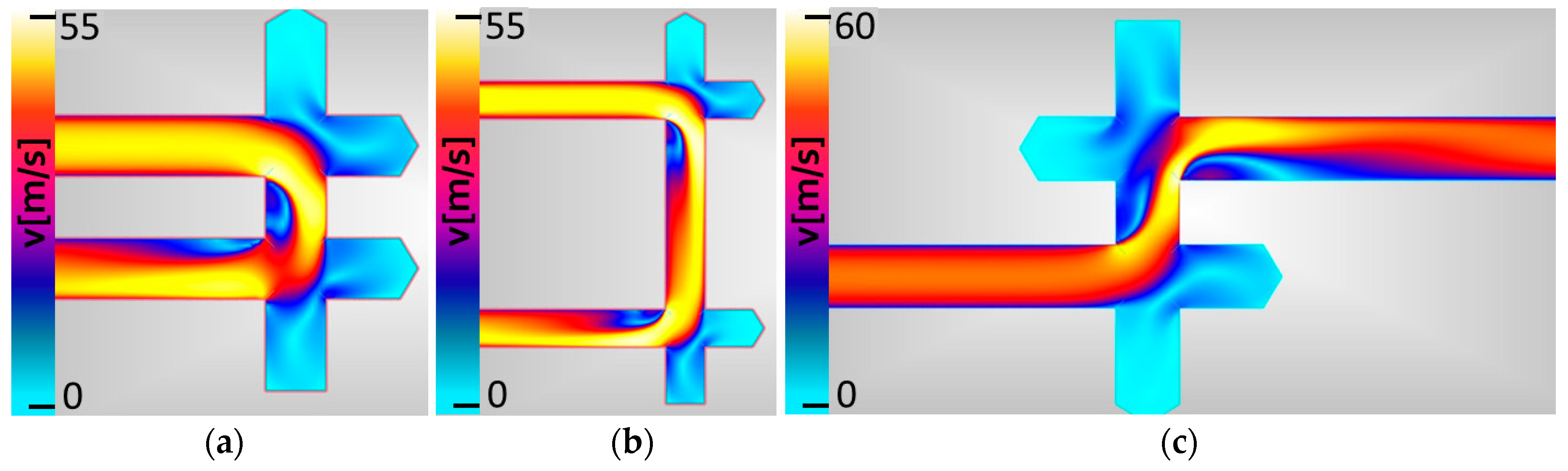
For the single elbow, many results can be found; for example, in [13,14] the change of direction of flow in curved channels causing the formation of centrifugal forces, directed from the center of curvature toward the outer wall, is shown. Therefore, upstream of the elbow, the passage of fluid from the straight part to that curve is accompanied by an increase of outer wall pressure (decrease of the speed) and a decrease in the internal wall (increase of the speed). The “diffuser” effect leads to flow separation from both walls: from the inner wall, it is intensified by the inertia forces which act in the curved zone and tend to move the particles towards the outer wall. The vortex zone that is formed with the separation from the inner wall propagates axially and radially, reducing the main flow area. The pressure drop is mainly caused by the presence of vortices and is calculated through the sum of the local loss coefficient plus the friction coefficient. An observation in [13] states that when the output section is greater than the input one (expansion), the diffuser effect is intensified leading to an increase in vortices and flow separation, i.e., a decrease in velocity and an increase in the pressure downstream of the elbow. 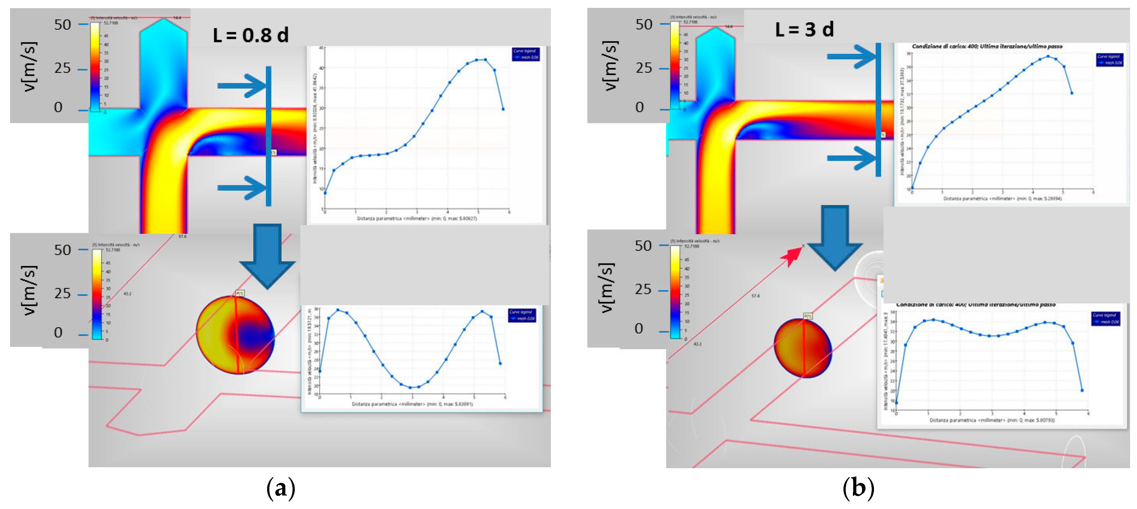In Figure 1, the qualitative velocity maps (yellow = highest speed value) and profiles near the curvature (A) and at a distance L = 3∙d (d is the channel diameter) from the curvature (B) are shown: they were determined by the authors of this paper with the CFD analysis of one 90° elbow to rebuild the considerations found in [14].

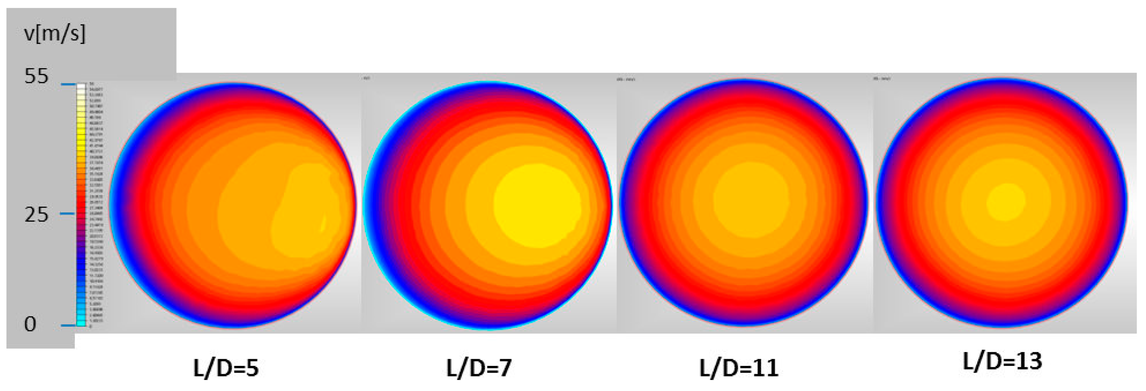
Murakami et al., between the end of the 1960s and the end of the 1970s, published several works on the flow through bends. The single elbow is in particular analyzed in detail in [14]’s assessment of the flow speed through a channel of diameter d with an elbow. Defining a distance L which is zero in correspondence to the elbow and which increases following the flow direction, it was stated that the maximum axial speed of flow is located near the section L/d = 0.1, shortly after the elbow. Then the speed is gradually restored to normal distribution near the downstream section L/d = 10. Again, the authors noted that the formation of an irregular secondary flow downstream, involves sections between 0.8 < L/d < 3, while the normal secondary flow distribution is restored for L/d ≥ 3. It was thus observed that, after a certain length downstream of the elbow, the symmetric axial velocity profile is re-established. If a second elbow is positioned at that distance L/d = 13 or more from the first one, there is no interaction between the two losses (see also Figure 2).

Moreover, in [14] the authors analyzed the case of two elbows at a varying distance L_m and with different orientation of the second elbow compared to the first one, thereby changing the relative angle between the axis of the first and last part of the pipe (twisting angle). The geometry varies from a U shape (twisting angle 0°) to an S shape (twisting angle 180°). The authors found that, if the distance between the elbows is lower than five times the diameter, the upstream elbow can strongly influence the downstream one and the loss coefficient is no longer constant with the twisting angle, reaching a maximum for values spanning in the range of 120°–140°. They found that the distance at which the presence of the elbows stops influencing the fluid flow is lower for the U and S shapes compared to the others. The U shape is the one that introduces the lowest pressure drop. In [15], the authors confirm these results applying CFD analysis to an hydraulic manifold with the bend geometries described in [14]. These results were also confirmed in [16,17], where, moreover, CFD analysis was used to analyze the pressure drop through a complicated internal passage with multiple elbows, for which the empirical formulation cannot be applied. Comparing the numerical results with the experimental ones, CFD was assessed as a good method to evaluate pressure drop according to the authors, even if a certain gap between the numerical and experimental results is evident.

3. Computational Fluid Dynamic (CFD) Preliminary Analysis

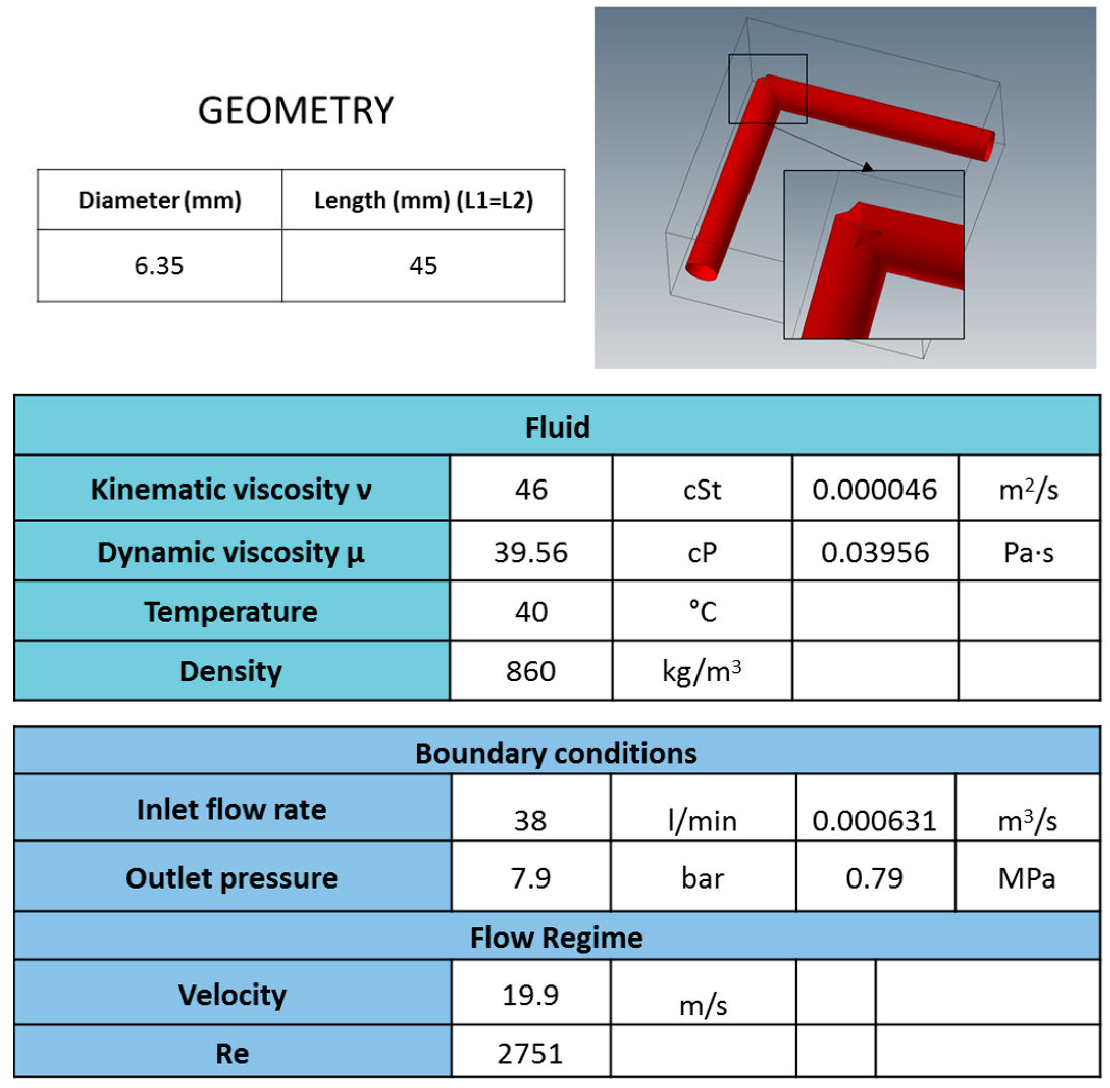
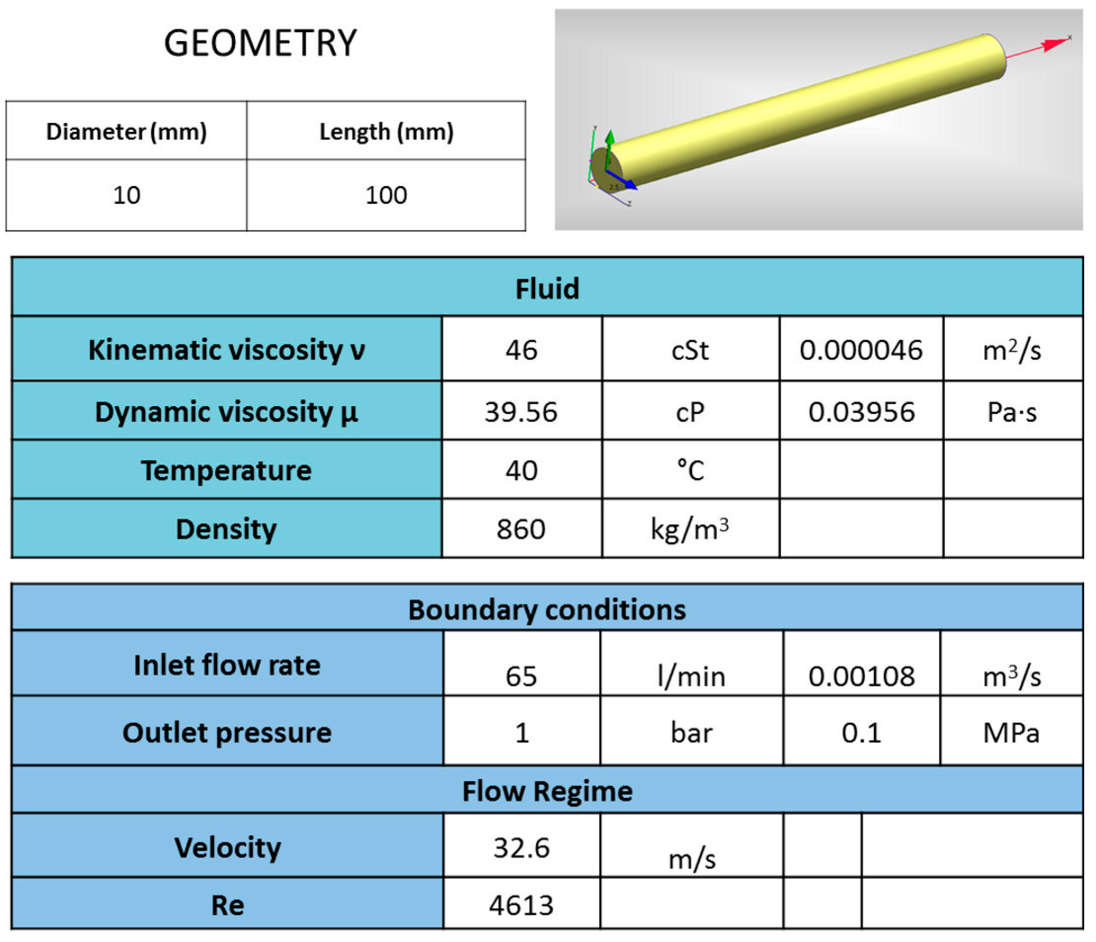
In this section, two basic test cases are used to compare the results of analytical and semi-empirical formulations with the results coming from the CFD analysis; the aim is to guide the CFD mesh generation and the choice of adopted turbulence model. The first test case considered for calibrating and validating the CFD analysis was the straight channel, as reported in Figure 3, in which also the fluid properties and test conditions are specified.

The analysis was performed using commercial software that integrates the volume meshing and fluid dynamic analysis of a component [18]. The results were compared with the one derived from the use of the Poiseuille law, since the Reynolds number in this case is quite low (

Table 1. Poiseuille law and the value of the parameters for the test analyzed.

Poiseuille Law	μ (Pa·s)	d (m)	Q (m3/s)	L (m)	Δp (MPa)
	0.03956	0.01	0.0005	0.1	0.0081

).

The fluid in the simulations is an ISO VG 46 mineral oil (kinematic viscosity 46 cSt at 40 °C) with a density of 860 kg/m³; it is the same fluid available in the test rig described in the following and used for the experimental analysis. The imposed boundary conditions were atmospheric pressure at the outlet of the system and a flow rate at the inlet. An additional portion of the channel (entry region) was also considered in the analysis in a way that, after this region, the velocity profile became fully developed and continued unchanged. An estimate of the entry length for different types of flow depends on the Reynolds number Re and the channel diameter d and is given by ~0.06∙Re∙d for laminar flow while it is approximated with different formulas for turbulent flow, in which the influence of Re number is weaker; in many pipes’ flow of practical engineering interest, the entrance effect are insignificant after a pipe length equal to 10∙d [19].

An extruded mesh was chosen as the most suitable to be used for this geometry. This type of grid is made of triangular elements stretched into multiple layers of prismatic elements through the length of 3D parts with a uniform cross-section. The choice of this structured mesh has two advantages: reduction of elements generated and a lower computational cost for the simulations; more precision of the results in geometries with a uniform cross-section, i.e., aligning cells with the flow allows reduction of the diffusion of the calculated quantities among the cells. A sensitivity analysis of the influence of the extruded mesh on the results has been performed taking note of the number of elements along all fluid−wall interfaces that can be critical for accurate flow prediction.

Using an opportune extruded mesh to discretize the geometry, introducing an appropriate entry length (90∙d, where d is the pipe diameter) to guarantee a fully developed velocity profile, and considering laminar flow, the analysis of the pressure drop across the pipe has given a result analogous to the theoretical formulations: 0.0087 MPa. This test case was used to analyze the impact of the two main factors that affect the solution in terms of pressure drop calculated with the CFD analysis: the mesh properties and the entrance length at the inlet needed to obtain a fully developed velocity profile at the inlet.

Since the extruded mesh appears to not be the best choice for any geometry considered in this paper, this test case was also used to refine the automatic mesh generator that adopts an unstructured mesh in order to obtain the same result as above. A study of an alternative suitable mesh was necessary: the unstructured mesh gave the closest results with respect to the extruded mesh when the ratio between the element size and the minimum channel diameter size, in the test case considered, was less than 0.06. Moreover, under this value, the result remains unchanged. This is the rule followed in creating the mesh in the succeeding test cases.

The second test case analyzed was a simple elbow for which again empirical and theoretical formulations already allow evaluation of the pressure drop. The details of geometry, fluid properties and boundary conditions are reported below. The mesh near the internal walls (boundary layer mesh) is structured, characterized by four layers with a layer factor of 1.2 (multiplying it by the local isotropic length scale for the surface, the layer height is determined) and, setting an automatic function, it is possible to manage the growth rate of the layers. With these settings, a sensitivity analysis for the mesh size was performed: in particular, the ratio (mesh ratio) between the element size and the minimum channel diameter in the geometry considered was decreased from 0.2 to 0.06, a value under which the pressure drop remains substantially unchanged (modifications are lower than the measurement accuracy, 0.0335 (MPa)) and the computational cost increases considerably. Information about the number of elements are reported in

Table 2. Pressure drop in the elbow test case, calculated with different turbulence models.

Mesh Ratio	0.2	0.1	0.08	0.06	0.05
N° of elements	41 K	256 K	508 K	1460 K	1746 K
N° of nodes	16 K	84 K	145 K	384 K	484 K
Δp from CFD analysis with k-ε (MPa)	0.895	0.89	0.87	0.81	0.8
Δp from CFD analysis with k-omega (Mpa)	0.8	0.805	0.775	0.8	0.775
Δp from CFD analysis with low-Re k-ε (MPa)	0.845	0.775	0.905	1.2	1.5

.

To obtain a fully developed velocity profile at the inlet, an opportune function available in the software has been used: this option simulates a fully developed velocity profile and avoids the addition of an inlet channel that would slow the calculation.

The connection between the channel ends is done in a way that there is no extension of one channel beyond the other one. Compared to other types of intersection, in particular with extension of the inlet channel beyond the outlet or with extension of both channels, this geometry is characterized by the lower pressure drop values, according to the CFD analysis. Figure 4 shows the geometry, fluid properties and test specifications used.

In addition to the CFD simulations, the results from a semi-empirical formulation were calculated: the total pressure drop is split in a distributed loss along the two straight sections, calculated with the Blausius formulation, and in the sum of the distributed and concentrated loss in the elbow, according to the approach described in [13]. The relative error between the CFD results and the formula in this test case was about the 3% and it was considered as a good agreement when applied to the analysis of manifold pressure drop.

This test case was also used to analyze the performance of the chosen turbulence model, the standard k-ε model. This is a general-purpose model that performs well across a large number of applications; although it is not the most accurate; see, for example, the analysis performed in [20] on a diffuser—it is robust and, in most cases, the solution easily converges, and for these reasons is still widely used. Other available turbulence models were tested: low Re k-ε model is generally used for a pipe in which flow condition is between laminar and turbulent, but the analyses run with this model requested more iterations to reach a fully converged solution. In general, this model may not be as stable as the k-ε one. SST (Shear Stress Transport) k-ω model (recommended for external aerodynamics, separated or detached flows, and flow with adverse pressure gradients) is robust across a wide range of flow conditions, though it does not use wall functions, meaning that it simulates turbulence all the way to the wall. To use this method effectively, the mesh needs to be very fine in the boundary layer region. These methods were all tested in the commercial code used and the results were compared: despite a finer mesh needed to obtain convergence and a computational time consistently increasing, the final pressure drop values calculated differ from the k-ε model pressure drop of about 3% in the k-ω case, while the low Re k-ε model case has a convergence problem and determines pressure drops that are increasingly significantly. For that reason, it was chosen to continue the analysis using the k-ε turbulence model (and this is also the choice made by the industry in most of cases).

Moreover, no cavitation modelling is available in the adopted commercial software.

4. Experimental Setup

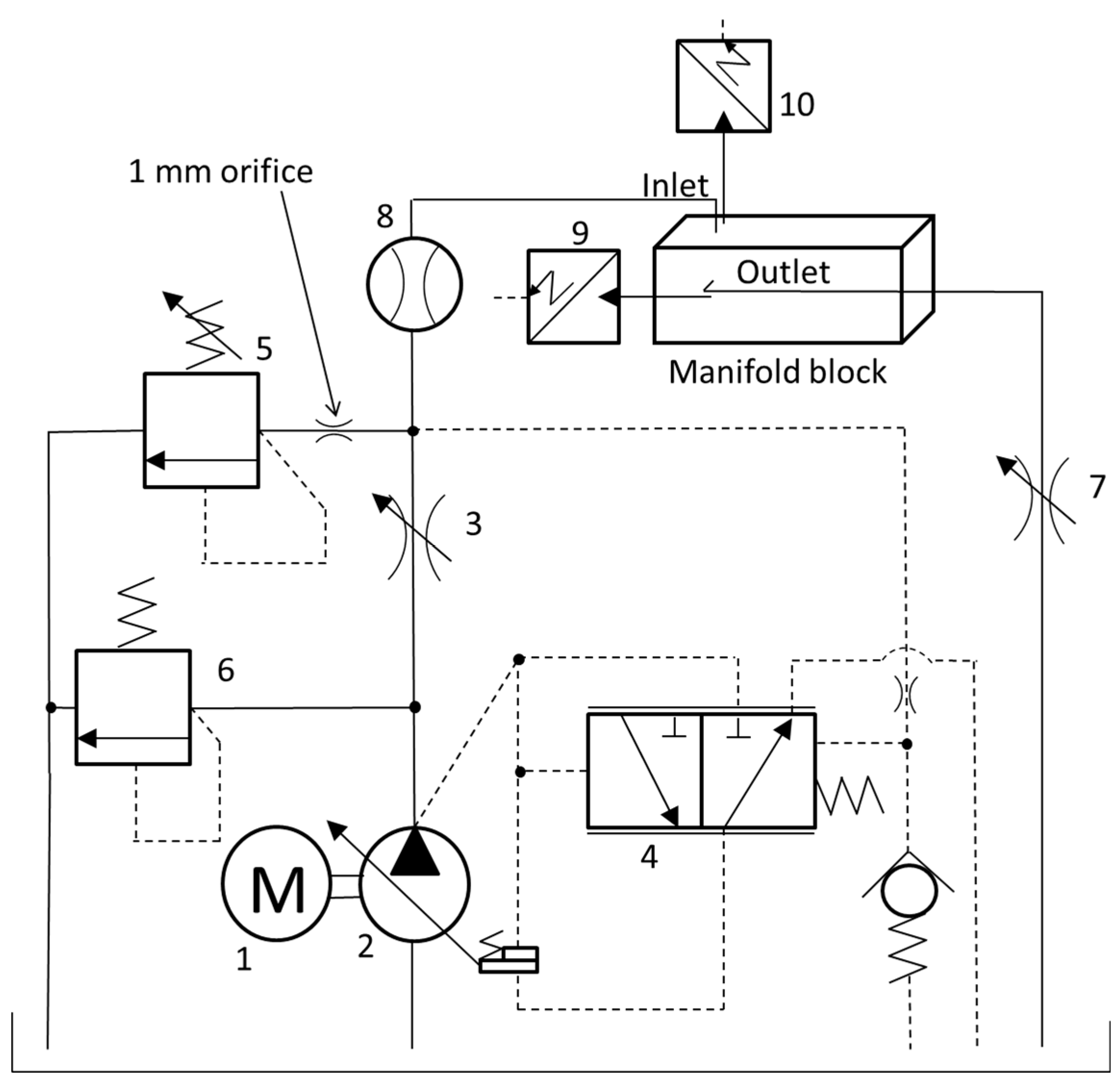
To compare and verify simulations results, the selected geometries have been reproduced in two manifold blocks designed opportunely to have Reynolds number values above the laminar region of flow. This was evaluated considering the range of flow rate available in the test rig (maximum 65 L/min). The manifold blocks were experimentally characterized at the University of Modena and Reggio Emilia in the Fluid Power Laboratory. The lab provides the power unit of the test bed represented in Figure 5. The power supply is a hydraulic power unit constituted by:

• 15 kW electric motor, 4-pole, operating at 380 V, 50 Hz ((1) in Figure 5);
• A variable displacement swashplate axial piston pump with flow and pressure compensator (maximum flow 65 L/min, maximum pressure 28 MPa) ((2) in Figure 5);
• An external gear pump feeding the off-line circuit dedicated to the cooling and filtering of the fluid (not represented in figure); the heat exchanger allows maintaining a controlled temperature (38 °C ± 2–3 °C).

The fluid power generator group is a typical load-sensing group in which a variable flow regulator (3) is placed in the pump delivery line and the pressure drop across this orifice acts on the flow compensator (4) of the pump against a preloaded spring, thus generating a variation in pump displacement. Manually regulating the flow regulator (3) leads to the increase of the flow rate, which can be further raised acting on the regulation of the relief valve (5), thus increasing the pressure downstream of the orifice (3) and inducing a reaction of the pump with increase of flow. Hence, with this configuration, it is possible to set the flow and measure the pressure drop across a passage. Valve 5 is not used as a relief valve but, rather, to calibrate the pressure in the delivery line; it is an extra function that was designed in the test rig to illustrate how a load-sensing system can work.

The relief valve (6) has the highest pressure setting in the test rig and operates only for safety in case of pressure peaks in the delivery line. The variable orifice (7) can be adjusted eventually when cavitation occurs during the passage through the manifold in order to provide sufficient backpressure.

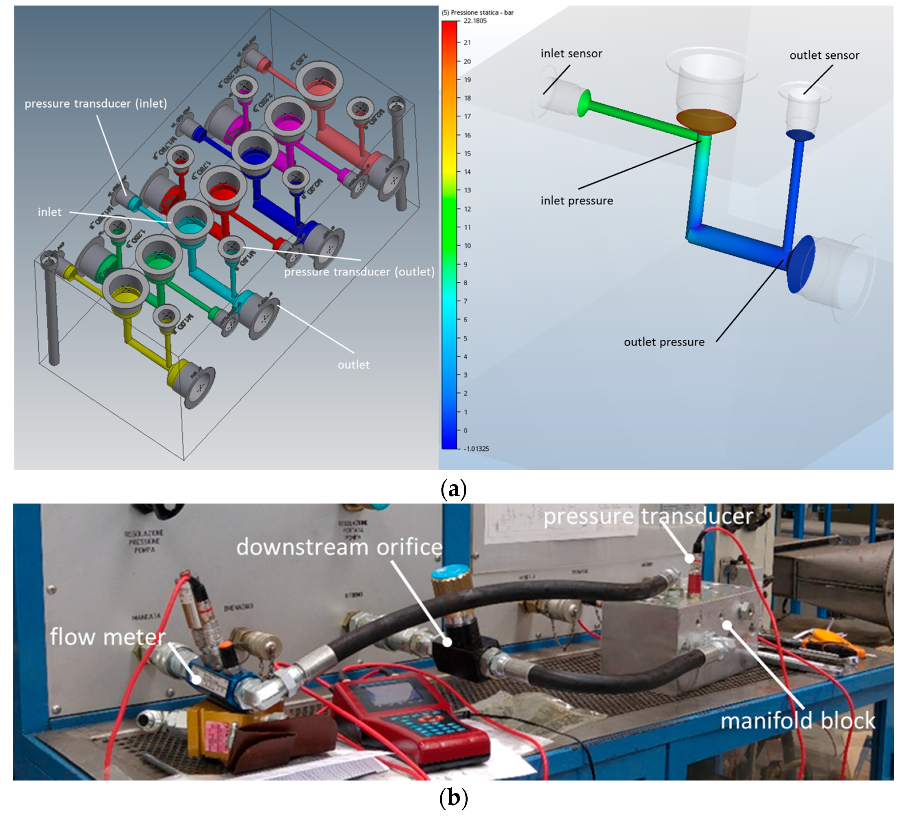
The manifold block, designed with a dedicated commercial software [21] and shown in the upper part of Figure 6 (CAD model and position of the sensors, (a)), has several fittings to connect the delivery of the pump/return to the tank to the inlet and outlet of each internal passage. There are also pressure taps onto which transducers are directly screwed and holes, realized in the four corners, to secure with screws the manifold to the test bed. Several fittings and two short hoses are used to connect the manifold to the test bed delivery and tank lines ((b) in Figure 6).

In the text rig there are two portions of hose which end with a connector for the hydraulic manifold. The connectors (90° bend with threaded ends) are positioned at a distance from the internal elbow higher than 13∙d, where d is the internal diameter. Significantly, as found in the literature, when two elbows are positioned at this distance they no longer influence each other. The entry length before the internal elbow is ten times bigger than the internal diameter, and this distance is enough to have a fully developed velocity profile when the flow is considered turbulent [18].

The instrumentation used for measurements and data acquisition includes two pressure sensors ((9) and (10) in Figure 5), a flow meter ((8) in Figure 5) and a portable measuring system to convert and read measurements [22]. Their characteristics are reported in

Table 3. Sensors’ main characteristics.

Sensor/Data Acquisition	Range	Accuracy
Piezoresistive pressure sensor	0–6 MPa, relative	0.5% FS (0.03 MPa)
Piezoresistive pressure sensor	−0.1–0.6 MPa, relative	0.5% FS (0.0035 MPa)
Turbine flow meter	7.5–75 L/min	2.5% FS (1.69 L/min)
MULTI SYSTEM 5060 PLUS	8 channels	-

.

The pressure transducers are mounted on the manifold, upstream and downstream of each elbow analyzed, while the flow meter is positioned upstream of the manifold (Figure 5 and Figure 6).

The values are taken with the digital multi-channel measuring system and then downloaded to the computer for analysis.

The global uncertainty on the pressure drop measurement, that is an indirect measure in this case because two independent pressure sensors are used, was calculated summing the accuracy of the two pressure sensors used and dividing this for the pressure drop measured (as, for instance, in [23]). From this, the percentage uncertainty can be easily determined. Considering the accuracy of the pressure sensors, the uncertainty in the experimental measurement of pressure drop under 0.1 MPa is unacceptable (total accuracy of 0.0335 MPa), while progressively decreasing when the pressure drop increases. For instance, at 0.1 MPa of pressure drop the uncertainty becomes 33.5%; at 0.5 MPa of pressure drop the uncertainty becomes 7%; at 1 MPa it is about 3%. The experimental results are reported without error bars for the sake of clarity and better reading of the diagrams.

5. Single-Elbow Geometries

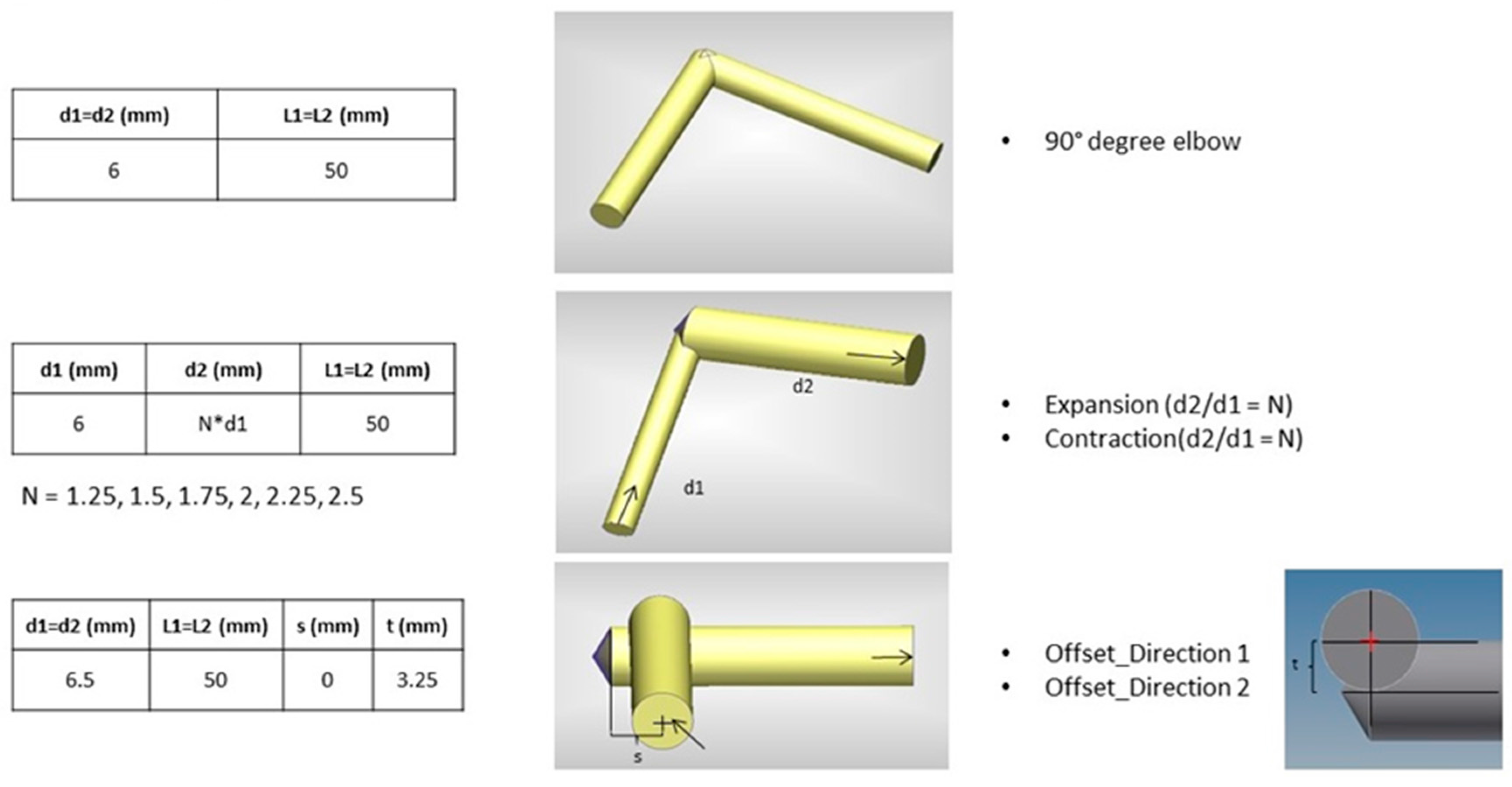
The tests reported in this section concern geometries with one elbow (90° bend). Figure 7 shows the chosen geometries which are a simple elbow, an elbow with expanding and contracting flow passages and finally an elbow with an offset between the axis of the two channels. As stated in the introduction of this work, the geometry chosen (single elbows with expansion/contraction/offset and, in the next section, double elbows) is often obtained in a manifold block as a result of the design process, but the designer is rarely aware of the difference in pressure losses that characterizes each of them. The manifold, in fact, realizes a real circuit layout and the flow passages can be rather complicated but, substantially, they consist of one, two or more elbows at different distances. The diameters of the elbows have been chosen in a way to obtain the Reynolds number spanning from about 300 to 5000 with the range of flow 5–65 L/min available for experimental tests; turbulent flow in the manifold are establishing already for rather low Reynolds number values.

In the CFD analysis the mesh was generated as described in Section 3 and the analysis was carried on varying the flow rate range from 5 to 65 L/min. The fluid properties at 40 °C adopted are reported in

Table 4. Fluid properties.

Kinematic viscosity ν	46	cSt
Dynamic viscosity μ	39.56	cP
Temperature T	40	°C
Density ρ	860	kg/m3

.

For general understanding and comparison between the here-obtained results and others in the literature, the data in the following are shown using dimensionless variables. The pressure drop is non-dimensioned with respect to $\frac{1}{2}\cdot \rho \cdot v^2$, where ρ is the fluid density and v is the flow velocity defined as the maximum flow rate in the tests performed over the reference flow area at the inlet of the geometry considered. The flow rate is non-dimensioned with respect to the maximum value used in the tests. In that way, the results are comparable with the ones that we can find in literature (for example, in [13,14]).

5.1. Simple 90° Elbow

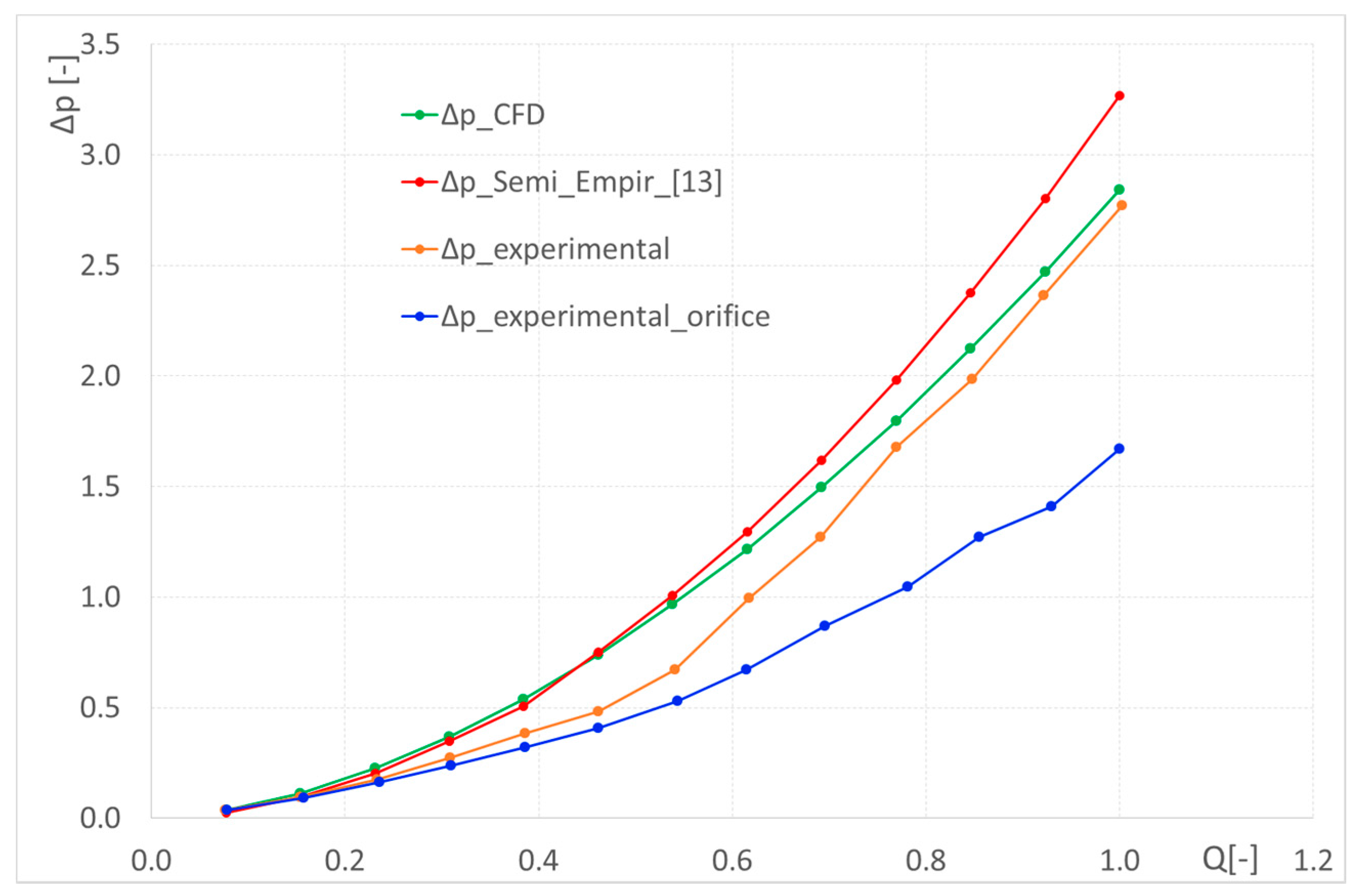
This geometry represents one of the typical channel intersections within a manifold, in particular between channels with the same diameter, disposed at 90° angle and with crossing axes.

Figure 8 compares the results, in terms of pressure drop, from the experimental test (fluid temperature is maintained between 37 °C and 39 °C), CFD simulations and the results calculated (Δp_Semi_Empir_ [13]) with the semi-empirical Blausius formula combined with the Idelchik approach ([13]). Two experimental curves are reported because they were measured in one case regulating the orifice (7) in Figure 5 to create backpressure (Δp_experimental_orifice) while in the other case the orifice was left fully open (Δp_experimental). The experimental error reduces to negligible values for the higher flow rate values, but when the error is very high at low flow rates, the pressure drop is small enough not to be significant to the manifold designers.

Both CFD analysis and the semi-empirical approach proposed in [13] overestimate experimental losses; however, the gap with CFD results appears smaller. In the first experiment (orange line in Figure 8), for flow rate values equal and higher than 35 L/min, there is an evident change in the curve shape of the pressure drop; this variation as well as the low value of pressure measured at the outlet may be signals of cavitation occurrence. For this reason, the measuring was repeated reducing the section area of the orifice (7) in Figure 5 at the outlet pipe section downstream of the manifold, until the outlet pressure is regulated well above the atmospheric value. The added restriction in fact provides the necessary backpressure and may help to avoid cavitation (blue curve in Figure 8).

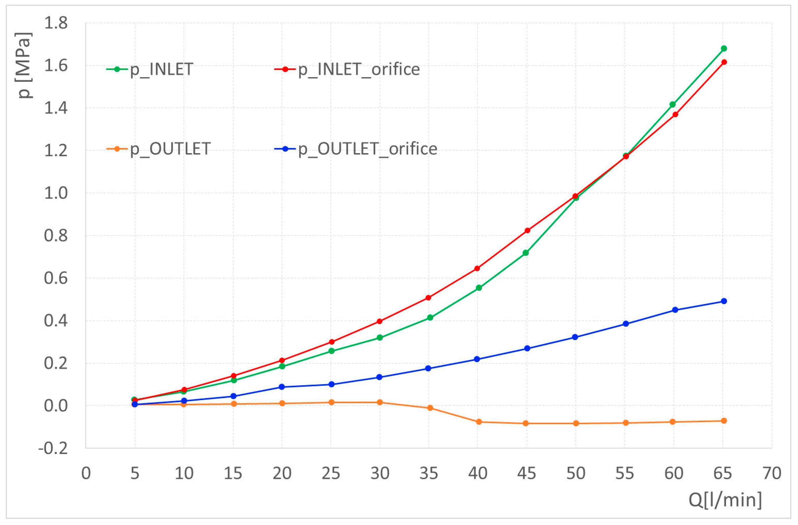
Let’s compare the inlet and outlet pressure trends in the two cases in Figure 9, where the measured trends of pressure are reported (here pressure is not non-dimensioned to improve understanding). While the outlet pressure significantly changes in two experiments, the inlet one follows more or less the same trend and values. It is evident that, in the experiment without the downstream restriction of the flow passage, the cavitation occurrence and the consequent gas bubble formation contribute to decreasing drastically the flow area, causing an increase in pressure drop (also shown in [17]).

This happened every time we found aeration/cavitation during the fluid passage, and these considerations are valid also for the elbows with expansion/contraction shown in the following section.

The pressure losses calculated with CFD analysis, instead, are not sensitive to the backpressure value.

5.2. Expanding and Contracting Elbow

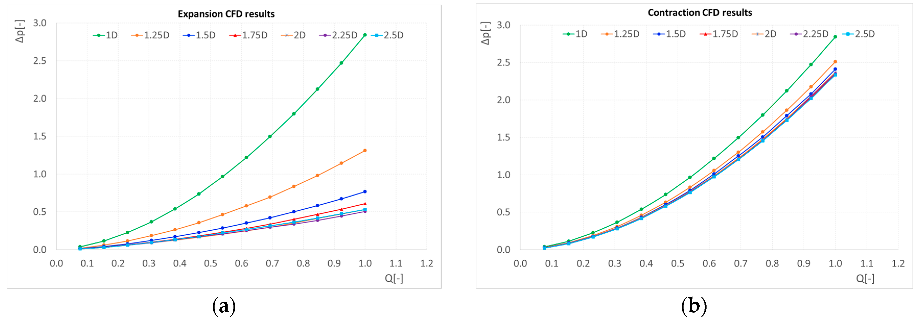
This type of geometry represents the intersections between channels with different diameters: the analysis has been done with the fluid flowing from a smaller to a larger section (expansion) and in the opposite direction (contraction). We have analyzed intersections with an expansion/contraction ratio (the ratio between the greater and the smaller diameter) varying from 1.25 to 2.5. In this case, the comparison is made between CFD simulations and experimental tests, since results from similar geometries in scientific literature were not accessible.

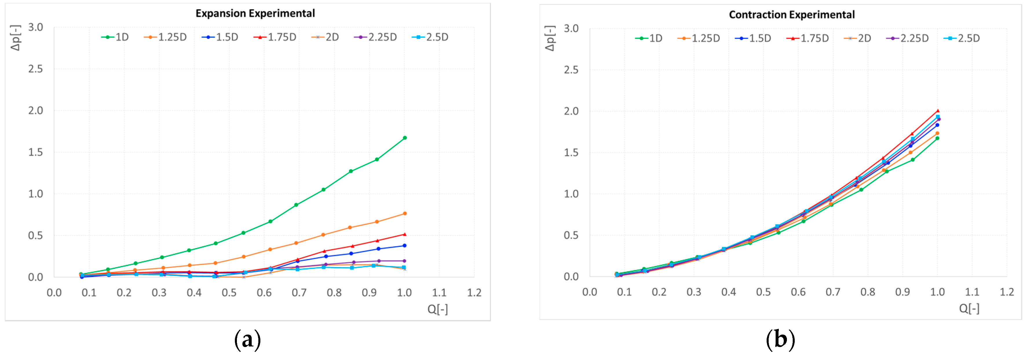
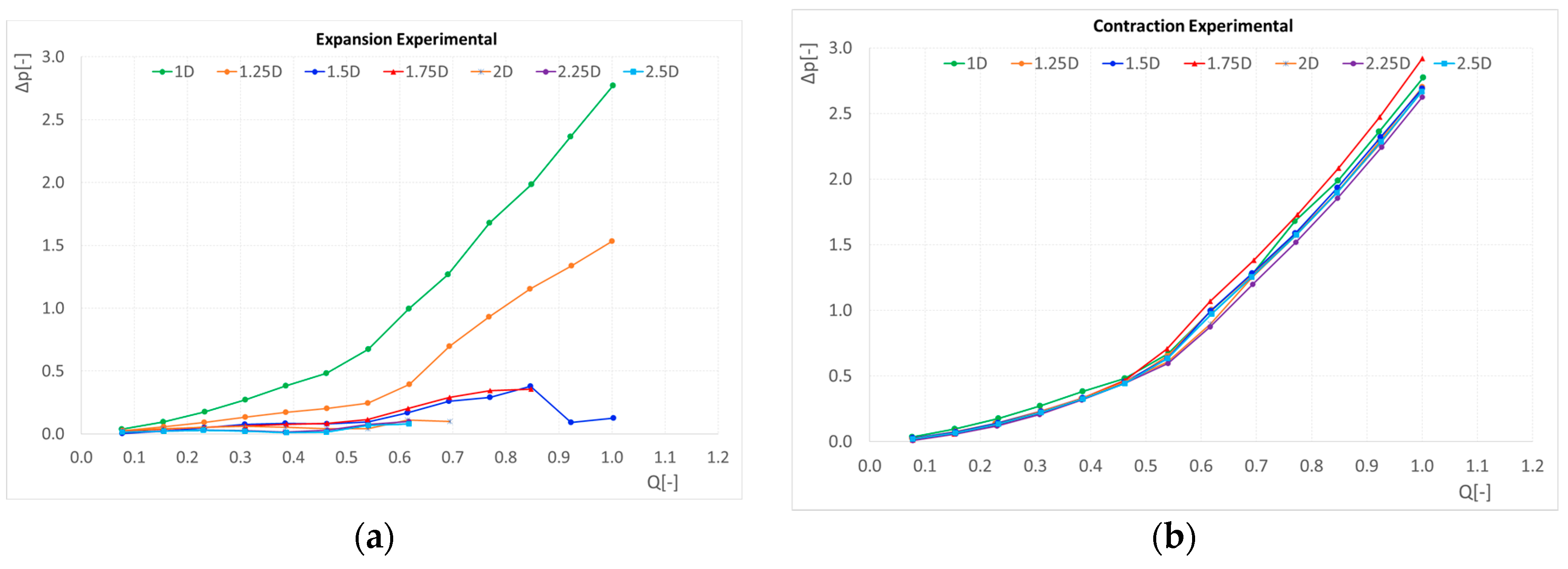
Figure 10 shows the pressure drop curves calculated by the CFD analysis, Figure 11 reports the pressure drop measured adjusting the orifice at the outlet section, and finally Figure 12 is relative to the pressure drop measured without restricting the outlet orifice. In this last case, some pressure losses resulting as “negative” have not been plotted in the diagram. The reason for these negative values is that the range of the pressure sensor at the inlet is limited at the atmospheric value (0–6 MPa, relative); we thus have a sensor that is not able to measure under 0 MPa relative at inlet and an outlet sensor that can measure until −0.1 MPa relative. When the pressure loss in the elbow is very low (strong expansion with cavitation), and the inlet pressure is also dropping under the atmospheric value, the pressure drops measured can be “negative” only as a consequence of the pressure range of the sensors.

The gap between CFD results and experimental results is reduced when looking at the experiment in which the downstream orifice was not restricted, since in the experiment in which cavitation is occurring the pressure drops are higher than in the other case, and generally CFD results overestimate the measured pressure drop.

In the experiment without the restriction of the downstream orifice, the cavitation effect on pressure drop is visible when the flow rate is equal or higher than 35 L/min when the fluid temperature is about 38–40 °C, while this “critical value” of flow is higher when the test is repeated at 30–32 °C; this is expected since the vapour pressure of a fluid increases with the fluid temperature and hence cavitation may occur for lower flow rate values.

Generally speaking, a great reduction of pressure drop characterizes the expansion elbow, also found in the CFD analysis, although with no marginal gap with respect to the experimental results obtained avoiding cavitation. In the case of contraction elbow, the pressure drop trends are not very sensitive to the change in contraction ratio (this is true both for CFD and experimental results) and CFD results follow the experimental trends always overestimating them.

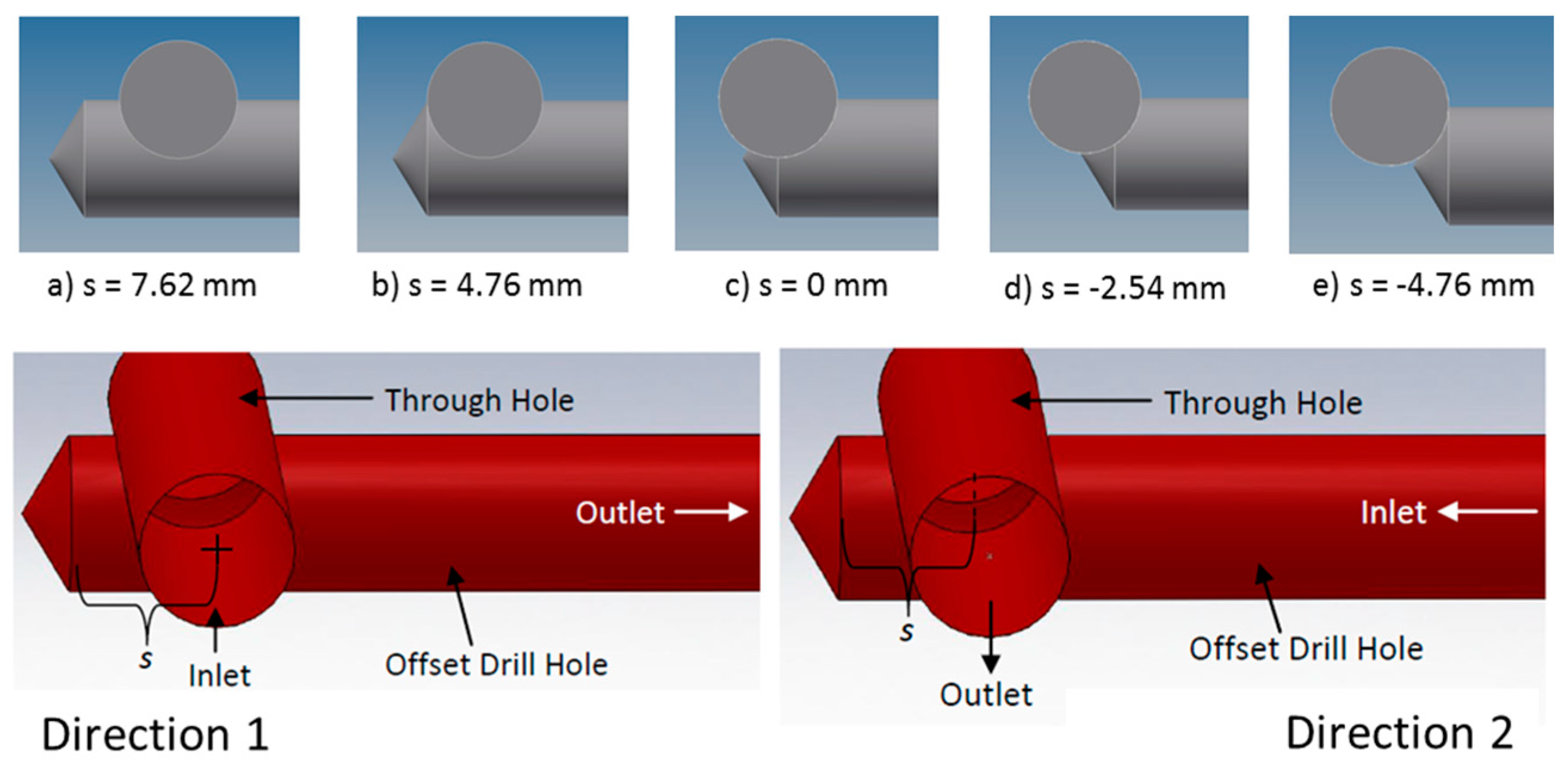
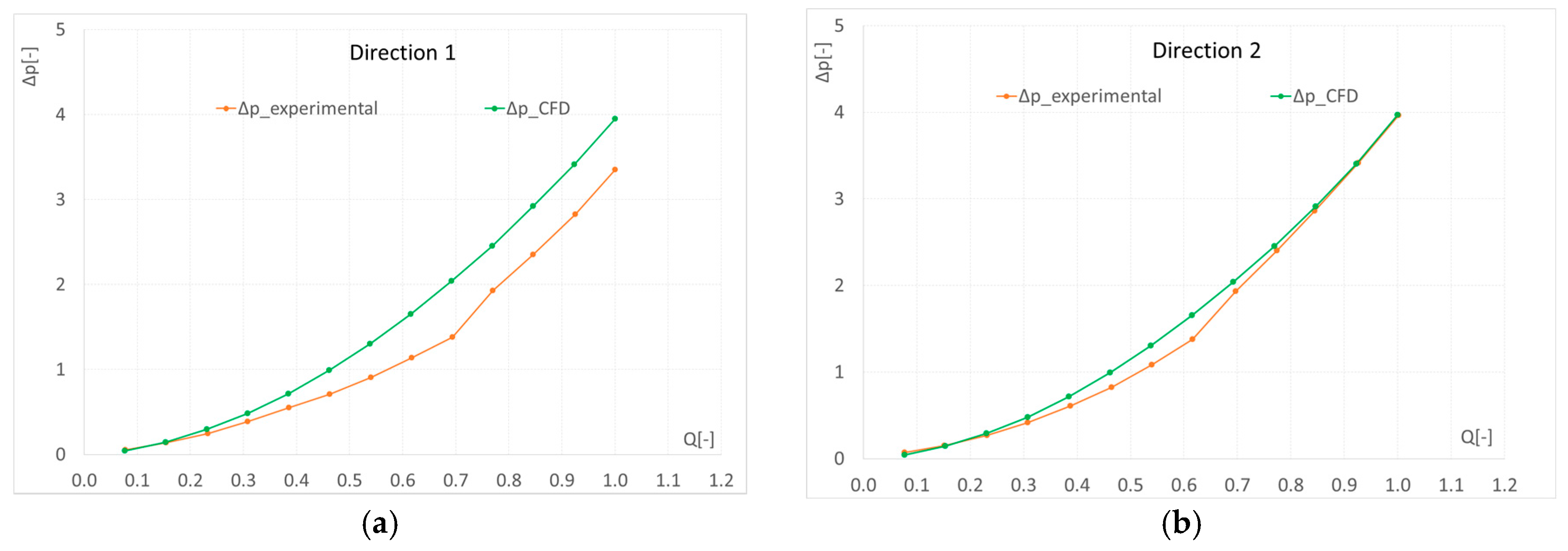
5.3. Offset Elbow

This geometry represents intersections between channels with no crossing axes, having the same diameter; the analyzed geometry is reported in Figure 7 wherein the parameters t and s, which define the offset connection, are shown. Experimental tests were done in both flow directions, which are shown in Figure 13 together with the variation of the length s in the geometries analyzed.

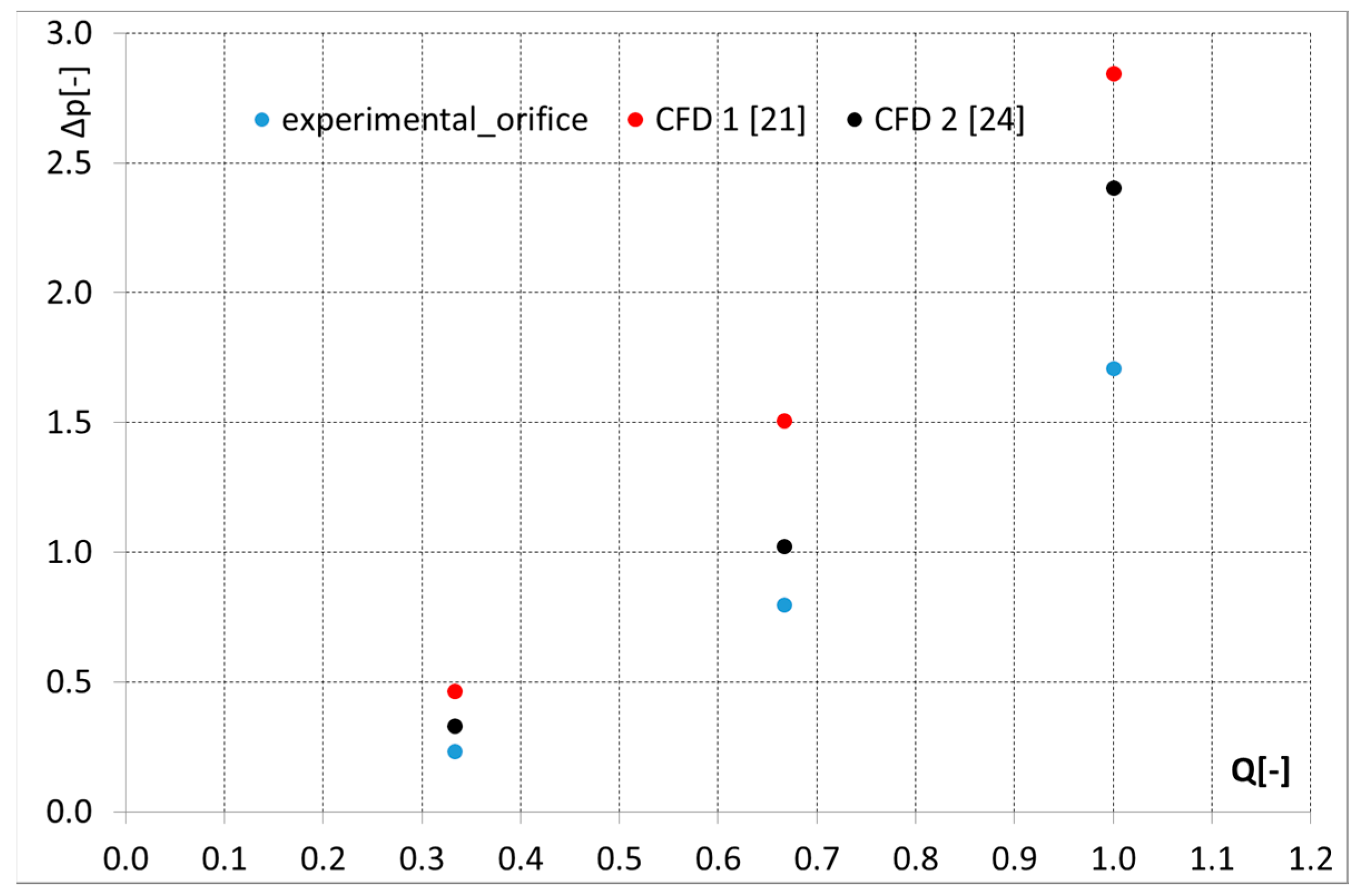
Figure 14 shows that in the case t equal to the channel radius and s = 0, the pressure drop trends are quite the same than the ones in channels with crossing axes. CFD results are slightly higher than the experimental ones obtained without the restriction of the downstream orifice. In addition, CFD simulation does not suggest differences in values between one direction and the other (the curves are overlaid), since the geometry is symmetrical and simulations are ideal. Instead, experimental results differ a little from each other, mainly because cavitation in one case occurs for lower values of flow rate.

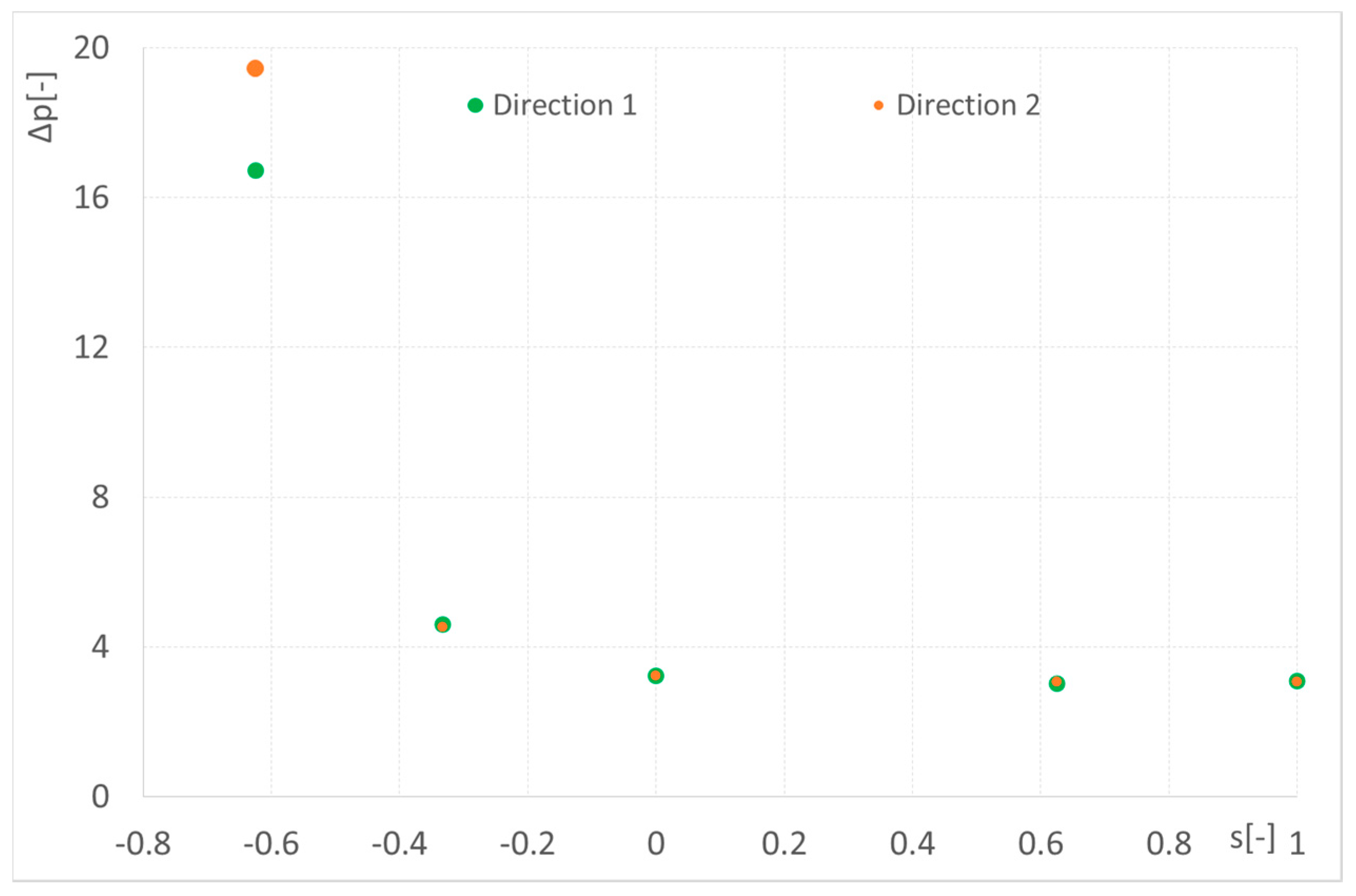
Figure 15 shows the pressure drop variation with the distance s (in this test the flow rate was 75 L/min and the diameter of the pipe of 9.525 mm). As can be expected, the values increase as the intersection area between the channels reduces (negative s), while it is reduced to a constant value when this area stops changing (positive s).

5.4. General Considerations

Results from CFD simulations show that the virtual analysis is able to depict the correct trend of pressure drop-flow rate curves in all the different geometries following, at a “certain distance”, the experimental results. The difference between experimental and CFD results normally rises with the increase of flow rate and pressure drop. The deviation is, however, quite high and always with an overestimation of CFD simulations compared with the experimental measurements; this overestimation can also be found in [16,17]. In the experimental tests, as expected, the flow becomes turbulent at lower velocities (and hence Re values) than those identified for a straight tube; in fact, the elbow modifies the velocity distribution in the channel and causes a pressure drop. The semi-empirical formulation for elbows, when available, can be inaccurate in the estimation of the pressure drop as well as the CFD results that we have obtained in the analysis, as illustrated in Figure 8. Nevertheless, we can highlight that the use of CFD analysis, after having defined the correct mesh, may easily allow a manifold designer to qualitatively find the trend of pressure drop—flow rate curves for different geometries and to reasonably choose the best one for energy saving.

Specifically, looking at the geometries analyzed, some considerations can be made:

• Elbow with expansion: in the first experimental tests, cavitation and aeration strongly affect the pressure drop-flow rate curves. After repeating the tests restricting with the downstream orifice, the trends maintain a parabolic shape only for the lower expansion ratio, 1.25; whereas for higher expansion ratio values, the pressure drop trends are very low (and the accuracy of the measurements are very small in these cases). Instead, CFD results for the elbow with expansion show that the pressure drop-flow rate trend is always parabolic.
• With an expansion ratio of 1.25, the pressure drop is drastically reduced with respect to the normal elbow and both experimental and CFD results show this trend;
• In the case of a contraction elbow, there is no significant variation of the pressure drop with the contraction ratio (this is true both for CFD and experimental results) and CFD results still follow the experimental trends in always overestimating them;
• Looking at the offset elbow, attention must be paid to the fact that, with relatively high distances s and t, the intersection area between the channels may be drastically reduced, thereby causing very high pressure drop values.

6. Two Elbows

As described in Section 2, the results for the geometries of two elbows are reported here to assess the ability of CFD simulations to depict the correct pressure drop trend, when evaluating the flow through the manifold block in the case of more complex connections. The double-elbow geometries analyzed differ from each other by twisting one extremity of the pipe from a 0° twisting angle (U shape) to 180° (S shape). In Figure 16 some images obtained from the CFD analysis show qualitatively the flow patterns which resemble the ones reported in the literature (for example, in [13,14]).

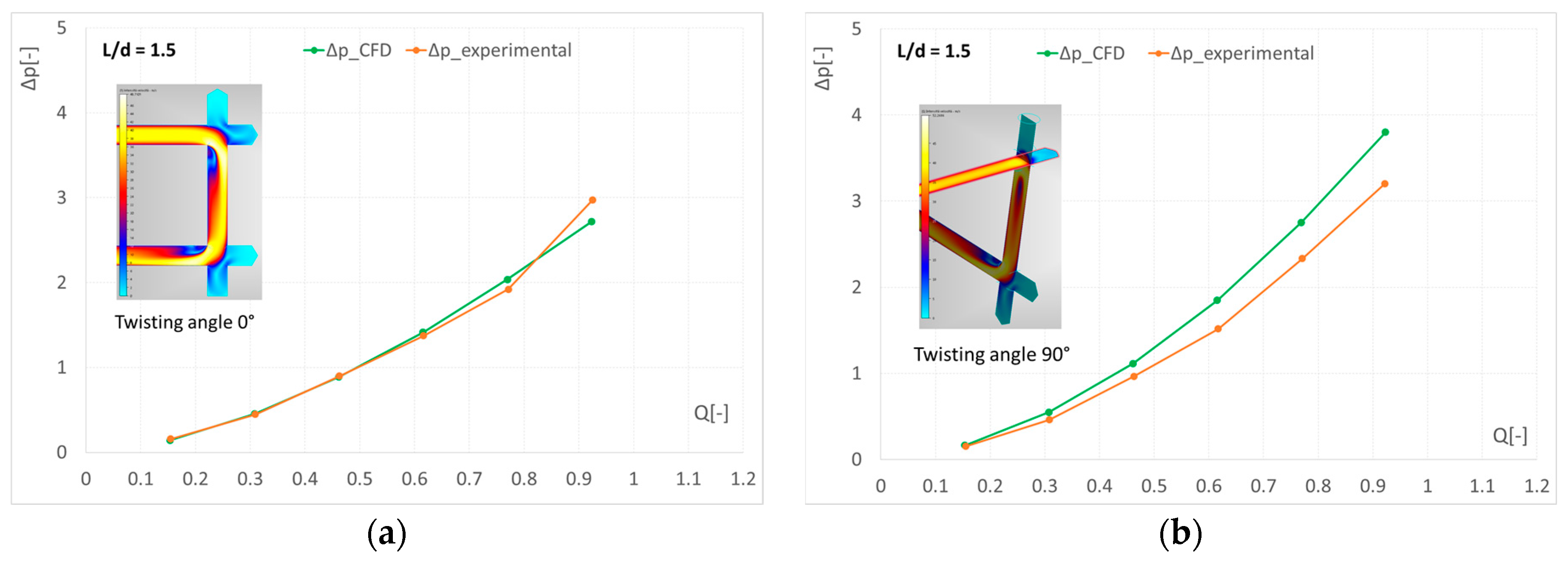
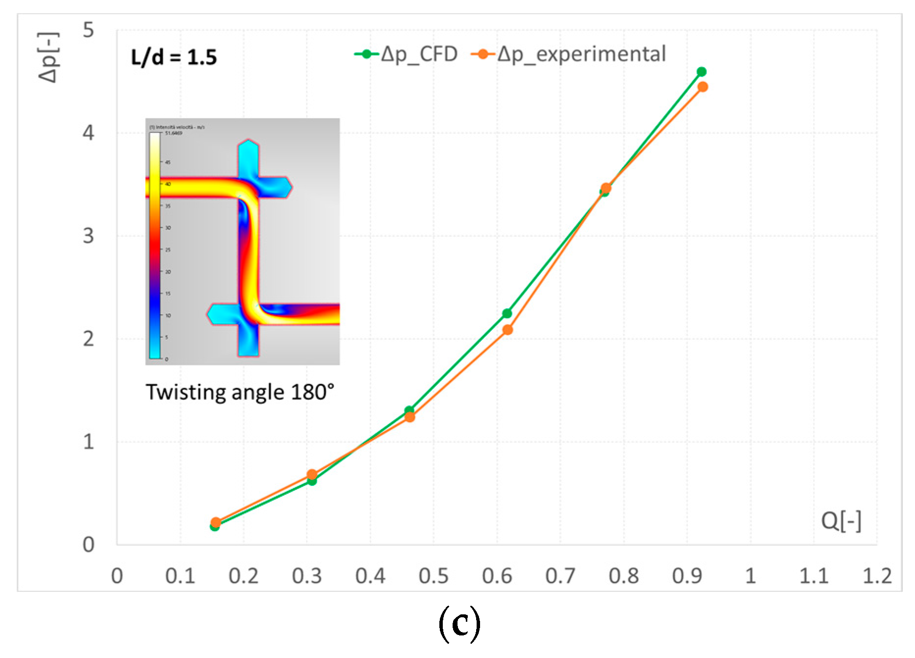
The U shape is characterized by the fact that a high velocity of flow (yellow) is induced after the first elbow at the outer wall of the straight section and a vortex at the inner wall creates a favourable way for the flow to access the second 90° elbow. With the S shape, the second elbow forces the flow to turn against the turbulence determined by the first elbow.

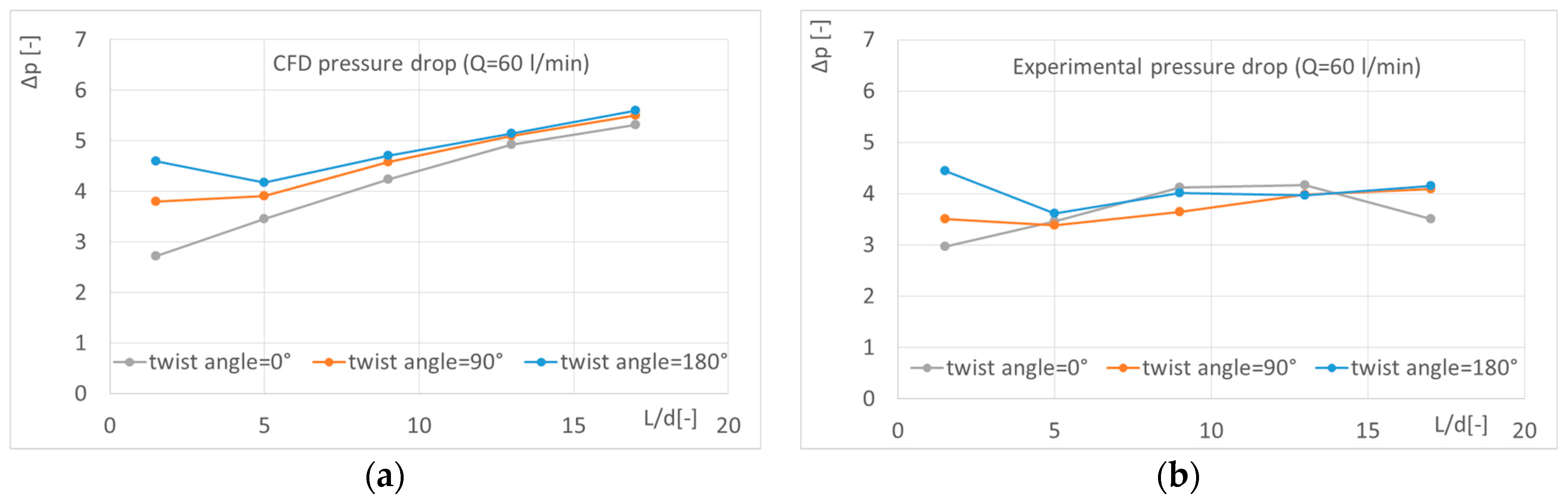
In the following, the three distinct cases are considered: two elbows with a twisting angle equal to zero, two elbows with a twisting angle equal to 90°, and two elbows with a twisting angle equal to 180°. The distance L between the elbows is kept constant at the value L = 1.5·d, d being the channel diameter. The pressure drop curves, both determined with CFD analysis and experimentally measured, are shown in Figure 17 in a dimensionless shape. It is confirmed, as it is reported in literature, that the U shape determines the lowest pressure drop when the two elbows are very close to each other. The experimental values and CFD values are very similar in the case of two elbows in a series, certainly more in agreement than the “one-elbow case”.

As noted in [13,17], the pressure drop, as a function of the dimensionless distance L/d between the two elbows and considering a constant flow rate (60 L/min), has different trends according to the twisting angle between the two elbows (Figure 18).

The CFD results present an increasing trend of pressure drop with the distance L/d, which is slightly different from the trend of the experimental results. Nevertheless, at a distance L/d = 13, the pressure drop values in the three cases analyzed are the same thus demonstrating that from this distance on, the two elbows are independent from one another. As a consequence, when L/d is growing and the two elbows become independent, the deviation between experimental and numerical data increases at values similar to the ones found when analyzing only one elbow. Finally, taking into account the combination of two elbows, the CFD analysis is able to qualitatively predict the correct behaviour of flow, as discussed in the past literature.

In terms of the experimental analysis, the backpressure here is naturally caused by the second elbow and only few cases present cavitation during the experimental test. Only in these few cases were the measurements repeated with back pressure. It was also tested that, without cavitation occurrence, the difference in pressure drops measured with or without the backpressure is of the order of 10⁻² (MPa) (same order of the measurement accuracy), i.e., the pressure drop is not sensitive to the backpressure if cavitation is not occurring.

The comparison between experimental and numerical results is better here than the single-elbow case, at least when the two elbows are near enough (L/d < 13), whereas the error is still high as the two elbows are at a distance L/d > 13, i.e., when the double elbows behave as two elbows not influencing one another. We have credited this to the turbulent k-ε model that seems more robust in the two-elbow test.

7. Discrepancy between Numerical and Experimental Results

In this section, we consider the numerical results obtained with [18] (no cavitation modelling) and the experimental results obtained in the case “single elbow” with no cavitation and “double elbows” (not affected by cavitation in the test realized, since backpressure is always present in the cases analyzed). We would like to compare here the results obtained with another widely used commercial software program [24]—quite well known in literature for being robust—with the aim of better exploring the discrepancy between the numerical results, obtained with [18], and the experimental ones. The first test case chosen was the single elbow with expansion/contraction ratio equal to 1. CFD analysis 1 was performed as described previously, with k-ε turbulent model; CFD analysis 2 was performed with software [24], with the same mesh characteristics used in CFD analysis 1 and both k-ε and low Re-k-ε turbulent models. It was chosen to plot in Figure 19 only the results obtained with low Re-k-ε turbulent model because the residuals in that case were lower.

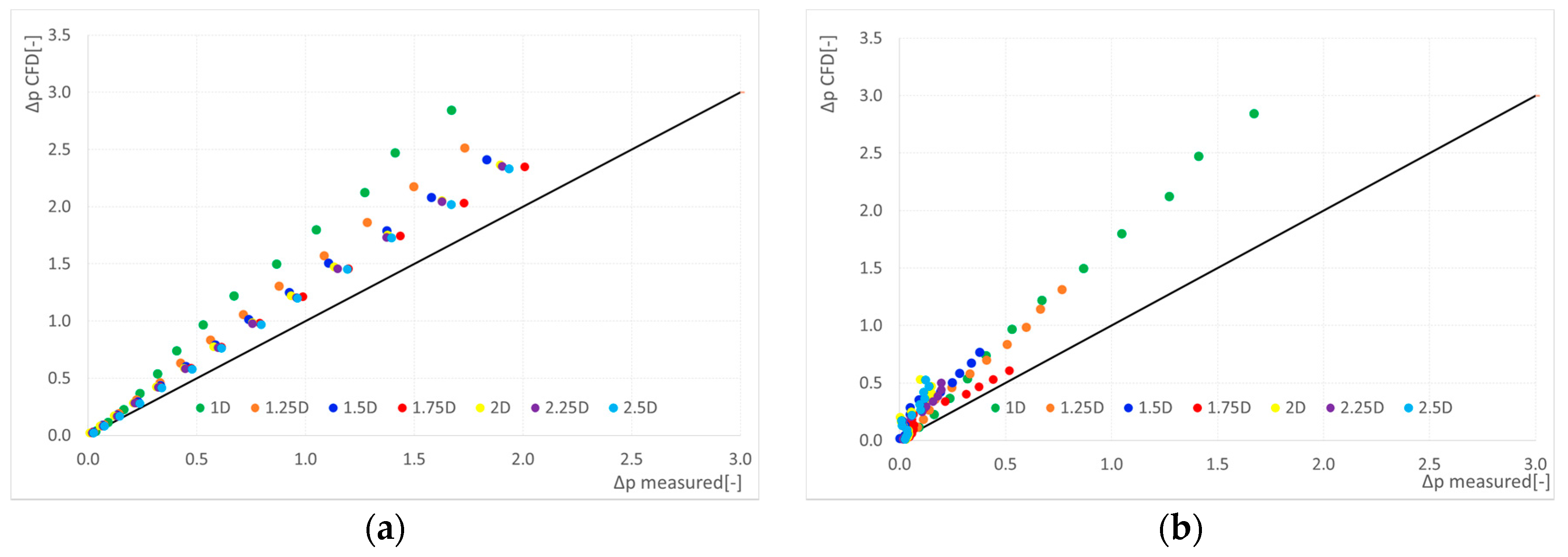
The discrepancy between experimental and numerical results is consistently reduced in CFD analysis 2; however, the trend of the points remains the same and the error increases with flow rate in both CFD analyses. These results illustrate that the CFD software [18] has some limits but, at the same time, we believe it is able to predict the correct trend of pressure losses, thereby allowing for defining the same dependence between pressure losses, flow rate and geometry considered, as can be seen from the numerical−experimental comparison previously presented. Another more robust commercial tool would allow reduction of the error, but would add no surprises to the general considerations we have found. On the other hand, the software used is easy to manage and useful during a first qualitative analysis. In Figure 20, we have plotted the pressure losses obtained from the CFD analysis 1 versus the measured pressure losses (case without cavitation). This was done to analyze the distance between numerical and experimental data. It was found that in the case of single elbow with contraction, with a ratio higher than 1.5, the points are lying approximately near an easy-to-define line with interpolation; in the case of the elbow with expansion, not considering the pressure drop under 0.2 MPa (about 0.3 considering the dimensionless measured pressure drop), for which also the experimental accuracy is quite low, again the points are lying on a line. These considerations make it possible to estimate the error between numerical analysis and the experimental one.

8. Conclusions

This work has focused on the study of pressure losses on manifolds with different methods: Computational Fluid Dynamic (CFD) analysis, semi-empirical approach according to [13], when possible, and experimental characterization. The comparison of the results obtained allows for drawing some guidelines for the design of the manifold channels and to discuss the reliability of CFD analysis as a tool to improve the design of a hydraulic manifold. It was chosen to first focus on simple geometries considering the intersection between the channels of the manifold with one or two 90° elbows. This choice was motivated by the need to compare the results with the ones already published in the literature to validate the analysis and then apply the analysis method to test cases not previously discussed. These cases are the “offset elbow,” the “expansion elbow” and the “contraction elbow”.

Results from CFD simulations show that the virtual analysis can depict the correct trend of pressure drop in all the different geometries analyzed following, at a “certain distance”, the experimental results. The difference between experimental and CFD results normally increases with the flow rate and the pressure drop. The gap is, however, quite high and always with an overestimation of CFD simulations compared with the experimental results; this overestimation can also be found in [12,13], for example.

Going into the detail of manifold design rules, some considerations can be highlighted: first of all, when an elbow with a moderate expansion is included in the manifold, it causes a lower pressure drop; moreover, if reverse flow is possible in the same connections, no great change of pressure drop will be observed in comparison to a normal elbow. Hence, an expansion ratio can be adopted for the “preferred” flow direction without having significant damage in the reverse flow.

Offset intersections introduce a higher pressure drop only when the flow area obtained from the channel intersection is strongly reduced; the designer must therefore reduce offset connections during the manifold design.

When two consecutive elbows are necessary in the manifold passage, a U shape is convenient from the point of view of energy saving, while the S shape is the least successful. When the dimensionless distance L/d between the two elbows is about 13, the two elbows are no longer interacting with one another and the total pressure drop in the passage can be considered as the sum of the two pressure drop values.

The next step of this research will be to analyze what happens with more complex but realistic connections on a manifold block, still comparing the CFD analysis and the experimental results, and deepening the study of aeration/cavitation occurrence.