
Stochastic Residential Harmonic Source Modeling for Grid Impact Studies

Abstract
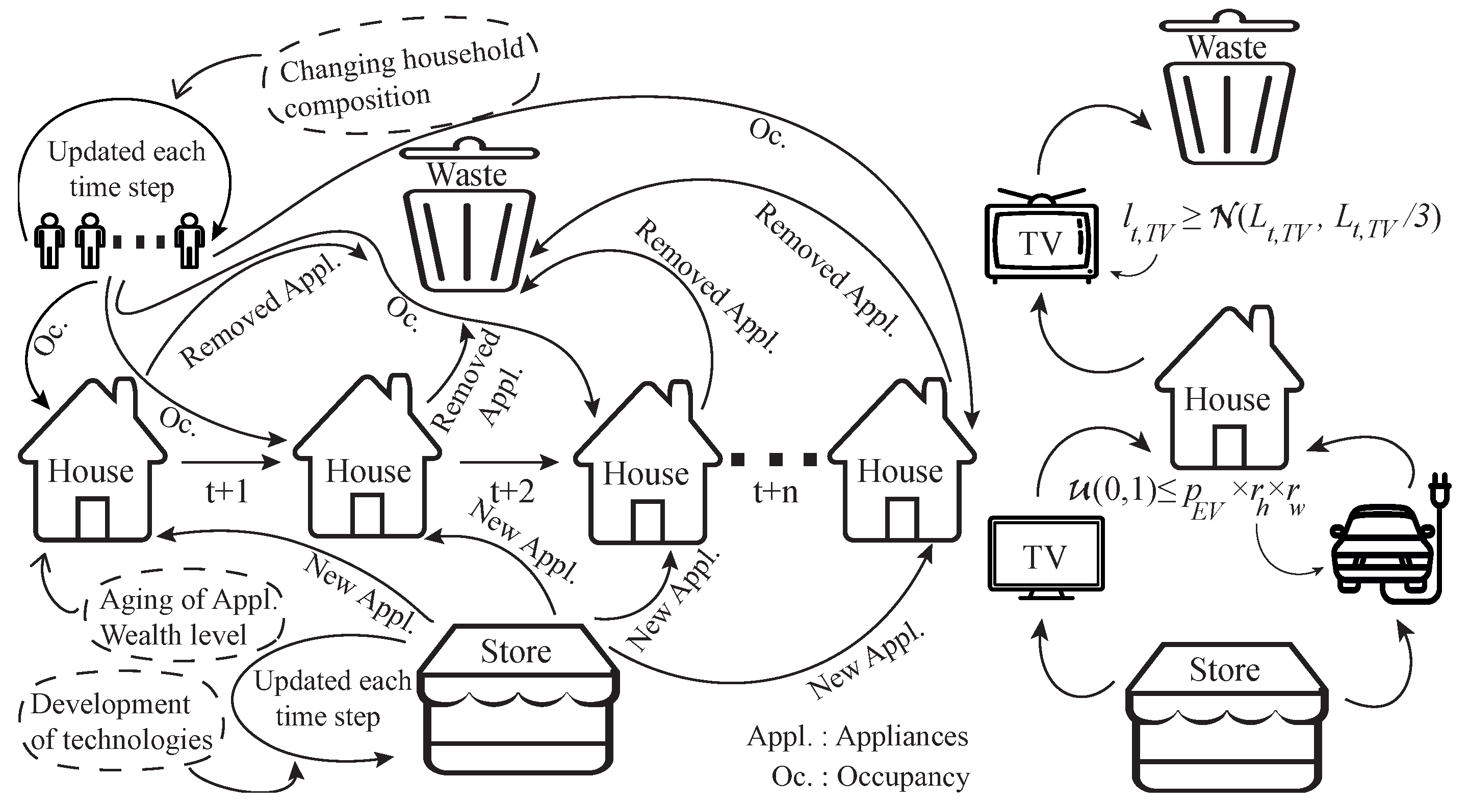
:1. Introduction
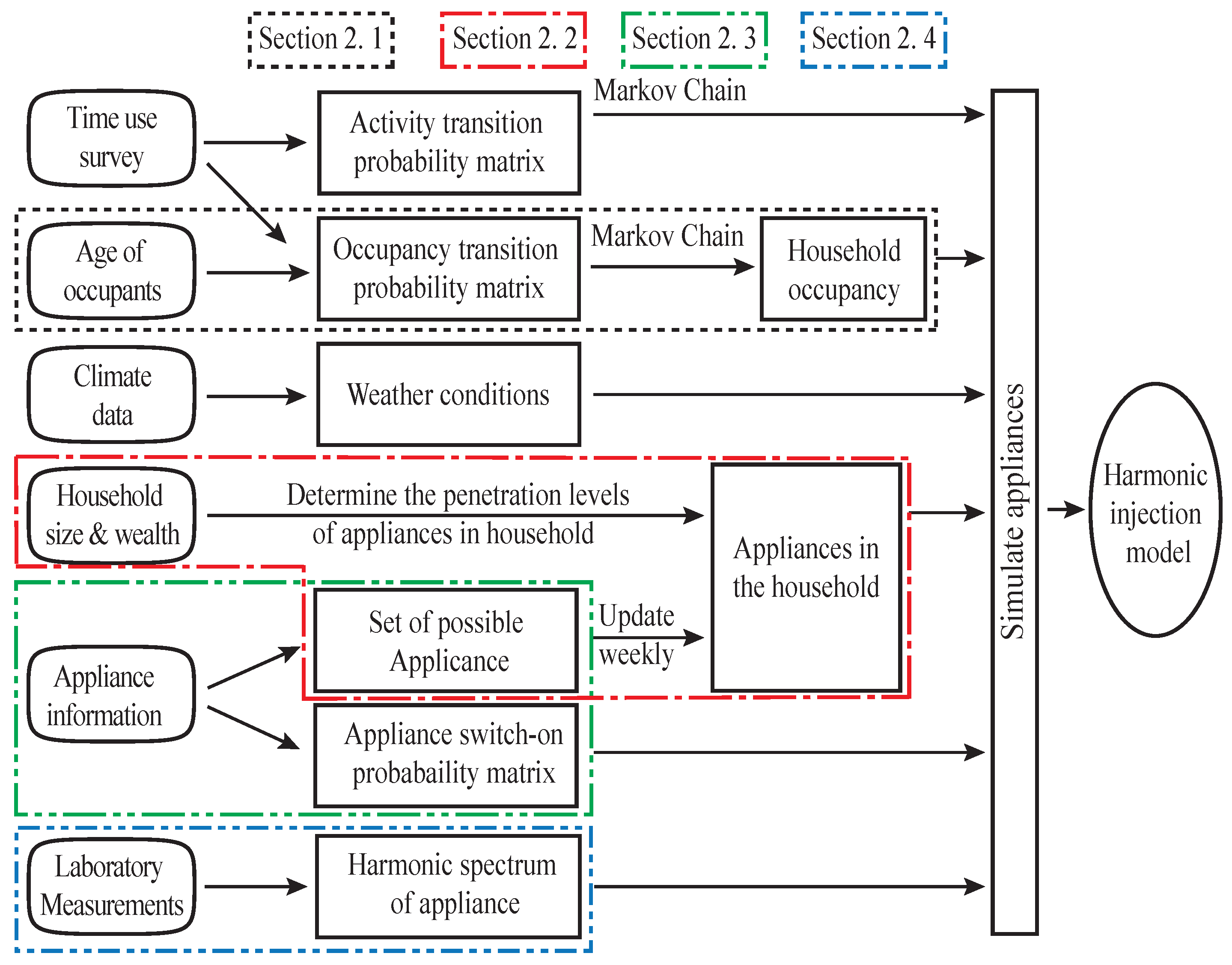
2. Harmonic Injection Modeling
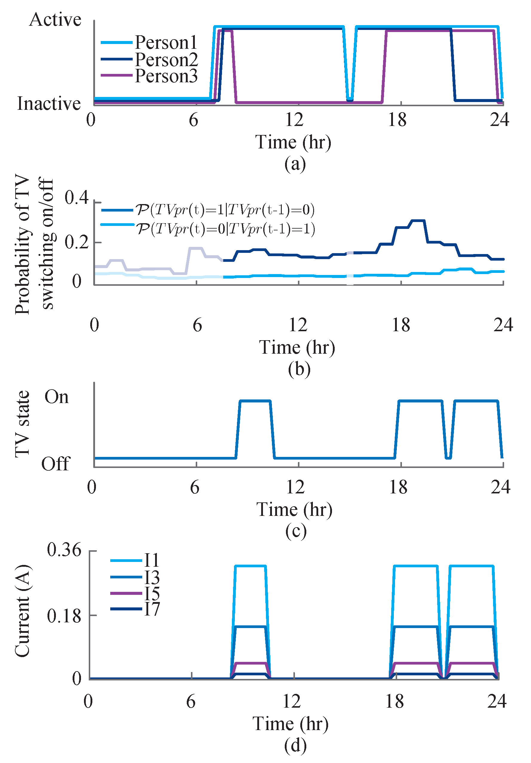
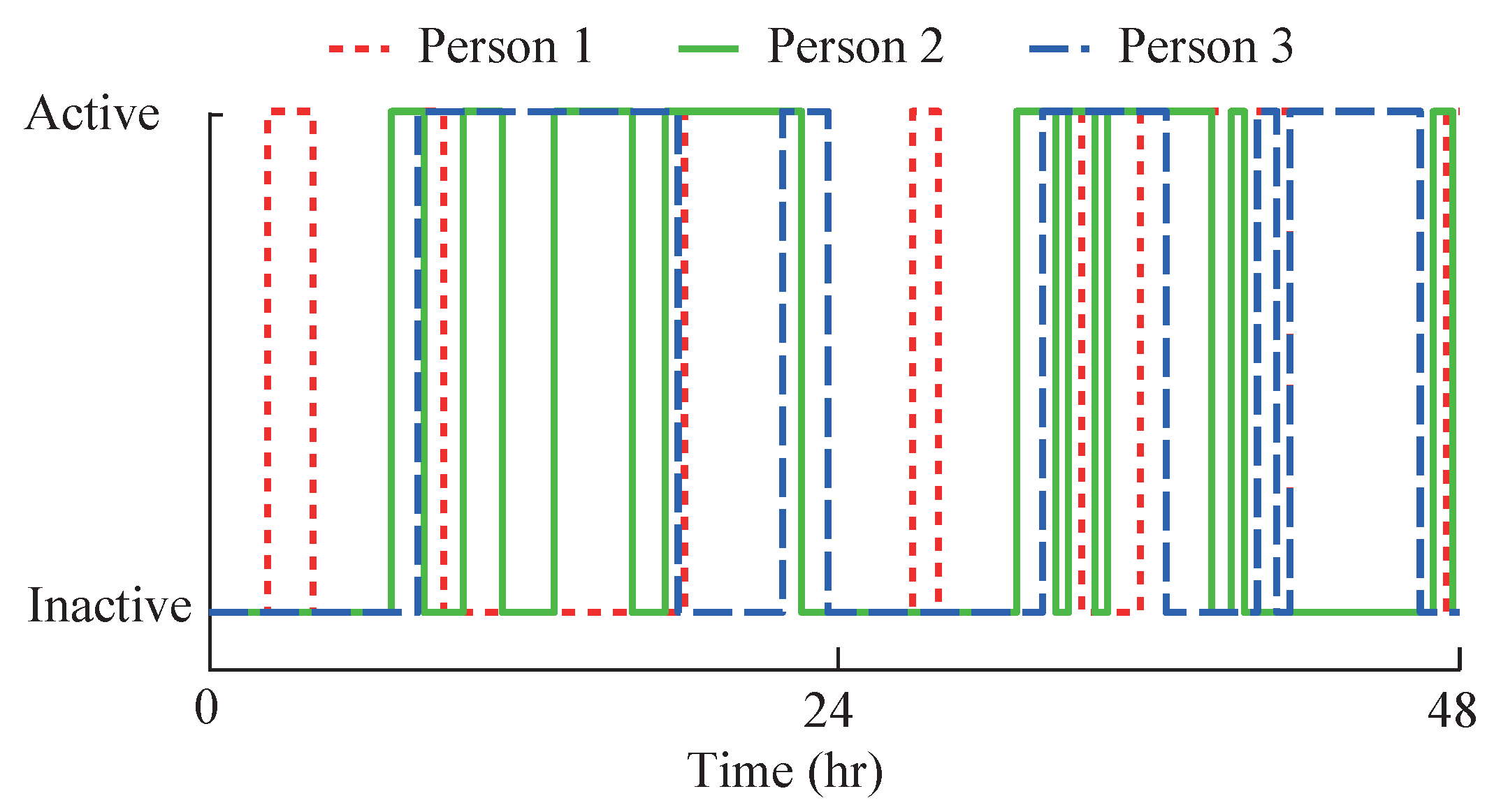
2.1. Occupancy Modeling
2.2. Allocation of Household Appliances
2.3. Appliances Modeling
2.3.1. Base Appliances
2.3.2. Night Appliances
2.3.3. Temperature Adjustment Appliances
2.3.4. Lighting Appliances
2.3.5. Behavioral Appliances
2.3.6. Other Appliances
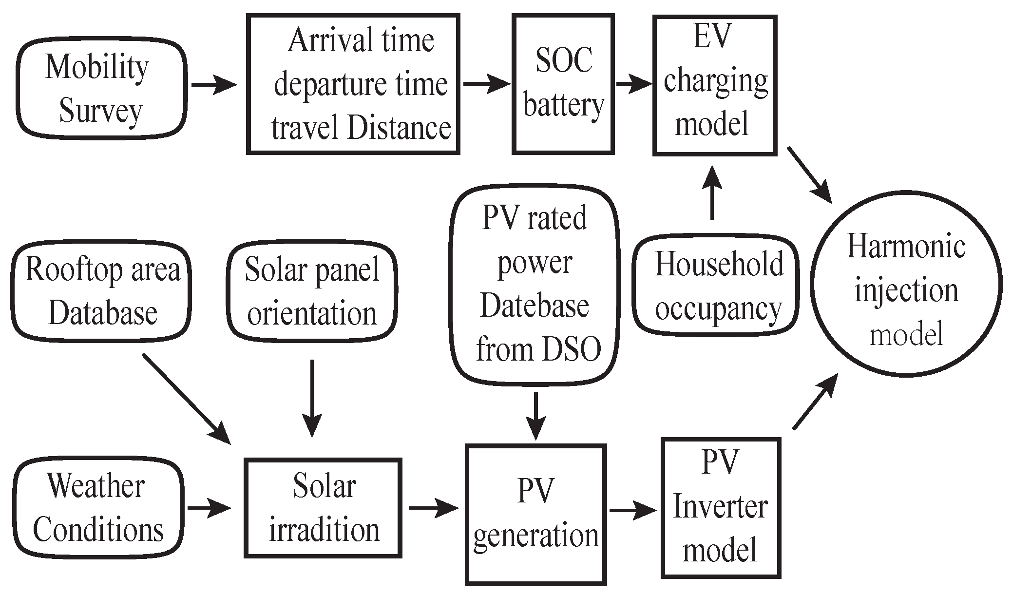
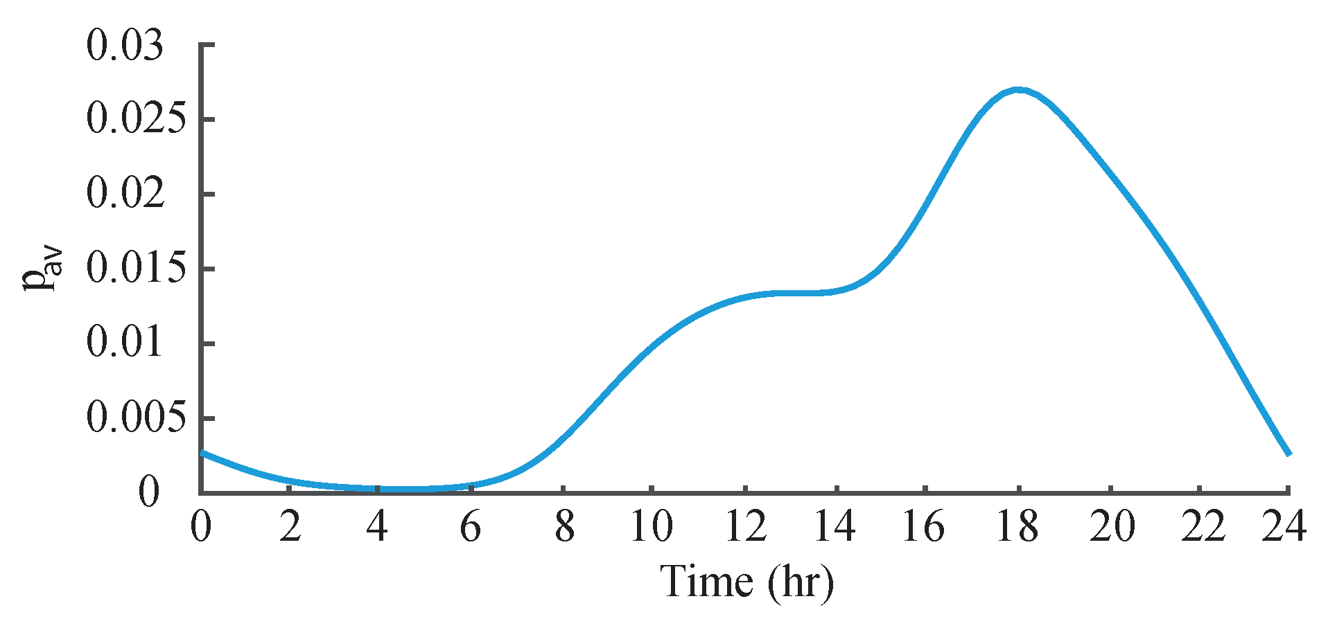
2.3.7. Electric Vehicle
2.3.8. Photovoltaic System
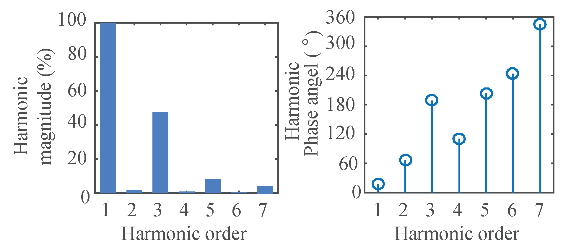
2.4. Harmonic Current Spectra of Appliances
Attenuation and Diversity Effect
2.5. Appliances Power and Harmonic Injection
2.6. Appliance Development Modeling
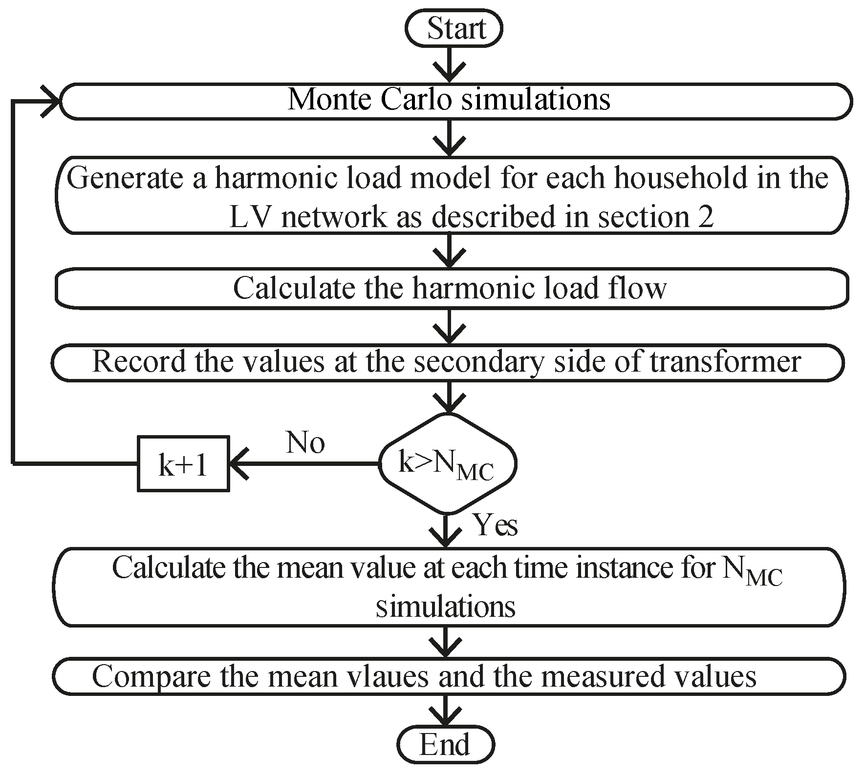
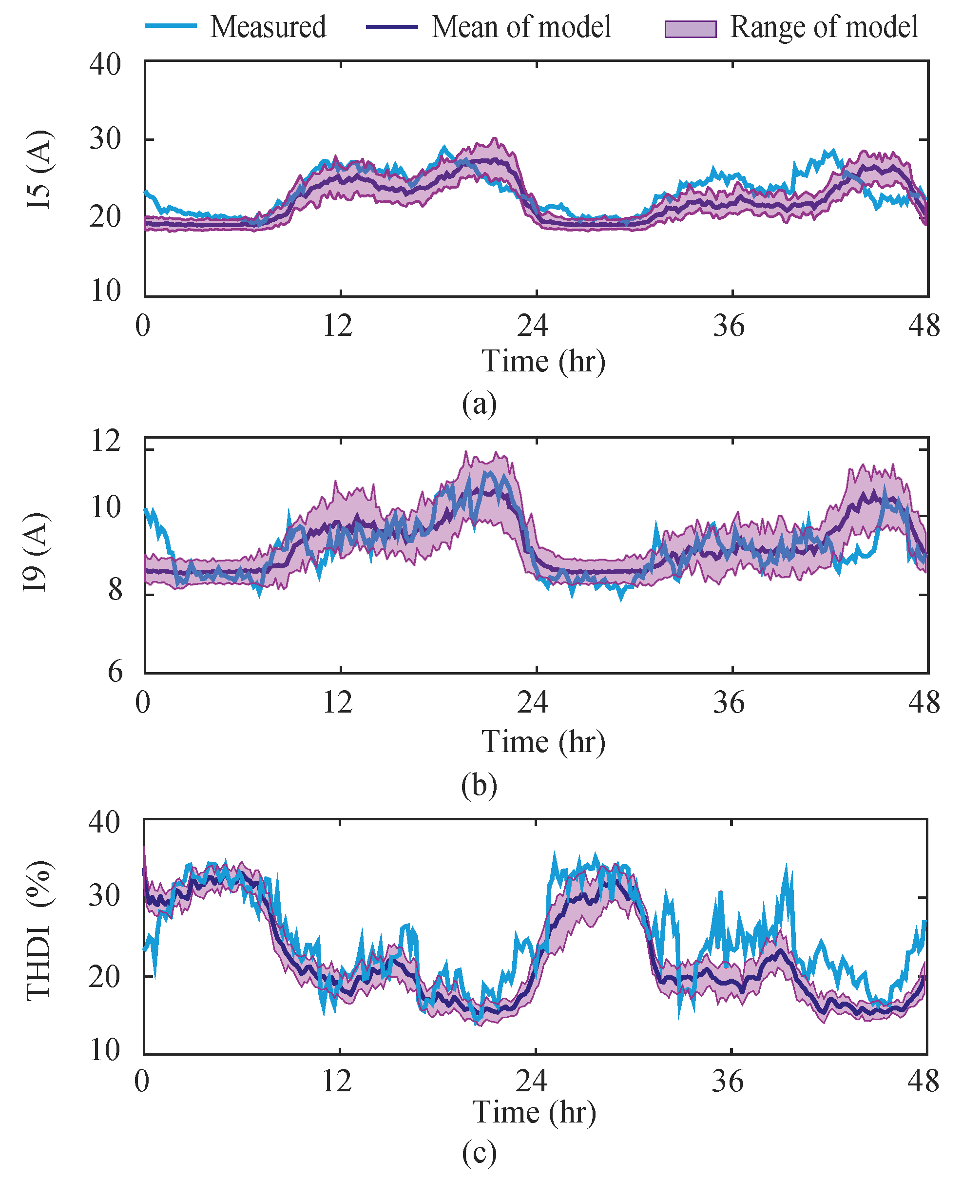
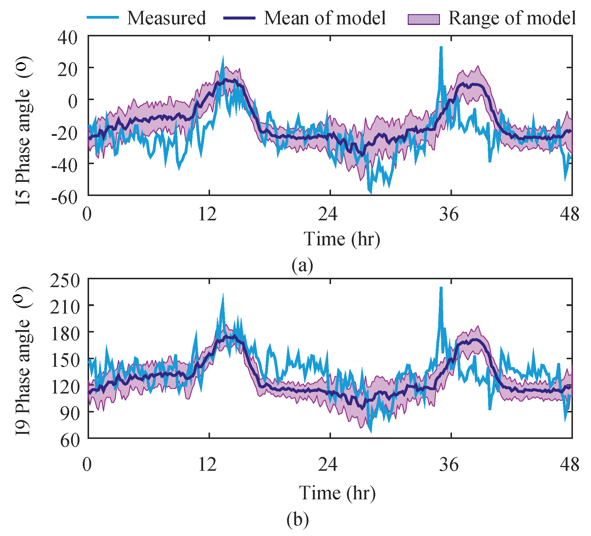
3. Validation of the Harmonic Injection Model
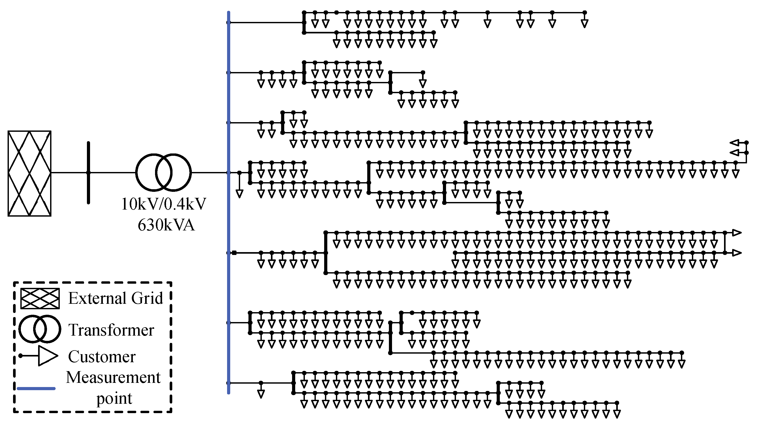
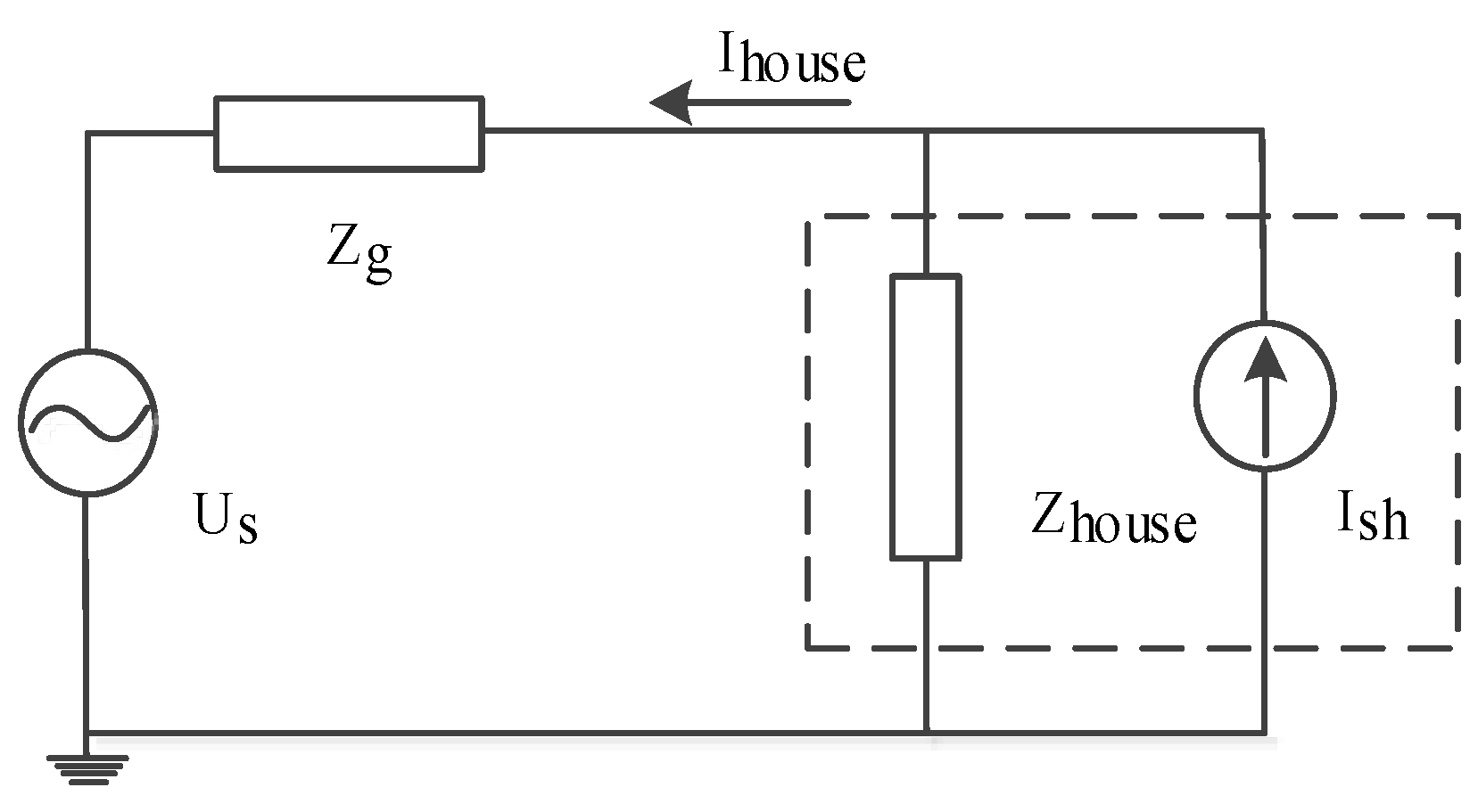
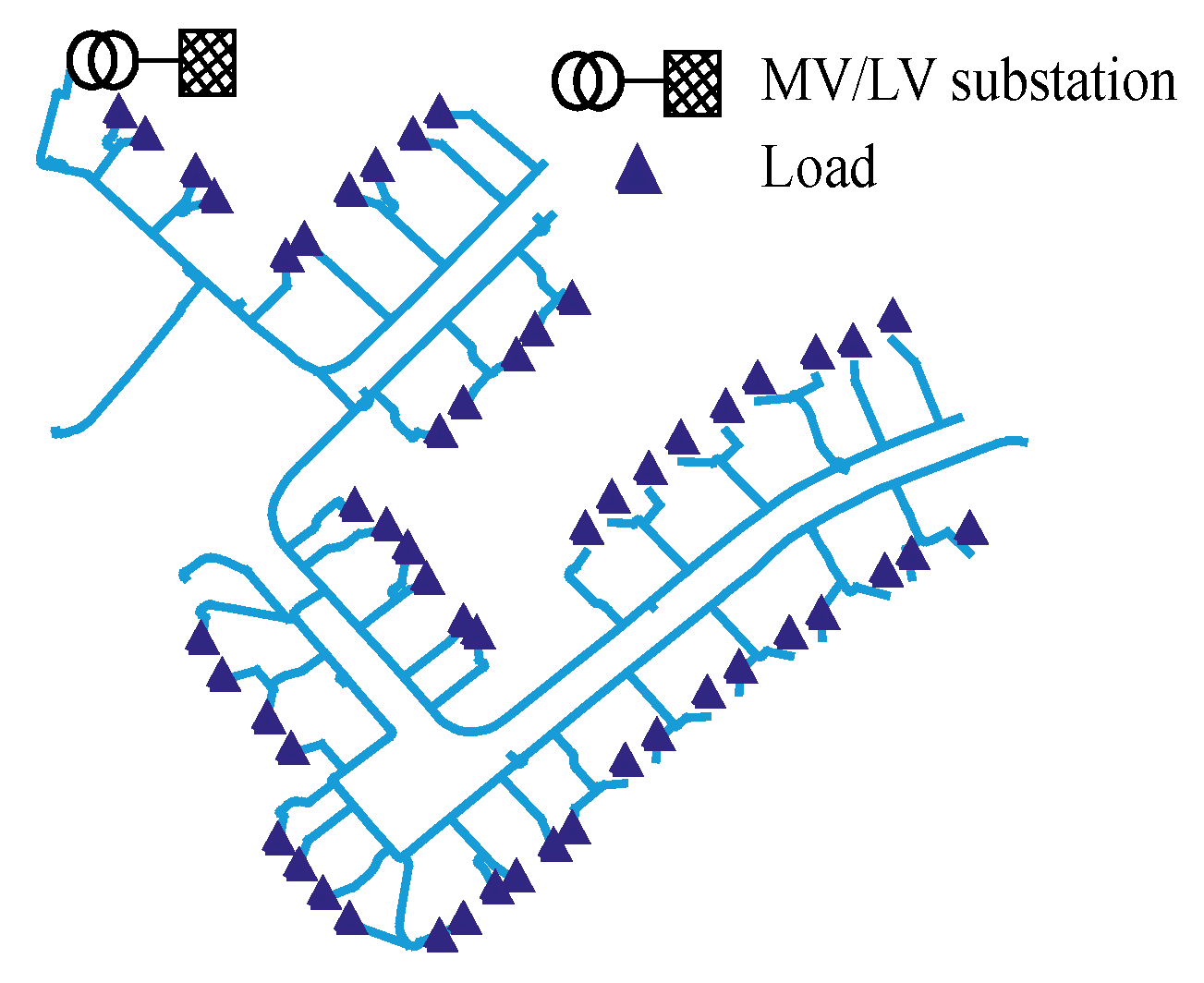
3.1. Residential Network Modeling and Simulation Approach
3.2. Measurement and Simulation Results
4. Case Study
4.1. Scenarios
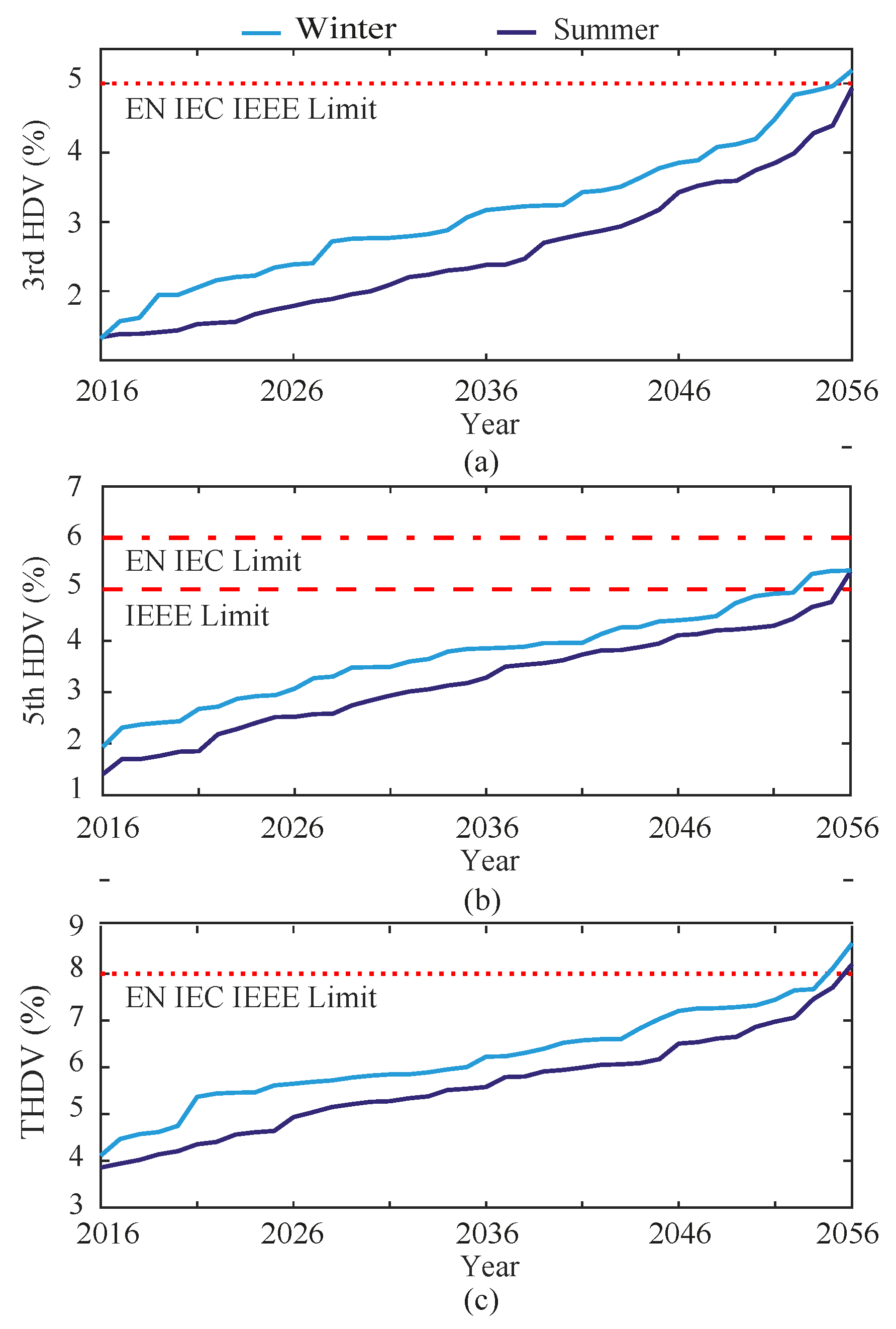
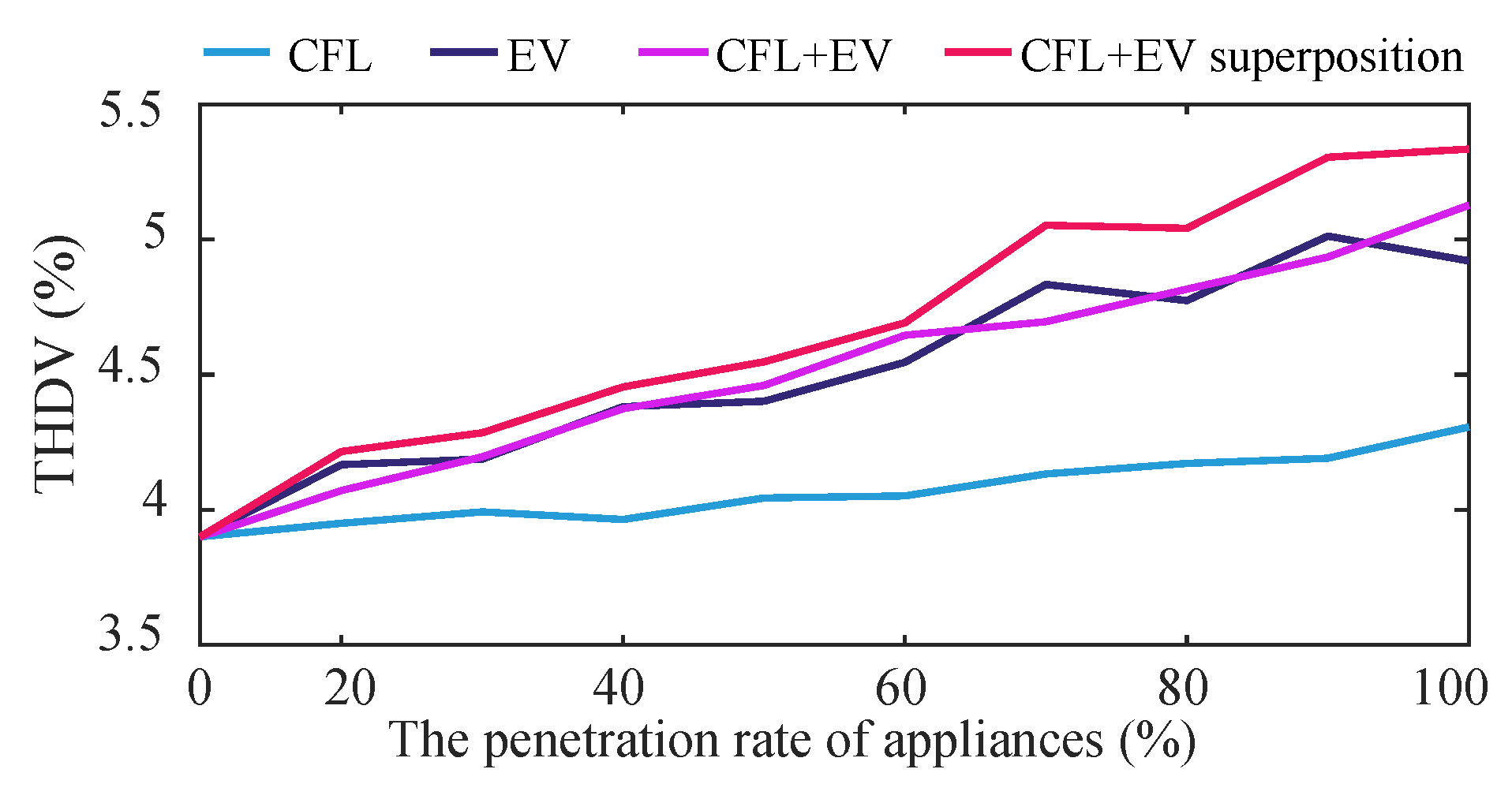
4.2. Harmonic Analysis for Compliance Assessment
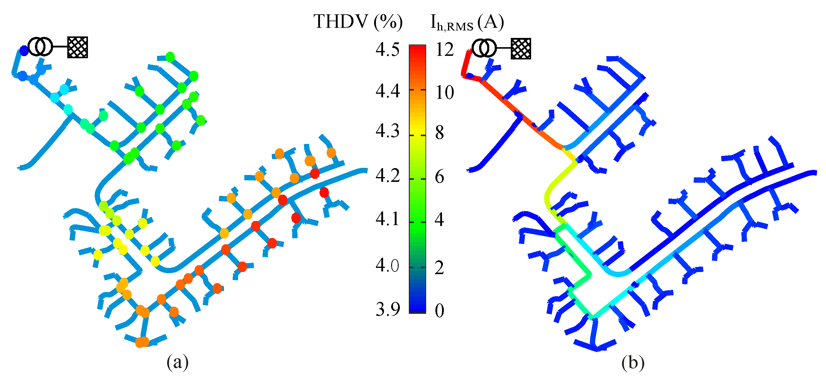
4.3. Harmonic Distortion throughout the Network
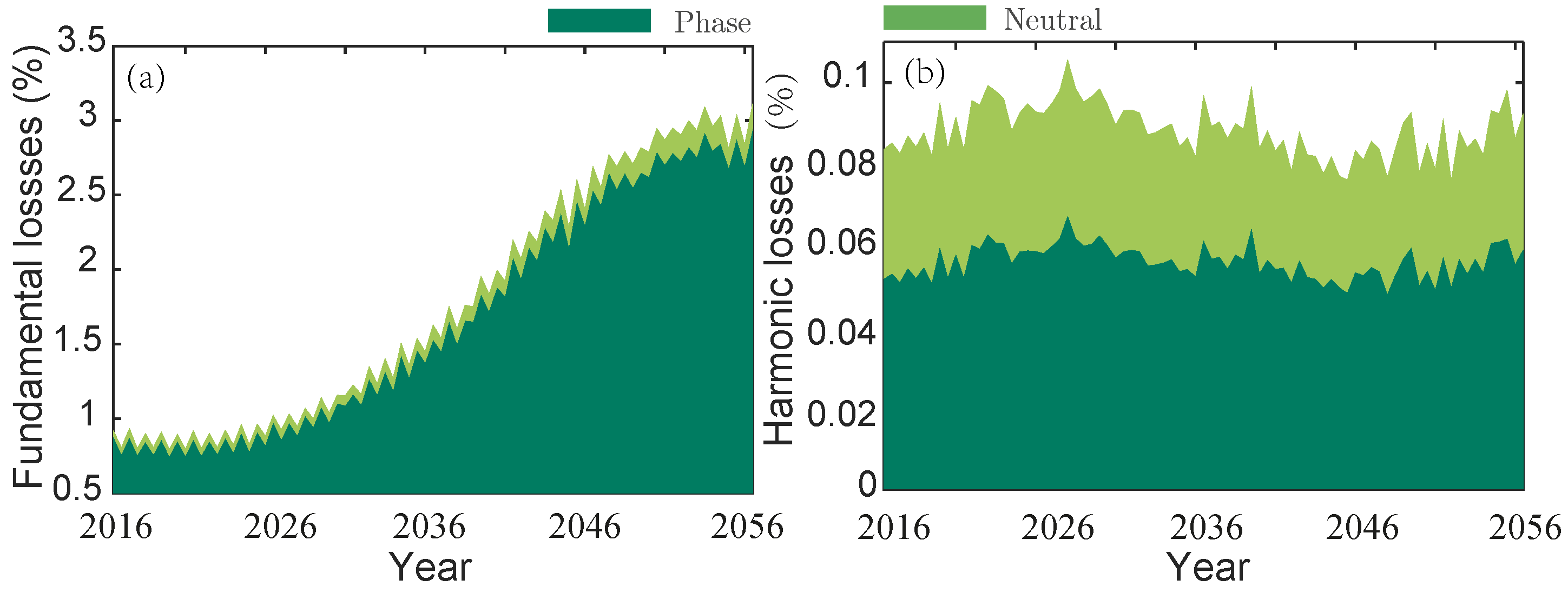
4.4. Losses Due to Harmonic Distortion
4.5. Impact of Specific Appliances
5. Conclusions
Acknowledgments
Author Contributions
Conflicts of Interest
Appendix A

| Category | Appliances |
|---|---|
| Base Appliances | Charger, cordless phone, freezer, modem, refrigerator, water bed. |
| Night Appliances | Dishwasher, electric Boiler, electric blanket. |
| Temperature Adjustment Appliance | air conditioner, electric heater, electric radiator, fan, mechanical ventilation, pumped central heating system, underfloor heating. |
| Lighting Appliances | CFL, incandescent lamp, LED. |
| Behavioral Appliances | Cooker, dryer, DVD player, fryer, iron, laptop, microwave, mixer, oven, personal computer (PC), radio, TV, vacuum cleaner, washing machine. |
| Other Appliances | Coffee machine, drill, electric kettle, hairdryer. |
References
- Watson, N.R.; Scott, T.L.; Hirsch, S.J.J. Implications for distribution networks of high penetration of compact fluorescent lamps. IEEE Trans. Power Deliv. 2009, 24, 1521–1528. [Google Scholar] [CrossRef]
- Dolara, A.; Leva, S. Power quality and harmonic analysis of end user devices. Energies 2012, 5, 5453–5466. [Google Scholar] [CrossRef]
- DeCastro, A.G.; Rönnberg, S.K.; Bollen, M.H.; Moreno-Muñoz, A. Study on harmonic emission of domestic equipment combined with different types of lighting. Int. J. Electr. Power Energy Syst. 2014, 55, 116–127. [Google Scholar]
- Patsalides, M.; Stavrou, A.; Efthymiou, V.; Georghiou, G.E. Towards the establishment of maximum pv generation limits due to power quality constraints. Int. J. Electr. Power Energy Syst. 2012, 42, 285–298. [Google Scholar] [CrossRef]
- Zhou, N.C.; Lou, X.X.; Yu, D.; Wang, Q.G.; Wang, J.J. Harmonic injection-based power fluctuation control of three-phase pv systems under unbalanced grid voltage conditions. Energies 2015, 8, 1390–1405. [Google Scholar] [CrossRef]
- Orr, J.A.; Emanuel, A.E.; Pileggi, D.J. Current harmonics, voltage distortion, and powers associated with electric vehicle battery chargers distributed on the residential power system. IEEE Trans. Ind. Appl. 1984, IA-20, 727–734. [Google Scholar] [CrossRef]
- Jiang, C.; Torquato, R.; Salles, D.; Xu, W. Method to assess the power-quality impact of plug-in electric vehicles. IEEE Trans. Power Deliv. 2014, 29, 958–965. [Google Scholar] [CrossRef]
- Sharma, H.; Rylander, M.; Dorr, D. Grid impacts due to increased penetration of newer harmonic sources. IEEE Trans. Ind. Appl. 2016, 52, 99–104. [Google Scholar] [CrossRef]
- Collin, A.J.; Tsagarakis, G.; Kiprakis, A.E.; McLaughlin, S. Development of low-voltage load models for the residential load sector. IEEE Trans. Power Syst. 2014, 29, 2180–2188. [Google Scholar] [CrossRef]
- Nijhuis, M.; Gibescu, M.; Cobben, J. Bottom-up markov chain monte carlo approach for scenario based residential load modeling with publicly available data. Energy Build. 2016, 112, 121–129. [Google Scholar] [CrossRef]
- Salles, D.; Jiang, C.; Xu, W.; Freitas, W.; Mazin, H.E. Assessing the collective harmonic impact of modern residential loads—Part I: Methodology. IEEE Trans. Power Deliv. 2012, 27, 1937–1946. [Google Scholar] [CrossRef]
- Flett, G.; Kelly, N. An occupant-differentiated, higher-order markov chain method for prediction of domestic occupancy. Energy Build. 2016, 125, 219–230. [Google Scholar] [CrossRef] [Green Version]
- Druckman, A.; Sinclair, P.; Jackson, T. A geographically and socio-economically disaggregated local household consumption model for the UK. J. Clean. Prod. 2008, 16, 870–880. [Google Scholar] [CrossRef] [Green Version]
- PANDA. Equipment Harmonic Database. Technische Universitlit Dresden. Available online: http://www.panda.et.tu-dresden.de/ (accessed on 16 September 2016).
- Bonner, A.; Grebe, T.; Gunther, E.; Hopkins, L.; Marz, M.B.; Mahseredjian, J.; Miller, N.W.; Ortmeyer, T.H.; Rajagopalan, V.; Ranade, S.; et al. Modeling and simulation of the propagation of harmonics in electric power networks. I. Concepts, models, and simulation techniques. IEEE Trans. Power Deliv. 1996, 11, 452–465. [Google Scholar]
- Sociaal en Cultureel Planbureau (SCP) and Centraal Bureau voor de Statistiek (CBS). Tijdsbestedingsonderzoek 2011—TBO 2011. Available online: http://dx.doi.org/10.17026/dans-x4m-rew4 (accessed on 7 June 2016).
- Brooks, S.; Gelman, A.; Jones, G.L.; Meng, X.L. (Eds.) Handbook of Markov chain Monte Carlo; Chapman and Hall/CRC: Boca Raton, FL, USA, 2011.
- Nederlands Instituut Voor Budgetvoorlichting. Energielastenbeschouwing: Verschillen in Energielasten Tussen Huishoudens Nader Onderzocht; NIBUD: Utrecht, The Netherlands, 2009. [Google Scholar]
- Fazeli, R.; Ruth, M.; Davidsdottir, B. Temperature response functions for residential energy demand: A review of models. Urban Clim. 2016, 15, 45–59. [Google Scholar] [CrossRef]
- Richardson, I.; Thomson, M.; Infield, D.; Delahunty, A. Domestic lighting: A high-resolution energy demand model. Energy Build. 2009, 41, 781–789. [Google Scholar] [CrossRef] [Green Version]
- Stokes, M.; Rylatt, M.; Lomas, K. A simple model of domestic lighting demand. Energy Build. 2004, 36, 103–116. [Google Scholar] [CrossRef]
- Verzijlbergh, R.A.; Grond, M.O.W.; Lukszo, Z.; Slootweg, J.G.; Ilic, M.D. Network impacts and cost savings of controlled EV charging. IEEE Trans. Smart Grid 2012, 3, 1203–1212. [Google Scholar] [CrossRef]
- Verzijlbergh, R.A. Thepower of Electric Vehicles—Exploring the Value of Flexible Electricity Demand in a Multi-Actor Context. Ph.D. Thesis, Delft University of Technology, Delft, The Netherlands, 2013. [Google Scholar]
- Verzijlbergh, R.A.; Lukszo, Z.; Ilić, M.D. Comparing different EV charging strategies in liberalized power systems. In Proceedings of the 2012 9th International Conference on the European Energy Market, Florence, Italy, 10–12 May 2012; pp. 1–8.
- Wiginton, L.; Nguyen, H.; Pearce, J. Quantifying rooftop solar photovoltaic potential for regional renewable energy policy. Comput. Environ. Urban Syst. 2010, 34, 345–357. [Google Scholar] [CrossRef]
- Gouws, R.; Lukhwareni, T. Factors influencing the performance and efficiency of solar water pumping systems: A review. Int. J. Phys. Sci. 2012, 7, 6169–6180. [Google Scholar]
- Khoo, Y.S.; Nobre, A.; Malhotra, R.; Yang, D.; Rüther, R.; Reindl, T.; Aberle, A.G. Optimal orientation and tilt angle for maximizing in-plane solar irradiation for PV applications in singapore. IEEE J. Photovolt. 2014, 4, 647–653. [Google Scholar] [CrossRef]
- Benghanem, M. Optimization of tilt angle for solar panel: Case study for Madinah, Saudi Arabia. Appl. Energy 2011, 88, 1427–1433. [Google Scholar] [CrossRef]
- Bhattacharyya, S. Power Quality Requirements and Responsibilities at The Point of Connection. Ph.D. Thesis, Eindhoven Univertsity of Technology, Eindhoven, The Netherlands, 2011. [Google Scholar]
- Ahmed, E.E.; Xu, W.; Zhang, G. Analyzing systems with distributed harmonic sources including the attenuation and diversity effects. IEEE Trans. Power Deliv. 2005, 20, 2602–2612. [Google Scholar] [CrossRef]
- EN 50160: Voltage Characteristics in Public Distribution Systems; Copper Development Association: New York, NY, USA, 2004.
- Ye, G. Investigation on Low Voltage Network and Future Development Based on Field Measurements. Master’s Thesis, Eindhoven University of Technology, Eindhoven, The Netherlands, 2013. [Google Scholar]
- Thunberg, E.; Soder, L. A norton approach to distribution network modeling for harmonic studies. IEEE Trans. Power Deliv. 1999, 14, 272–277. [Google Scholar] [CrossRef]
- IEEE PES Distribution System Analysis Subcommittee’s Distribution Test Feeder Working Group, 2016. Available online: ewh.ieee.org/soc/pes/dsacom/testfeeders/index.html (accessed on 4 October 2016).
- Ministry of Transport, Public Works and Water Management. Mobiliteitsonderzoek Nederland; Ministry of Transport, Public Works and Water Management: Hague, The Netherlands, 2009. (In Dutch)
- Koninklijk Nederlands Meteorologisch Instituut. Uurgegevens Van Het Weer in Nederland. Available online: http://projects.knmi.nl/klimatologie/uurgegevens/selectie.cgi (accessed on 21 September 2016).
- Eichhammer, W.; Fleiter, T.; Schlomann, B.; Faberi, S.; Fioretto, M.; Piccioni, N.; Lechtenböhmer, S.; Schüring, A.; Resch, G. Study on the Energy Savings Potentials in EU Member States, Candidate Countries and EEA Countries; Fraunhofer Institute for Systems and Innovation Research: Karlsruhe, Germany, 2009. [Google Scholar]
- Janssen, L.; Okker, V.; Schuur, J. Welvaart en Leefomgeving, een Scenariostudie Voor Nederland in 2040; Centraal Planbureau: Den Haag, The Netherlands, 2006. [Google Scholar]
- Veldman, E. Power Play Impacts of Flexibility in Future Residential Electricity Demand on Distribution Network Utilisation. Ph.D. Thesis, Eindhoven University of Technology, Eindhoven, The Netherlands, 2013. [Google Scholar]
- Variz, A.M.; Niquini, F.M.M.; Pereira, J.L.R.; Barbosa, P.G.; Carneiro, S.; Ribeiro, P.F. Allocation of power harmonic filters using genetic algorithm. In Proceedings of the 2012 IEEE 15th International Conference on Harmonics and Quality of Power (ICHQP), Hong Kong, China, 17–20 June 2012; pp. 143–149.
- Moran, S. A line voltage regulator/conditioner for harmonic-sensitive load isolation. In Proceedings of the Conference Record of the 1989 IEEE Industry Applications Society Annual Meeting, San Diego, CA, USA, 1–5 October 1989; Volume 1, pp. 947–951.


| hth | Fund. | 3rd | 5th | 7th | 9th | 17th | 21th | |
|---|---|---|---|---|---|---|---|---|
| Magnitude (%) | 6.69 | 11.3 | 12.0 | 18.1 | 16.2 | 30.2 | 33.7 | 22.1 |
| Phase angle () | - | 14.4 | 11.3 | 16.7 | 23.8 | 67.5 | 62.0 | - |
© 2017 by the authors. Licensee MDPI, Basel, Switzerland. This article is an open access article distributed under the terms and conditions of the Creative Commons Attribution (CC BY) license ( http://creativecommons.org/licenses/by/4.0/).
Share and Cite
Ye, G.; Nijhuis, M.; Cuk, V.; Cobben, J.F.G. Stochastic Residential Harmonic Source Modeling for Grid Impact Studies. Energies 2017, 10, 372. https://doi.org/10.3390/en10030372
Ye G, Nijhuis M, Cuk V, Cobben JFG. Stochastic Residential Harmonic Source Modeling for Grid Impact Studies. Energies. 2017; 10(3):372. https://doi.org/10.3390/en10030372
Chicago/Turabian StyleYe, Gu, Michiel Nijhuis, Vladimir Cuk, and J.F.G. (Sjef) Cobben. 2017. "Stochastic Residential Harmonic Source Modeling for Grid Impact Studies" Energies 10, no. 3: 372. https://doi.org/10.3390/en10030372