
A Novel Multi-Objective Optimal Approach for Wind Power Interval Prediction


School of Electrical Engineering, Wuhan University, Wuhan 430072, China
*
Author to whom correspondence should be addressed.
Energies 2017, 10(4), 419; https://doi.org/10.3390/en10040419
Submission received: 10 January 2017
/
Revised: 14 March 2017
/
Accepted: 20 March 2017
/
Published: 23 March 2017
(This article belongs to the Special Issue Sustainable Energy Technologies)
Abstract
:Numerous studies on wind power forecasting show that random errors found in the prediction results cause uncertainty in wind power prediction and cannot be solved effectively using conventional point prediction methods. In contrast, interval prediction is gaining increasing attention as an effective approach as it can describe the uncertainty of wind power. A wind power interval forecasting approach is proposed in this article. First, the original wind power series is decomposed into a series of subseries using variational mode decomposition (VMD); second, the prediction model is established through kernel extreme learning machine (KELM). Three indices are taken into account in a novel objective function, and the improved artificial bee colony algorithm (IABC) is used to search for the best wind power intervals. Finally, when compared with other competitive methods, the simulation results show that the proposed approach has much better performance.
1. Introduction
Wind power is rapidly growing due to its clean, renewable characteristics and mature technology. To solve the problems of serious environmental pollution and fossil energy depletion, clean energy will gradually replace fossil energy, and wind power will become increasingly important in the grid. However, its intermittency and uncertainty has brought great challenges to the operation of the grid. Therefore, high-quality wind power prediction is an important means of ensuring the safe and stable operation of the power system.
Much research on wind power prediction methods has been conducted and some of the mainstream wind power forecasting methods and systems along with their practical applications are summarized in Reference [1]. Broadly speaking, the approaches for wind speed and power forecasting can be divided into three categories: physical forecasting approaches, statistical forecasting approaches, and combination approaches [2].
Physical approaches basically deal with the transformation of numerical weather prediction (NWP) data into wind-electric power. They perform well over a longer horizon, but are limited by the accuracy of the NWP data. Statistical approaches generally use historical data to build statistical models that show good performance for short-term forecasts. The combination approach combines different approaches and retains the advantages of each one; however, this is not always better than the best individual forecasts.
Numerous approaches have been proposed for forecasting wind speed and wind power. However, most existing approaches focus on point forecasting, where the prediction errors that exist cause uncertainties to the forecast results. Furthermore, Reference [3] made a comparison of a series of well-known wind power forecasting methods where the accuracy of those methods was found to be less than reported. In addition to point prediction, the uncertainty estimation can provide fluctuation intervals of wind power, which will give a more comprehensive reference to grid dispatchers and operators.
The uncertainty prediction of wind power can be divided into three categories, i.e., probabilistic forecasts, risk indices, and scenarios of generation. In recent years, probabilistic forecasting has received much attention; however, the conventional methods of probabilistic forecast often require special prior assumptions of error distribution [4]. It was found that the probability density function of forecast errors varied greatly in Reference [5], which means that it is not reasonable to assume a specific distribution of the forecast errors. Quantile regression [6], the kernel density forecast method [7], and the Gaussian process [8,9] were used to present probabilistic wind power prediction intervals (PIs) without any assumption; however, the construction methods of PIs require complex mathematical calculations or rely on results from point forecasting. An upper and lower bound estimation (LUBE) approach that uses the prediction interval coverage probability (PICP) and the prediction interval normalized average width (PINAW) to evaluate the PIs was proposed in Reference [10]. However, it was proved in Reference [11] that the coverage width-based criterion (CWC) score used in Reference [10] did not have suitable properties in which to evaluate the PIs. Furthermore, the CWC score could not measure the PIs in a comprehensive way as the deviation of the data not covered by the PI was not considered. The interval deviation index was taken into account in the interval score as an additive term to the interval width index in References [12,13], but it was difficult to decide which one was more important given that the interval deviation has a tendency to decrease as the interval width increases. Therefore, three indexes—PICP, PINAW and normalized average deviation (NAD)—were used to evaluate the PIs in this study. In addition, a novel multi-objective function that could satisfy all the criteria was used to construct the optimal PIs.
Moreover, the inherent characteristics of wind power sequences were not considered in the previous methods. To resolve this problem, the wavelet transform [14] and ensemble empirical mode decomposition (EEMD) methods [4] were employed to decompose the original wind power time series into several components, and proved to be superior to the method without decomposition. Variational mode decomposition (VMD) proved to be excellent compared to the EEMD [15] and was adopted in this study.
Neural network was used to obtain PIs in Reference [16], and the extreme learning machine (ELM) employed in Reference [17] was proven to be superior to neural network (NN)-based methods. However, ELM also has some drawbacks, which include difficulties in determining the number of hidden layer nodes, and the lack of consideration of structural risk, which leads to over-fitting. The kernel extreme learning machine (KELM) which is described in Reference [18] was adopted to improve the generalization and stability of the forecasting model, and an improved artificial bee colony algorithm (IABC) was used to optimize the penalty coefficient C and kernel parameter σ of KELM.
In summary, the main contributions of this article are: (1) applying KELM (optimized by IABC) to obtain PIs as KELM has good generalization and stability; and (2) introducing a novel multi-objective function, which provides a powerful authority to the decision-maker for satisfying all the indices.
The rest of this paper is organized as follows. The overall structure and theoretical knowledge of the approach proposed are described in Section 2. The method of constructing optimal PIs is depicted in Section 3, and the simulation results of the proposed approach compared with other methods are presented in Section 4. Finally, conclusions are drawn in Section 5.
2. Proposed Approach for Forecasting Wind Power Intervals
The structure of the proposed approach had two stages (Figure 1). In the first stage, the wind power sequence was decomposed into several subseries using VMD, and the subseries were then grouped into reconstructed components using sample entropy (SE) theory. In the second stage, the optimal wind power PIs were constructed using KELM and IABC. A novel multi-objective function to construct the optimal PIs was also proposed. A description of the hybrid approach is given below.
2.1. Variational Mode Decomposition
Variational mode decomposition is an adaptive signal decomposition method proposed by Dragomiretskiy and Zosso [19]. It is used to decompose the original signal into a series of band-limited modes uk, where the center of each mode is pulsation wk.
The bandwidth of each mode is obtained through the following steps: First, the associated analytic signal of each mode is computed using Hilbert transform to obtain a unilateral frequency spectrum; second, each mode’s frequency spectrum is shifted to baseband by mixing with an exponential tuned to the estimated center frequency; finally, the bandwidth is obtained through the H1 Gaussian smoothness of the demodulated signal. The resulting constrained variational problem is shown as follows:
where, δ is the Dirac distribution, k represents the number of modes, * denotes convolution, and represent the set of all modes and their center frequencies , respectively.
Making use of a quadratic penalty term and Lagrange multipliers, the constrained variational problem can be addressed as follows:
The detailed process is described in Reference [19], and the pseudocode of the VMD method is shown below (Algorithm 1).
where represents the variance of the white noise. The solutions can be expressed as:
where , , and represent the Fourier transforms of , , and , respectively, and n denotes the number of iterations. Based on a large number of simulation tests, the maximum number of iterations n was set as 500.
| Algorithm 1 Process of VMD |
| Initialize , , , |
| repeat |
| for do Update for all : Update : end for Dual ascent for all : |
| until convergence: |
2.2. Sample Entropy
Sample entropy (SE) was used to calculate the complexity of the subseries. The more complex the series, the greater its SE value. The SE value of one series is denoted by , which is defined as the negative logarithm of the conditional probability that two sequences similar for m points remain similar at the next point, excluding self-matches. N is the number of data points, m denotes the embedding dimension, and r denotes the tolerance. The description of the SE technique can be found in Reference [20].
The SE value is related with m and r, but its increase or decrease trend is not affected by m and r for it has a good consistency. Generally, the value of m is 2, and r equals 0.1–0.25 SD in which SD is the standard deviation of the time series.
2.3. Kernel Extreme Learning Machine
To improve the generalization and stability of ELM, the kernel function was introduced to propose the KELM algorithm. The output function of KELM can be written compactly as follows [18]:
where I is a diagonal matrix, C is the penalty coefficient, T is the matrix of targets, H is the hidden-layer output matrix and kernel matrix is defined as follows:
The hidden layer feature mapping h(x) does not need to be known to users, and the dimensionality L of the feature space (number of hidden nodes) also does not need to be given. However, the performance of KELM is sensitive to the penalty coefficient C and kernel parameter σ; therefore, the Bat-inspired algorithm was used to optimize these two parameters.
2.4. Artificial Bee Colony Algorithm and Its Modification
The artificial bee colony algorithm is an optimization algorithm that was proposed by Karaboga in 2005 and a detailed description of artificial bee colony algorithm (ABC) can be found in Reference [21]. In this paper, the position of each food source represented a solution which contains the values of the penalty coefficient C and the kernel parameter σ for the KELM.
In each iteration, an onlooker bee chooses a food source depending on the probability value defined in Equation (7):
where is the fitness of solution , and S is the number of food sources equal to the number of employed bees or onlooker bees.
The employed bees search for the food source according to Equation (8):
where is a random number; ; in which D is the dimension of the solution space; and k is different from i.
After the evaluation of each candidate source, if the fitness is not improved, then the associated food source is abandoned and the employed bee becomes a scout. The scout discovers a new food source according to Equation (9):
To decrease the possibility of the local optimum, an improved ABC—based on opposition-based learning—was proposed in Reference [22]. The modification strategy can be described as follows:
For each food source, a random value λ was generated and compared with an adaptive variable PM which was defined as , where g and G represent the current number and the maximum number of iterations. If , then opposition-based learning was carried out. Opposition-based learning is depicted below:
3. Construction of Optimal PIs
3.1 Reliability and Sharpness of PIs
Reliability and sharpness are required and desirable properties for evaluating the probabilistic forecast [23]. The PIs are composed of an upper and lower boundary with a certain probability level. PI coverage probability and PI normalized average width [24] are commonly used to describe the reliability and sharpness of the constructed PIs and are defined as follows:
- 1
- Prediction interval coverage probability (PICP)where N denotes the number of prediction points, = 1 when the target value in which Li and Ui are the lower and upper bound of each PI, otherwise = 0.
- 2
- Prediction interval normalized average width (PINAW)where R is the range of the target values and is used to normalize the average width of PIs.PICP is used to describe the reliability of the constructed PIs, and PINAW is used to characterize the sharpness of the PIs. However, these two indices are not enough to evaluate the PIs. For example, when the and of two PIs are the same, the optimal PI cannot be judged if the real data are not covered by the PIs and the deviation from the upper bound (or lower bound) is different. Therefore, the normalized average deviation was introduced in this study.
- 3
- Normalized average deviation (NAD)The NAD is used to express the deviation of the data which are not covered by the PI.where the expression of is as follows:
3.2. The Objective Function of PIs
The optimal PIs with high reliability (i.e., the coverage probability of PIs will be as close to the prescribed nominal level of confidence as possible), narrow average width, and small accumulated deviation are required, which can be expressed as a multi-objective optimization problem. However, these three indices conflict with each other, for example, when the PICP increases, the PINAW increases correspondingly; when the NAD decreases, the PICP usually tends to increase.
It is not possible to simply translate a multi-objective optimization problem into a single-objective solution as the multiple objects are incommensurable (without uniform metrics between targets, it is difficult to directly compare the targets) and conflict with each other. Therefore, a Pareto-based method was proposed in this paper to construct a multi-objective model, which could overcome the random selection of target weights and the difficulty in dealing with objects with different dimensions. The concrete method of constructing the multi-objective model is as follows.
For the convenience of solution, the problem of making close to the corresponding PI nominal confidence (PINC) is transformed into the minimization problem of coverage probability error through Equation (15):
Generally, a smaller indicates more reliable PIs. As the PIs with a low confidence level are meaningless, a 90% confidence level was required in this study. Therefore, the multi-objective optimization model was established as follows:
where is the output weight of the KELM and is optimized by IABC. The proposed multi-objective optimization method was based on the Pareto theory, which is depicted below [25,26].
The Pareto optimum solution set is a solution set that provides a set of alternatives for decision-makers for flexible choice. In the Pareto optimum solution set, there is no solution that is definitely better than another, and it can be explained by dominant and non-dominant concepts. For example, X1 and X2 are assumed as the resultant solutions, and the objective functions are f1, f2, and f3. If f1(X1) < f1(X2) and f2(X1) < f2(X2) and f3(X1) < f3(X2), then X1 dominates X2; if f1(X1) > f1(X2) and f2(X1) > f2(X2) and f3(X1) > f3(X2), then X2 dominates X1. Otherwise, X1 and X2 do not dominate each other, and they are called non-dominant solutions, which create the Pareto optimum solution set. Thus, selecting a solution from the Pareto optimum solution set provides great flexibility. The relative optimal solution was chosen through the technique for order preference by similarity to an ideal solution (TOPSIS) [27].
3.3. Prediction Process
The flowchart of the proposed approach for constructing PIs using KELM optimized by IABC is shown in Figure 2, and the detailed steps are as follows.
Step 1: Input the training data, validation data, testing data, and the initial parameters of the KELM and IABC. The output data of the training set is processed as per Equation (17) to form the initial output intervals of the training set:
where is the original output, is the processed output interval, and R is a random number of the interval [0, 1].
Step 2: Produce the initial population. Apply the KELM with initial parameters to the training set to obtain the weighting factor , which is then applied to the validation data.
Step 3: Compare the real data and the PIs obtained from the validation set, and calculate the indices based on Equations (11)–(15) to form the objective functions according to Section 3.2.
Step 4: Put the solutions of all food sources into the Pareto optimal solution set and delete the dominant solutions.
Step 5: In each iteration, make use of the IABC to optimize the parameters of the KELM, calculate the objective functions using the PIs obtained from the validation set, and update the Pareto solution set. Thus, the optimal KELM models can be obtained.
Step 6: Apply the optimal models to the testing set, choose the relative optimal solution using TOPSIS, and output the results of wind power PIs.
4. Numerical Results and Discussions
To evaluate the performance of the approach proposed in this paper, the approaches using KELM and ELM were compared to prove the superiority of KELM. Next, the approach using the interval score [13] (defined in Equation (18)) was compared with the Pareto-based approach to verify the superiority of the multi-objective function proposed in this paper. In addition, the approach where only two indices (IPICP and IPINAW) were used and the approach using quantile regression were compared with the proposed approach. The detailed simulation results are shown in Section 4.2.
where represents the width of the PI, = 1 − PINC.
4.1. Dataset and Parameter Settings
In the studies, the data used for testing was from two wind farms (i.e., wind farm M and wind farm J) located in northern China and southern China, respectively. The capacity of wind farm M is 50 MW, and the data was recorded in 15 min interval. The capacity of wind farm J is 95 MW, and the data was recorded in 5 min interval. Taking the data of one month as an example, the data were divided into three groups of training samples, validation samples and testing samples at a proportion of 60%, 20% and 20%, respectively.
Regarding the VMD algorithm, the number k of modes should be assigned in advance. It is shown that too few modes result in the incomplete decomposition of the signal, and too many modes may lead to over-decomposition or extra noise. The optimal mode number can be selected using the difference between the center frequencies of the subseries S(k) and S(k − 1), as the center frequency is closely related to the decomposition results of VMD [28]. By decomposing the historical wind power series, it was found that the value of Δf tended to be stable when the value of k was from one to nine. Furthermore, the simulation results showed that number of subseries in the EEMD process was nine. Thus, the number of modes was set as nine. The other parameters in the VMD process were set as per Reference [29]. The penalty factor α and the tolerance of the convergence criterion ε were set to default values of 2000 and 10-6, respectively.
The size of the IABC population was set as 30 as per Reference [22], and the iteration number was set as 100 based on the fact that the IABC convergences after 100 iterations based on many experiments.
4.2. Numerical Results and Analysis
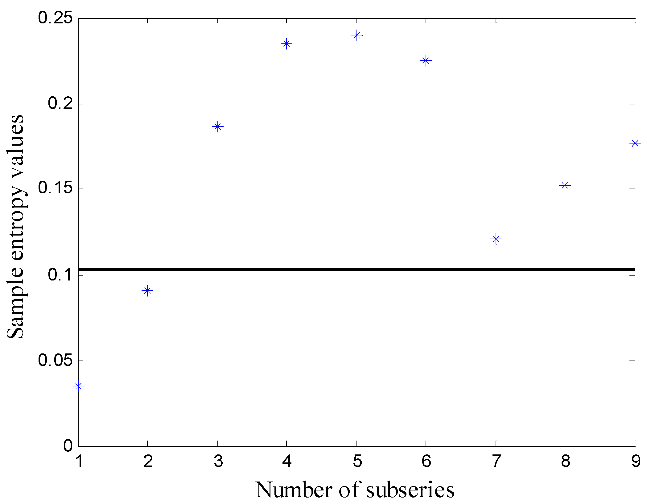
The original wind power time series of one month was decomposed using VMD. Next, the SE of every subseries was calculated and is shown in Figure 3. The solid line in Figure 3 represents the sample entropy of the original series.
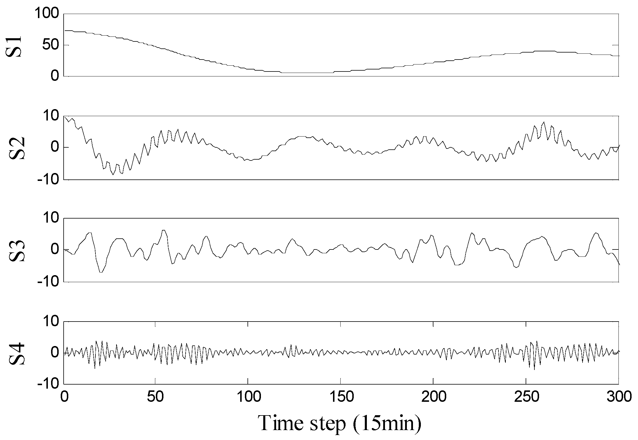
Next, the subseries were reconstructed according to the following rules: the subseries with SE values smaller than the original series were added (i.e., subseries 1 and 2 in Figure 3), the subseries with SE values bigger than the original series and close to each other with a distance smaller than 0.05 were combined (i.e., the third and ninth subseries were combined, the fourth to sixth subseries were combined, and the seventh and eighth subseries were combined). After processing, the reconstructed subseries are shown in Figure 4. For clarity, only a portion of the data (the first 300 points) are shown.
It can be seen in Figure 4 that the reconstructed subseries have obvious regularity, where the frequency increases from top to bottom, and each subseries has periodicity to a certain extent. For each subseries, the method described in Section 3.3 was used for interval prediction and the forecasting results are shown in Figure 5. For clarity, only a portion of the data (the first 200 points) are shown.
It can be seen in Figure 5 that most of the real values are within the PIs, indicating that the proposed approach is effective. The detailed values of the indices can be seen in Table 1.
4.2.1. Comparison of KELM and ELM
To evaluate the performance of the KELM, the interval prediction methods using KELM and ELM are compared in this section. The simulations of these two approaches were conducted 10 times using the historical data in July from wind farm M, and the results are shown in Table 1. The mean value and standard deviation for each index are also provided in Table 1.
Table 1 shows that the PICP of the KELM is closer to the PINC than that of the ELM and the PINAW of KELM is narrower, except the NAD is slightly bigger, indicating that the method using the KELM has a better performance. Another significant point deduced from Table 1 is that the method based on the KELM is more stable as the standard deviations of the KELM are much smaller than those of the ELM.
4.2.2. Analysis of Forecasting Results
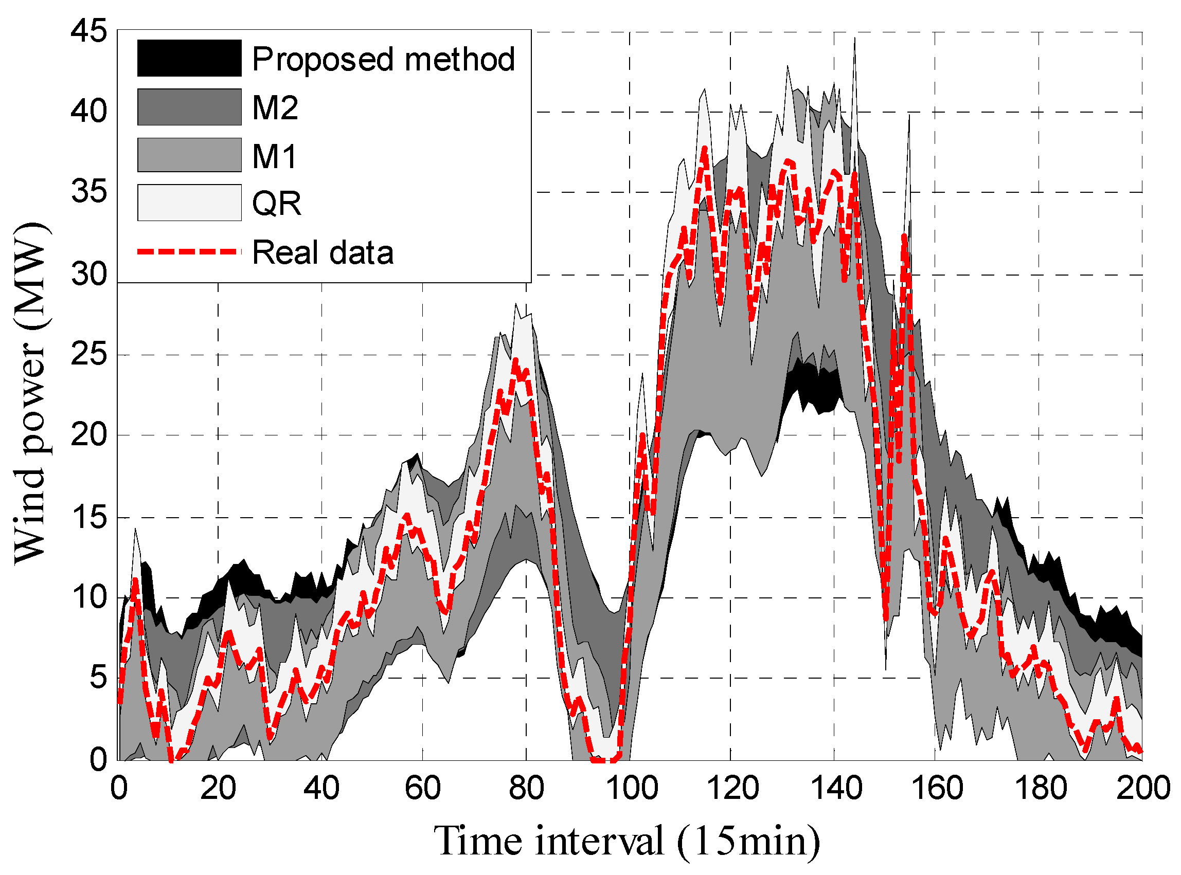
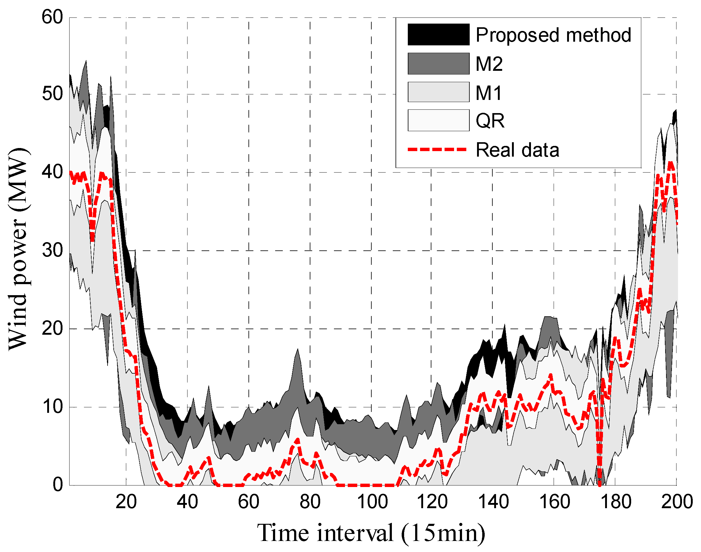
For further validation of the superiority of the interval prediction method proposed in this paper, the results of the approach which used the multi-objective function based on interval scores (abbreviated as M1) are given in Table 2. Furthermore, the results of the approach based on the multi-objective function (where only two indices (IPICP and IPINAW) were used) and those of the approach using quantile regression (abbreviated as M2 and QR, respectively) are shown for comparison with the proposed approach. PIs with PINC 90% obtained by the proposed approach and the other methods in two different months are displayed in Figure 6 and Figure 7.
It can be seen in Figure 6 and Figure 7 that the real data of the wind power are mostly covered by the constructed PIs, which indicates the effectiveness of these methods. The detailed indices of these methods are shown in Table 2. The mean values (Mean) and average coverage probability errors (ACPE) are also given in Table 2.
The following conclusions can be drawn from Table 2:
- 1
- In terms of the reliability (the closer the PICP is to the PINC, the better), almost all the predicted results of the proposed method, M1 and M2 are closer to 90% than the results of QR. The maximum values of the proposed method, M1, M2 and QR are 92.5%, 92.54%, 92.65% and 100%, respectively, and the minimum values of the proposed method, M1, M2 and QR are 88.25%, 87.5%, 87.54% and 82.72%, respectively. The ACPE values of the proposed method, M1, M2 and QR are 1.514, 1.56, 1.531 and 6.209, respectively, indicating that the overall reliability of the proposed method is comparable to that of M1 or M2, and the performance of the proposed method is slightly better than the other two methods. It can also be deduced that the QR approach has the worst performance as its ACPE value is the biggest.
- 2
- In terms of the PINAW (the smaller the better), the maximum, mean and minimum values of the proposed method are 0.284, 0.217 and 0.116, respectively; the maximum, mean and minimum values of M1 are 0.328, 0.251 and 0.148, respectively; the maximum, mean and minimum values of EEMD are 0.291, 0.225 and 0.132, respectively. From the overall level of view, the proposed method performs the best.
- 3
- In terms of the NAD (the smaller the better), the maximum, mean and minimum values of the proposed method are 0.093, 0.026 and 0.002, respectively; the maximum, mean and minimum values of M1 are 0.187, 0.084 and 0.005, respectively; the maximum, mean and minimum values of M2 are 0.192, 0.11 and 0.035, respectively. It can be concluded that the overall performance of the proposed method is superior to the others.
As seen in Table 2, across all months, the proposed method outperforms the other approaches with the resultant ACPE closer to zero, which indicates the high reliability of the constructed PIs. In addition, at the same level of reliability, the proposed method outperforms other approaches with narrower PINAWs and smaller NADs. Thus, it can be deduced that the overall performance of the proposed multi-objective function performs better than other approaches in constructing PIs.
To verify the stability of the proposed method, another set of experiments based on the data in different seasons from wind farm J were conducted, and the PIs with three different forecasting horizons (i.e., one step ahead, two steps ahead and three steps ahead) were constructed. The results are shown in Table 3, Table 4 and Table 5, and the same conclusions can be drawn using the same analytical method.
For intuitive observation, the statistical indices of the proposed method, which proved to be better than M1 and M2 based on Table 2, Table 3, Table 4 and Table 5, are shown in Table 6, where PPM>M1 represents the proportion of the proposed method’s results better than M1, PPM>M2 represents the proportion of the proposed method’s results better than M2, and PPM>QR represents the proportion of the proposed method’s results better than QR.
From Table 6, it can be seen that the performance of the proposed method is worse than QR in terms of IPINAW and INAD, but the reliability of the proposed method is much better than QR. Furthermore, most of the proposed method’s indices are better than the other approaches, which indicates the stability and superiority of the proposed approach.
5. Conclusions
Numerous studies regarding wind power prediction indicate that prediction errors exist inevitably and are of great randomness, which causes a certain degree of uncertainty in the prediction results. Therefore, an interval prediction approach was presented in this paper to solve this issue. From a comparison with the simulation results of the other competitive approaches, the following conclusions could be drawn: (1) the KELM performed better than the ELM in wind power interval prediction; (2) the performance of the proposed method was better than that of M1, M2 and QR, which meant that the approach based on the Pareto objective function constructed in this paper was more effective than the other competitive methods; and (3) the results of the QR were worse than those of the other methods, which indicates that the proposed optimal approach performed better than the quantile regression method used for wind power interval forecasting.
Author Contributions
Mengyue Hu carried out the main research tasks and wrote the full manuscript; Zhijian Hu conceived and designed the experiment; Jingpeng Yue organized and processed the data; Menglin Zhang performed the experiments; and Meiyu Hu analyzed the results.
Conflicts of Interest
The authors declare no conflict of interest.
References
- Monteiro, C.; Keko, H.; Bessa, R.; Miranda, V.; Botterud, A.; Wang, J.; Conzelmann, G.; Porto, I. A Quick Guide to Wind Power Forecating: State-of-the-Art 2009, Technical report, Argonne National Laboratory. Available online: http://www.dis.anl.gov/pubs/65614.pdf (accessed on 9 January 2017).
- Jung, J.; Broadwater, R.P. Current status and future advances for wind speed and power forecasting. Renew. Sustain. Energy Rev. 2014, 31, 762–777. [Google Scholar] [CrossRef]
- Croonenbroeck, C.; Ambach, D. A selection of time series models for short- to medium-term wind power forecasting. J. Wind Eng. Ind. Aerodyn. 2015, 136, 201–210. [Google Scholar] [CrossRef]
- Zhang, G.; Wu, Y.; Wong, K.P.; Xu, Z.; Dong, Z.Y.; Iu, H.H. An advanced approach for construction of optimal wind power prediction intervals. IEEE Trans. Power Syst. 2015, 30, 2706–2715. [Google Scholar] [CrossRef]
- Hodge, B.M.; Milligan, M. Wind power forecasting error distributions over multiple timescales. In Proceedings of the IEEE Power and Energy Society General Meeting, Detroit, MI, USA, 24–29 July 2011. [Google Scholar]
- Haque, A.U.; Nehrir, M.H.; Mandal, P. A hybrid intelligent model for deterministic and quantile regression approach for probabilistic wind power forecasting. IEEE Trans. Power Syst. 2014, 29, 1663–1672. [Google Scholar] [CrossRef]
- Bessa, R.J.; Miranda, V.; Botterud, A.; Zhou, Z.; Wang, J. Time-adaptive quantile-copula for wind power probabilistic forecasting. Renew. Energy 2012, 40, 29–39. [Google Scholar] [CrossRef]
- Kou, P.; Gao, F.; Guan, X.; Wu, J. Prediction Intervals for wind power forecasting: Using sparse warped gaussian process. In Proceedings of the IEEE Power and Energy Society General Meeting, San Diego, CA, USA, 22–26 July 2012. [Google Scholar]
- Yan, J.; Li, K.; Bai, E.; Deng, J.; Foley, A.M. Hybrid Probabilistic Wind Power Forecasting Using Temporally Local Gaussian Process. IEEE Trans. Sustain. Energy 2015, 7, 1–9. [Google Scholar] [CrossRef]
- Khosravi, A.; Nahavandi, S.; Creighton, D. A neural network-GARCH-based method for construction of Prediction Intervals. Electr. Power Syst. Res. 2013, 96, 185–193. [Google Scholar] [CrossRef]
- Pinson, P.; Tastu, J. Discussion of “Prediction intervals for short-term wind farm generation forecasts” and “Combined nonparametric prediction intervals for wind power generation”. IEEE Trans. Sustain. Energy 2014, 5, 1019–1020. [Google Scholar] [CrossRef]
- Gneiting, T.; Raftery, A.E. Strictly Proper Scoring Rules, Prediction, and Estimation. J. Am. Stat. Assoc. 2007, 102, 359–378. [Google Scholar] [CrossRef]
- Wan, C.; Xu, Z.; Pinson, P.; Dong, Z.Y.; Wong, K.P. Optimal Prediction Intervals of Wind Power Generation. IEEE Trans. Power Syst. 2014, 29, 1166–1174. [Google Scholar] [CrossRef]
- Hou, Z.J.; Etingov, P.V.; Makarov, Y.V.; Samaan, N.A. Uncertainty Reduction in Power Generation Forecast Using Coupled Wavelet-ARIMA. In Proceedings of the IEEE PES General Meeting | Conference & Exposition, National Harbor, MD, USA, 27–31 July 2014. [Google Scholar]
- Zhang, Y.; Liu, K.; Qin, L.; An, X. Deterministic and probabilistic interval prediction for short-term wind power generation based on variational mode decomposition and machine learning methods. Energy Convers. Manag. 2016, 112, 208–219. [Google Scholar] [CrossRef]
- Quan, H.; Srinivasan, D.; Khosravi, A. Short-term load and wind power forecasting using neural network-based prediction intervals. IEEE Trans. Neural Netw. Learn. Syst. 2014, 25, 303–315. [Google Scholar] [CrossRef] [PubMed]
- Wan, C.; Xu, Z.; Pinson, P.; Dong, Z.Y.; Wong, K.P. Probabilistic forecasting of wind power generation using extreme learning machine. IEEE Trans. Power Syst. 2014, 29, 1033–1044. [Google Scholar] [CrossRef]
- Huang, G.B. An Insight into Extreme Learning Machines: Random Neurons, Random Features and Kernels. Cogn. Comput. 2014, 6, 376–390. [Google Scholar] [CrossRef]
- Dragomiretskiy, K.; Zosso, D. Variational mode decomposition. IEEE Trans. Signal Process. 2014, 62, 531–544. [Google Scholar] [CrossRef]
- Jiang, Y.; Mao, D.; Xu, Y. A fast algorithm for computing sample entropy. Adv. Adapt. Data Anal. 2011, 03, 167–186. [Google Scholar] [CrossRef]
- Karaboga, D.; Basturk, B. On the performance of artificial bee colony (ABC) algorithm. Appl. Soft Comput. 2008, 8, 687–697. [Google Scholar] [CrossRef]
- Bi, X.; Wang, Y. An improved artificial bee colony algorithm. In Proceedings of the International Conference on Computer Research and Development, Shanghai, China, 11–13 March 2011; pp. 174–177. [Google Scholar]
- Pinson, P.; Nielsen, H.A.; Møller, J.K.; Madsen, H.; Kariniotakis, G.N. Non-parametric probabilistic forecasts of wind power: Required properties and evaluation. Wind Energy 2007, 10, 497–516. [Google Scholar] [CrossRef]
- Kavousi-Fard, A.; Khosravi, A.; Nahavandi, S. A new fuzzy-based combined prediction interval for wind power forecasting. IEEE Trans. Power Syst. 2015, 31, 18–26. [Google Scholar] [CrossRef]
- Wan, C.; Niu, M.; Song, Y.; Xu, Z. Pareto optimal prediction intervals of electricity price. IEEE Trans. Power Syst. 2016, 32, 817–819. [Google Scholar] [CrossRef]
- Asrari, A.; Lotfifard, S.; Payam, M.S. Pareto dominance-based multiobjective optimization method for distribution network reconfiguration. IEEE Trans. Smart Grid 2015, 7, 1401–1410. [Google Scholar] [CrossRef]
- Chen, W. On the Problem and Elimination of Rank Reversal in the Application of TOPSIS Method. Oper. Res. Manag. Sci. 2005, 14, 39–43. [Google Scholar]
- Huang, N.; Yuan, C.; Cai, G.; Xing, E. Hybrid Short Term Wind Speed Forecasting Using Variational Mode Decomposition and a Weighted Regularized Extreme Learning Machine. Energies 2016, 9, 989. [Google Scholar] [CrossRef]
- Sun, G.; Chen, T.; Wei, Z.; Sun, Y.; Zang, H.; Chen, S. A Carbon Price Forecasting Model Based on Variational Mode Decomposition and Spiking Neural Networks. Energies 2016, 9, 54. [Google Scholar] [CrossRef]
Figure 1.
Structure of the approach for wind power interval prediction.
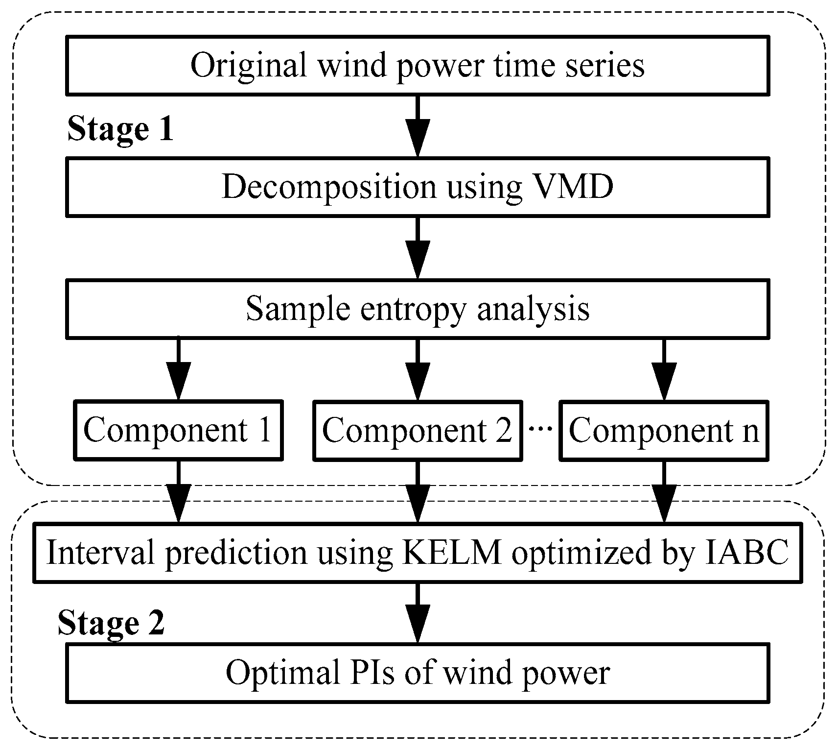
Figure 2.
Flowchart of the prediction approach using KELM-IABC.
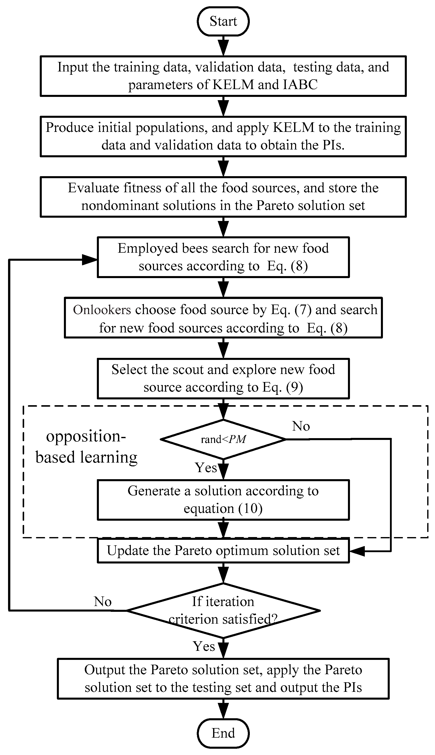
Figure 3.
Distribution of sample entropy values of subseries.

Figure 4.
Distribution of the reconstructed subseries.

Figure 5.
Distribution of wind power prediction intervals (PIs) results with PINC 90%.
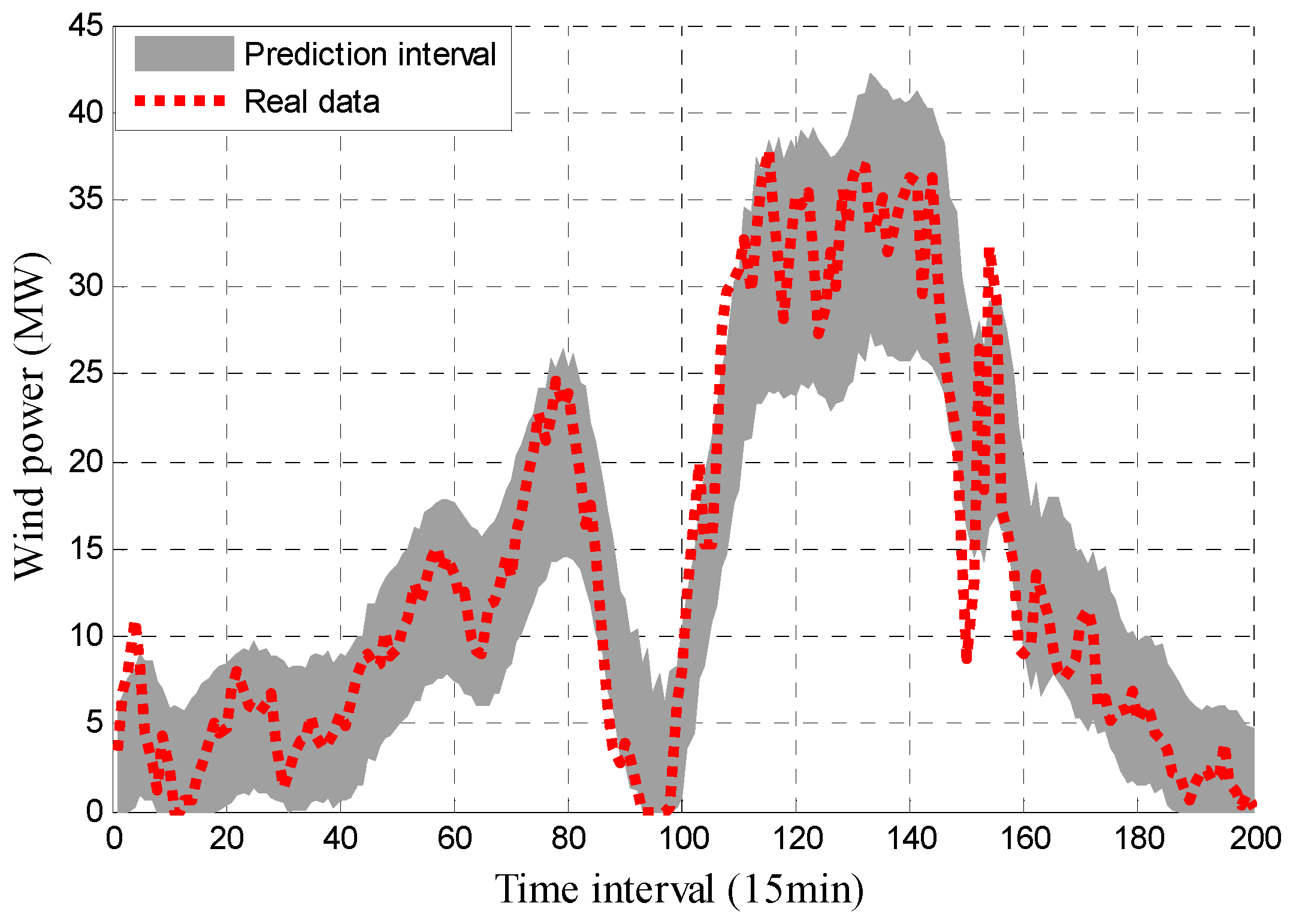
Figure 6.
Distribution of wind power PIs results with PINC 90% in March 2013 of wind farm M.

Figure 7.
Distribution of wind power PIs results with PINC 90% in July 2013 of wind farm M.

Table 1.
Prediction results of interval prediction method using ELM and KELM.
| Number | ELM | KELM | ||||
|---|---|---|---|---|---|---|
| IPICP | IPINAW | INAD | IPICP | IPINAW | INAD | |
| 1 | 92 | 0.195 | 0.188 | 89.5 | 0.164 | 0.187 |
| 2 | 91.5 | 0.188 | 0.191 | 90.25 | 0.152 | 0.175 |
| 3 | 94.25 | 0.208 | 0.178 | 90.75 | 0.171 | 0.183 |
| 4 | 91.25 | 0.194 | 0.193 | 91.75 | 0.191 | 0.176 |
| 5 | 97.25 | 0.245 | 0.111 | 90.5 | 0.166 | 0.182 |
| 6 | 99 | 0.208 | 0.196 | 91.25 | 0.165 | 0.187 |
| 7 | 96.25 | 0.199 | 0.187 | 89.75 | 0.169 | 0.132 |
| 8 | 99.75 | 0.247 | 0.006 | 92 | 0.161 | 0.187 |
| 9 | 91.25 | 0.198 | 0.187 | 91.5 | 0.195 | 0.171 |
| 10 | 92.25 | 0.21 | 0.178 | 91.75 | 0.171 | 0.179 |
| Mean | 94.475 | 0.209 | 0.1615 | 90.9 | 0.171 | 0.176 |
| Std | 3.332 | 0.021 | 0.06 | 0.883 | 0.013 | 0.016 |
Table 2.
Prediction results of wind farm M in different months.
| Month | QR | M1 | M2 | Proposed Method | ||||||||
|---|---|---|---|---|---|---|---|---|---|---|---|---|
| IPICP | IPINAW | INAD | IPICP | IPINAW | INAD | IPICP | IPINAW | INAD | IPICP | IPINAW | INAD | |
| Jan. | 98.23 | 0.083 | 0.005 | 89.75 | 0.161 | 0.086 | 90.71 | 0.181 | 0.062 | 91.25 | 0.193 | 0.048 |
| Feb. | 96.75 | 0.115 | 0.011 | 92.23 | 0.271 | 0.086 | 92.5 | 0.251 | 0.192 | 88.36 | 0.25 | 0.002 |
| Mar. | 100 | 0.121 | 0 | 89.15 | 0.283 | 0.155 | 90.58 | 0.232 | 0.038 | 90.5 | 0.223 | 0.021 |
| Apr. | 82.72 | 0.079 | 0.002 | 91.52 | 0.19 | 0.061 | 87.54 | 0.179 | 0.13 | 91.75 | 0.154 | 0.003 |
| May | 79.75 | 0.101 | 0.001 | 88.75 | 0.26 | 0.187 | 88.3 | 0.215 | 0.101 | 88.25 | 0.216 | 0.012 |
| Jun. | 87.28 | 0.072 | 0.02 | 92.54 | 0.148 | 0.042 | 92.65 | 0.132 | 0.179 | 92.25 | 0.116 | 0.093 |
| Jul. | 90 | 0.086 | 0.049 | 89.35 | 0.209 | 0.022 | 89.5 | 0.221 | 0.161 | 90.5 | 0.205 | 0.02 |
| Aug. | 99 | 0.137 | 0 | 92.33 | 0.328 | 0.005 | 91.97 | 0.291 | 0.035 | 91.75 | 0.284 | 0.003 |
| Sep. | 98.74 | 0.135 | 0 | 88.25 | 0.322 | 0.147 | 91.95 | 0.233 | 0.15 | 91.78 | 0.223 | 0.042 |
| Oct. | 95.25 | 0.095 | 0.003 | 88.73 | 0.235 | 0.057 | 88.75 | 0.227 | 0.065 | 90.25 | 0.214 | 0.009 |
| Nov. | 92.76 | 0.149 | 0.033 | 87.5 | 0.276 | 0.107 | 89.26 | 0.259 | 0.057 | 92.5 | 0.249 | 0.05 |
| Dec. | 93.53 | 0.151 | 0.072 | 91.58 | 0.324 | 0.049 | 88.64 | 0.275 | 0.154 | 92.25 | 0.272 | 0.011 |
| Mean | 92.834 | 0.11 | 0.016 | 90.14 | 0.251 | 0.084 | 90.196 | 0.225 | 0.11 | 90.949 | 0.217 | 0.026 |
| ACPE | 6.209 | / | / | 1.56 | / | / | 1.531 | / | / | 1.514 | / | / |
Table 3.
Prediction results of wind farm J for one-step-ahead forecasting in different seasons.
| Season | QR | M1 | M2 | Proposed Method | ||||||||
|---|---|---|---|---|---|---|---|---|---|---|---|---|
| IPICP | IPINAW | INAD | IPICP | IPINAW | INAD | IPICP | IPINAW | INAD | IPICP | IPINAW | INAD | |
| Summer | 94.3 | 0.097 | 0.002 | 93.54 | 0.175 | 0.182 | 93.53 | 0.23 | 0.003 | 91.75 | 0.224 | 0.004 |
| Autumn | 99.8 | 0.151 | 0 | 88.3 | 0.266 | 0.004 | 88.65 | 0.167 | 0.001 | 89.75 | 0.156 | 0 |
| Winter | 99.3 | 0.09 | 0 | 87.28 | 0.208 | 0.14 | 93.27 | 0.21 | 0.033 | 93.25 | 0.216 | 0.016 |
| Spring | 99.5 | 0.049 | 0 | 92.75 | 0.105 | 0.01 | 89.72 | 0.11 | 0.032 | 88.25 | 0.107 | 0.001 |
| Mean | 98.225 | 0.097 | 0.001 | 90.468 | 0.189 | 0.084 | 91.293 | 0.179 | 0.017 | 90.75 | 0.176 | 0.005 |
| ACPE | 8.225 | / | / | 2.678 | / | / | 2.108 | / | / | 1.75 | / | / |
Table 4.
Prediction results of wind farm J for two-steps-ahead forecasting in different seasons.
| Season | QR | M1 | M2 | Proposed Method | ||||||||
|---|---|---|---|---|---|---|---|---|---|---|---|---|
| IPICP | IPINAW | INAD | IPICP | IPINAW | INAD | IPICP | IPINAW | INAD | IPICP | IPINAW | INAD | |
| Summer | 88.2 | 0.098 | 0.124 | 87.28 | 0.208 | 0.102 | 88.79 | 0.207 | 0.111 | 88.59 | 0.226 | 0.008 |
| Autumn | 99.56 | 0.151 | 0 | 91.05 | 0.387 | 0.016 | 91.23 | 0.358 | 0.007 | 91.25 | 0.349 | 0.004 |
| Winter | 95.22 | 0.091 | 0.002 | 90.51 | 0.221 | 0.016 | 89.25 | 0.217 | 0.08 | 89.7 | 0.214 | 0.012 |
| Spring | 90.75 | 0.05 | 0.101 | 92.3 | 0.102 | 0.025 | 93.75 | 0.114 | 0.013 | 92.25 | 0.106 | 0.015 |
| Mean | 93.433 | 0.098 | 0.057 | 90.285 | 0.23 | 0.04 | 90.755 | 0.224 | 0.053 | 90.448 | 0.224 | 0.01 |
| ACPE | 4.333 | / | / | 1.645 | / | / | 1.735 | / | / | 1.303 | / | / |
Table 5.
Prediction results of wind farm J for three-steps-ahead forecasting in different seasons.
| Season | QR | M1 | M2 | Proposed Method | ||||||||
|---|---|---|---|---|---|---|---|---|---|---|---|---|
| IPICP | IPINAW | INAD | IPICP | IPINAW | INAD | IPICP | IPINAW | INAD | IPICP | IPINAW | INAD | |
| Summer | 84.71 | 0.199 | 0.015 | 92.91 | 0.209 | 0.083 | 92.88 | 0.244 | 0.097 | 92.85 | 0.239 | 0.004 |
| Autumn | 91.73 | 0.153 | 0.005 | 91.23 | 0.37 | 0.014 | 92.5 | 0.37 | 0.016 | 90.98 | 0.356 | 0.001 |
| Winter | 83.46 | 0.121 | 0.025 | 87.44 | 0.222 | 0.056 | 88.7 | 0.205 | 0.101 | 88.42 | 0.205 | 0.047 |
| Spring | 81.93 | 0.1 | 0.131 | 90.48 | 0.205 | 0.031 | 89.72 | 0.103 | 0.032 | 88.97 | 0.115 | 0.01 |
| Mean | 85.458 | 0.143 | 0.044 | 90.515 | 0.252 | 0.046 | 90.95 | 0.231 | 0.062 | 90.305 | 0.229 | 0.016 |
| ACPE | 5.408 | / | / | 1.795 | / | / | 1.74 | / | / | 1.61 | / | / |
Table 6.
Statistical indices of the proposed approach.
| Proportion | IPICP | IPINAW | INAD |
|---|---|---|---|
| PPM>M1 | 62.5% | 70.83% | 95.83% |
| PPM>M2 | 58.33% | 75% | 91.67% |
| PPM>QR | 91.67% | 0% | 33.33% |
© 2017 by the authors. Licensee MDPI, Basel, Switzerland. This article is an open access article distributed under the terms and conditions of the Creative Commons Attribution (CC BY) license (http://creativecommons.org/licenses/by/4.0/).
Share and Cite
MDPI and ACS Style
Hu, M.; Hu, Z.; Yue, J.; Zhang, M.; Hu, M. A Novel Multi-Objective Optimal Approach for Wind Power Interval Prediction. Energies 2017, 10, 419. https://doi.org/10.3390/en10040419
AMA Style
Hu M, Hu Z, Yue J, Zhang M, Hu M. A Novel Multi-Objective Optimal Approach for Wind Power Interval Prediction. Energies. 2017; 10(4):419. https://doi.org/10.3390/en10040419
Chicago/Turabian StyleHu, Mengyue, Zhijian Hu, Jingpeng Yue, Menglin Zhang, and Meiyu Hu. 2017. "A Novel Multi-Objective Optimal Approach for Wind Power Interval Prediction" Energies 10, no. 4: 419. https://doi.org/10.3390/en10040419
Note that from the first issue of 2016, this journal uses article numbers instead of page numbers. See further details here.