
System Identification of a Heaving Point Absorber: Design of Experiment and Device Modeling


Abstract
:1. Introduction
2. System Identification: Overview
2.1. Model Categories
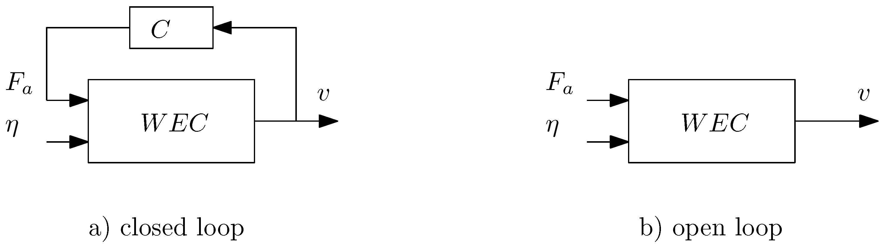
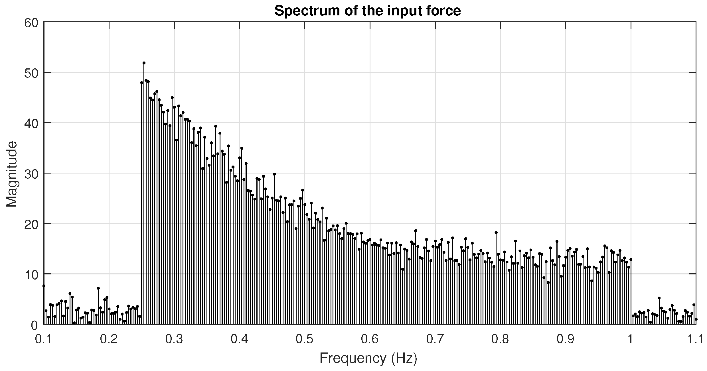
2.2. Experiments for System Identification
- Improved signal-to-noise ratio—For the same frequency resolution and RMS value, the signal-to-noise ratio is smaller; or for the same signal-to-noise ratio and RMS value, the measurement time is half as long.
- Increased range of physical regimes—Experiments where the system is tested using one input at the time (dual SISO) do not mimic the operational conditions, which may be a problem if the system behaves nonlinearly (i.e., single input tests may not reach the relevant physical regimes, therefore the test fails to observe important system dynamics).
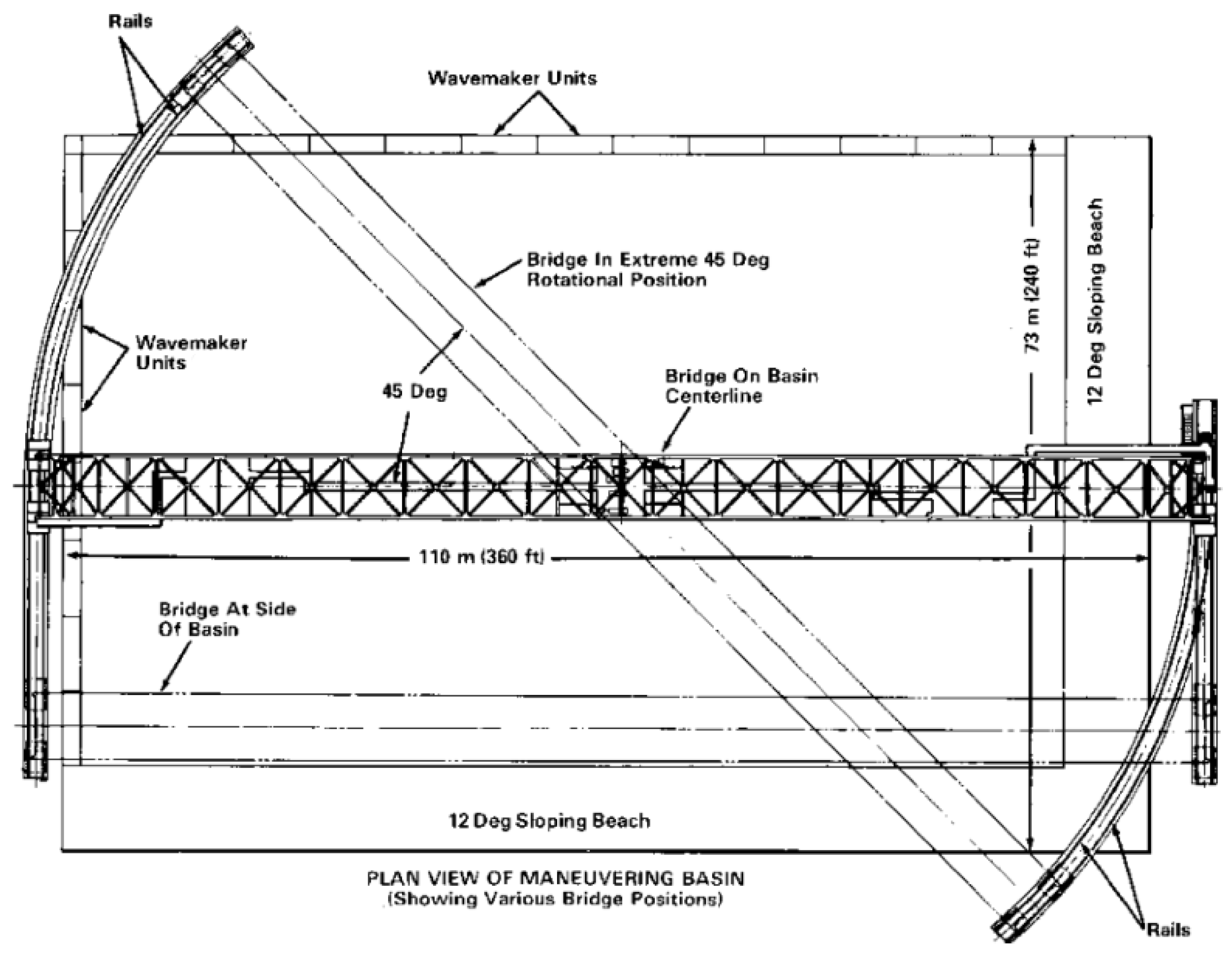
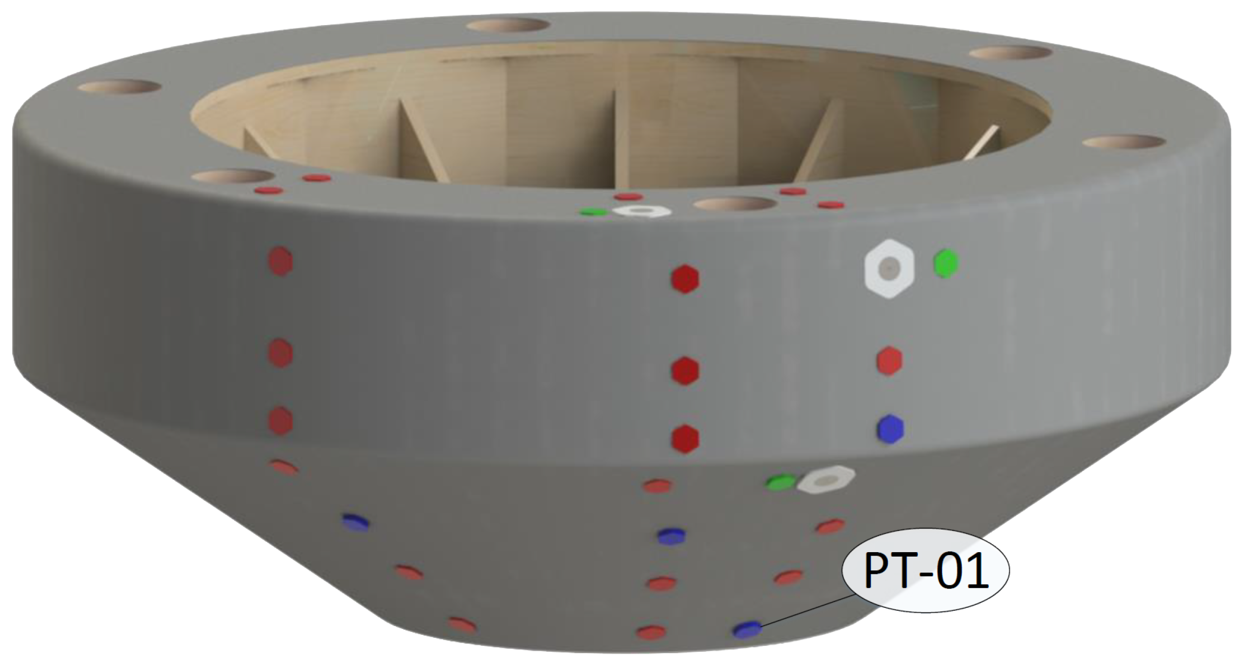
3. Description of Experimental Setup
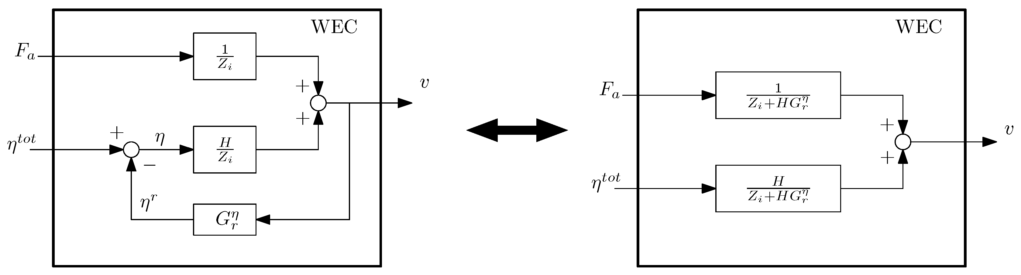
4. WEC Modeling in the Classical Framework: Radiation and Excitation
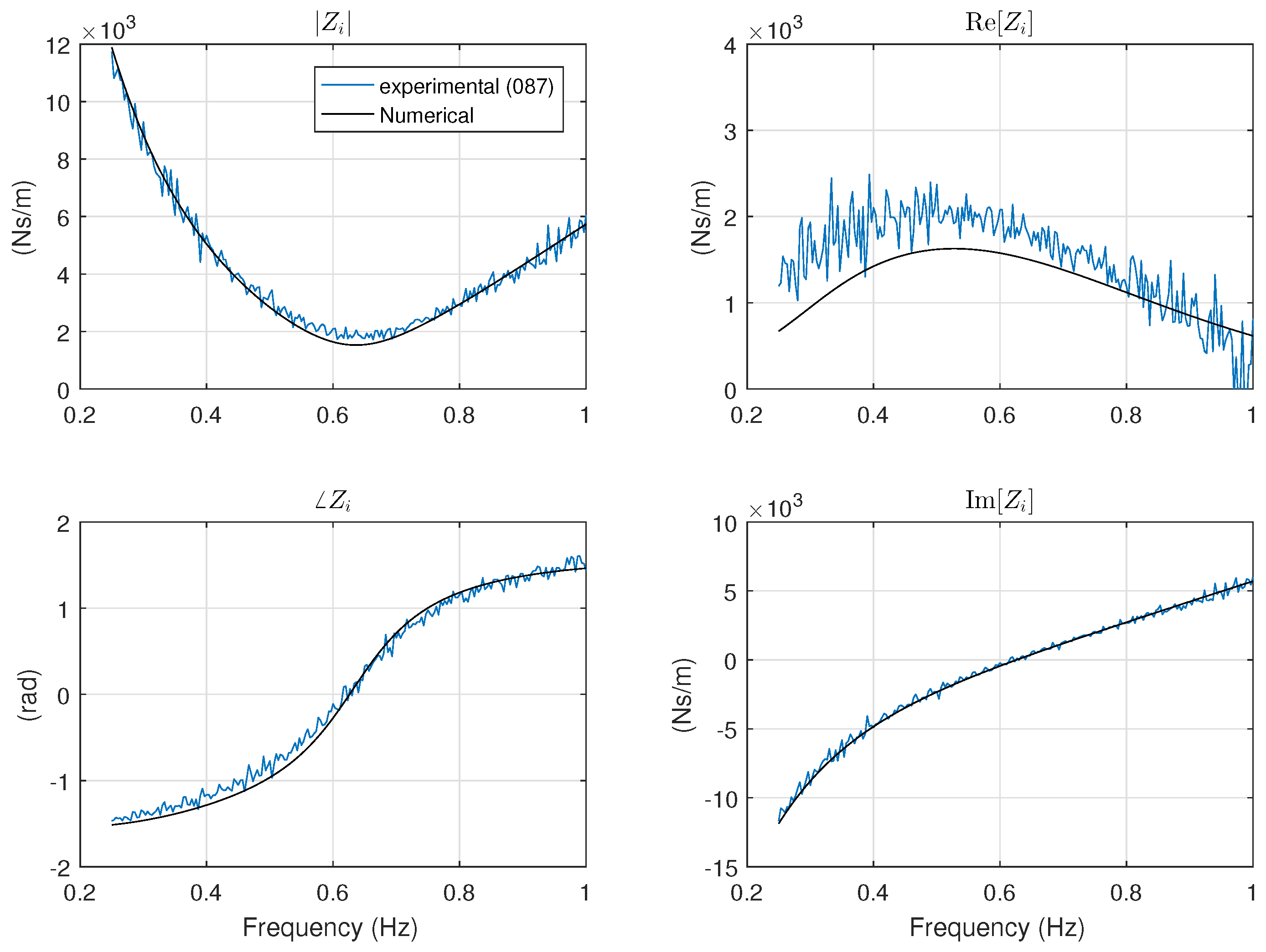
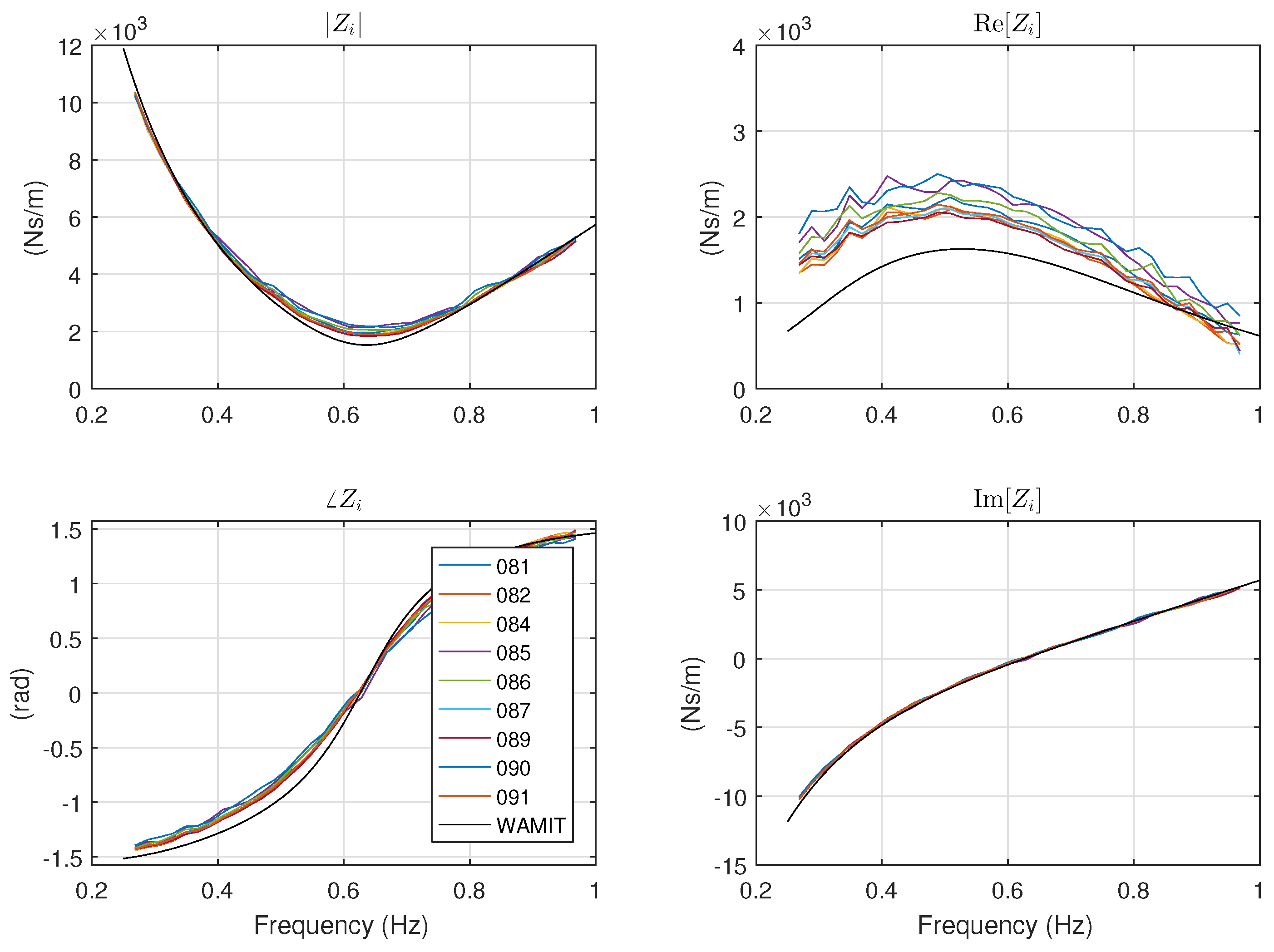
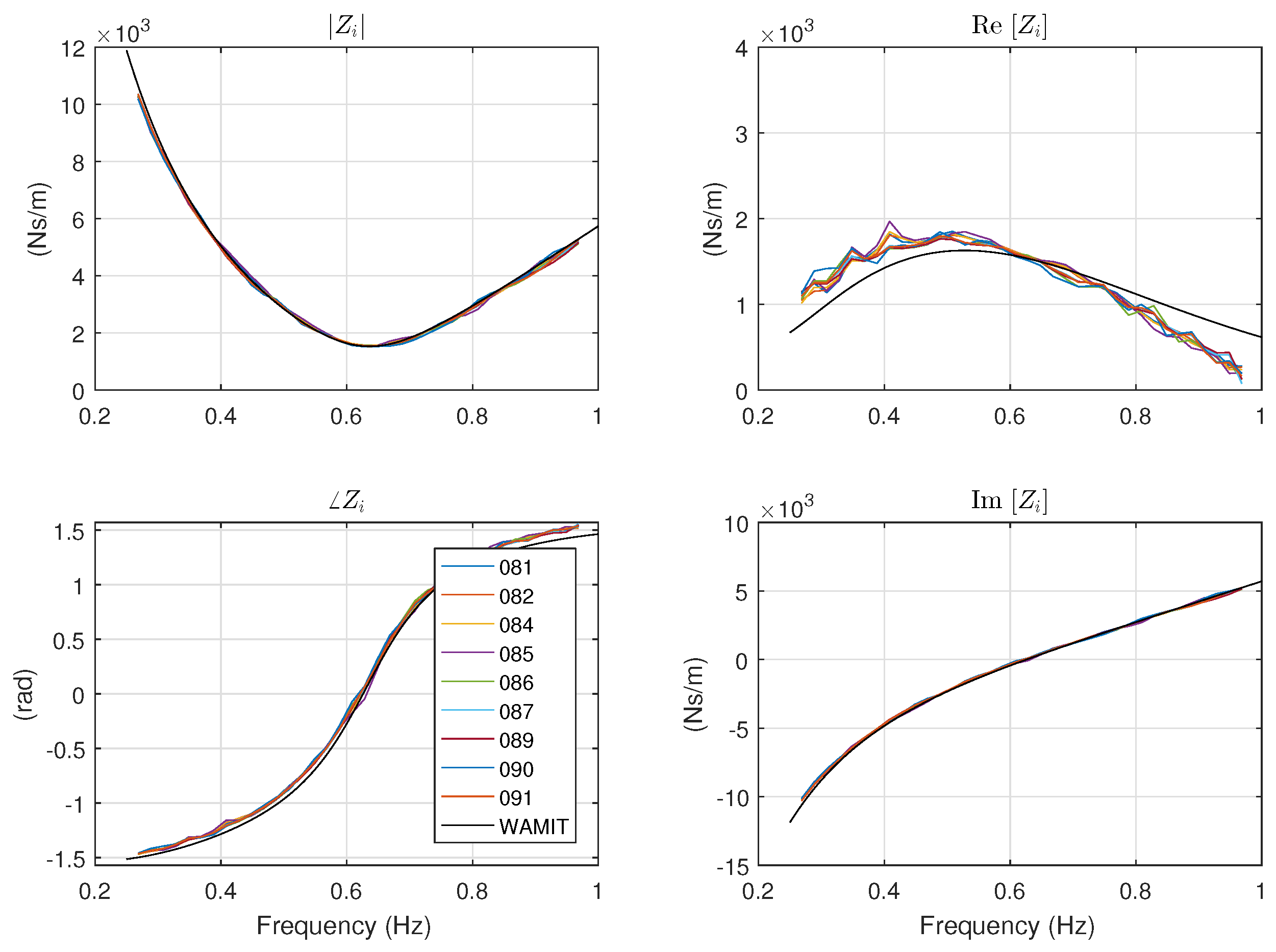
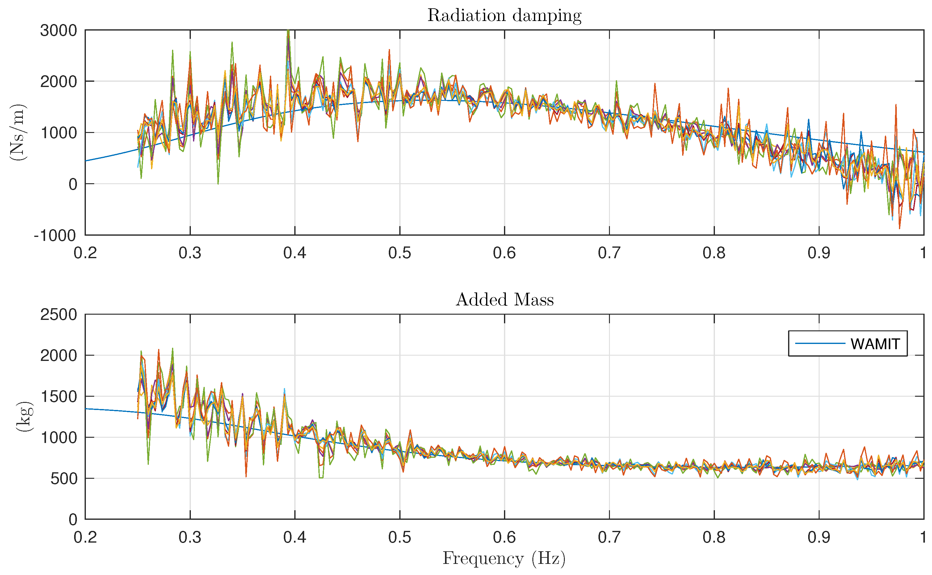
4.1. Intrinsic Impedance and Radiation Impedance
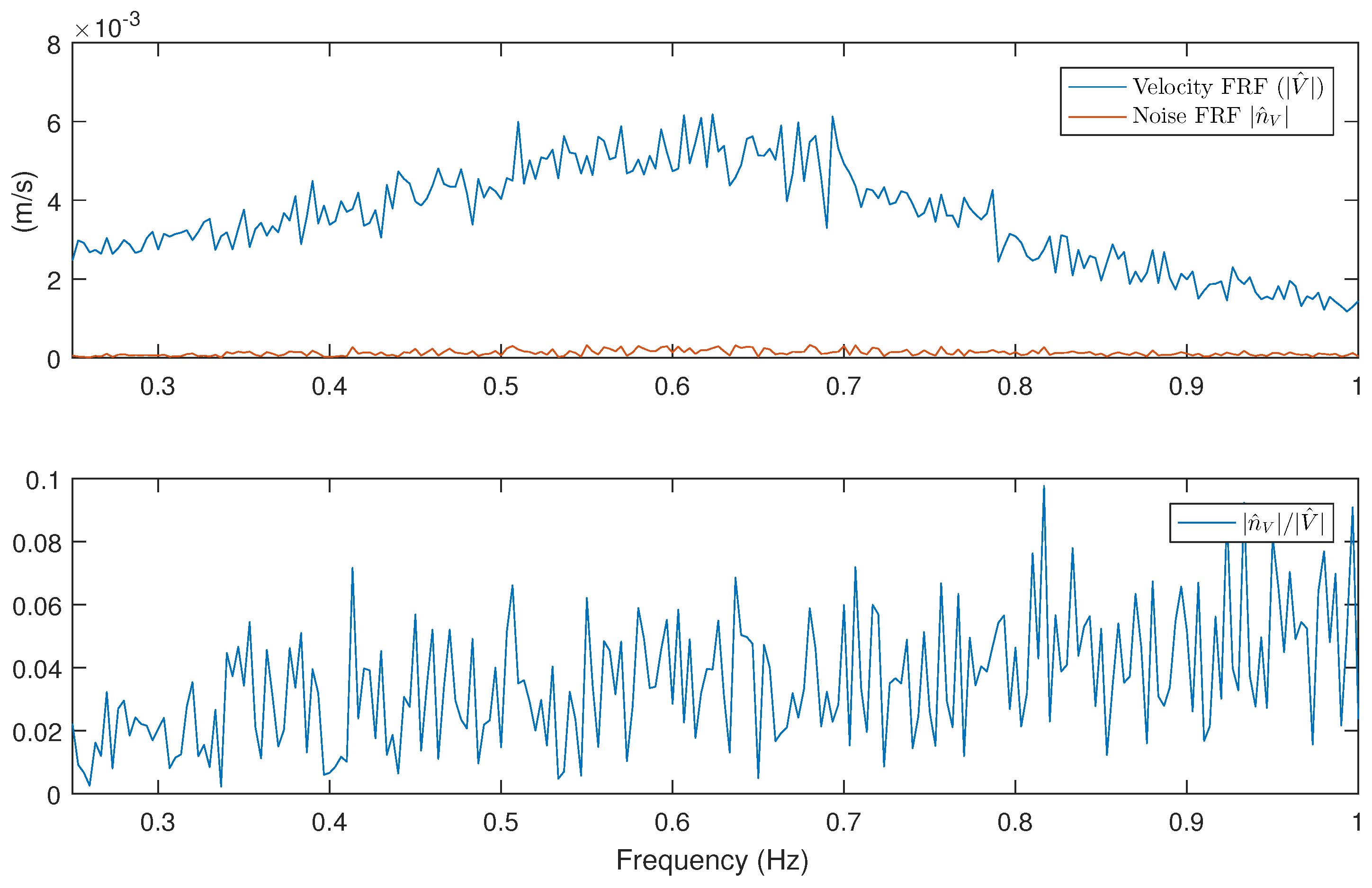
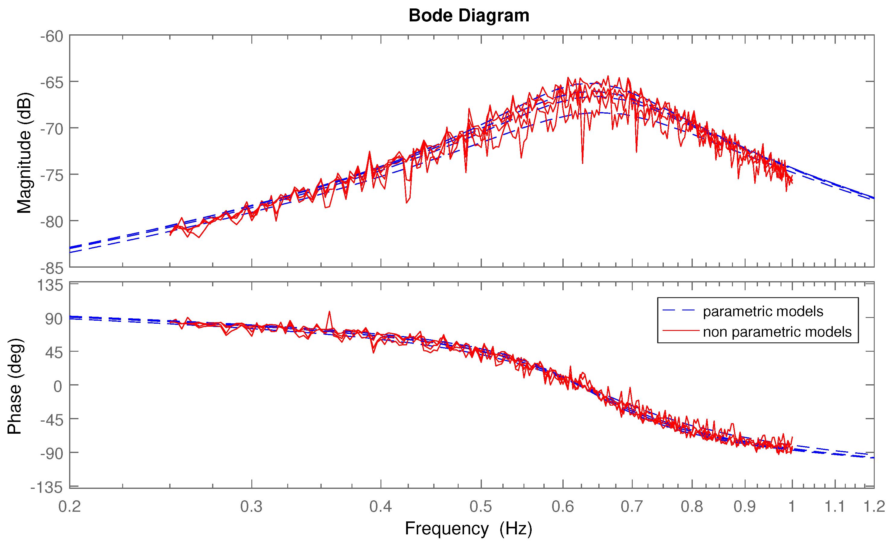
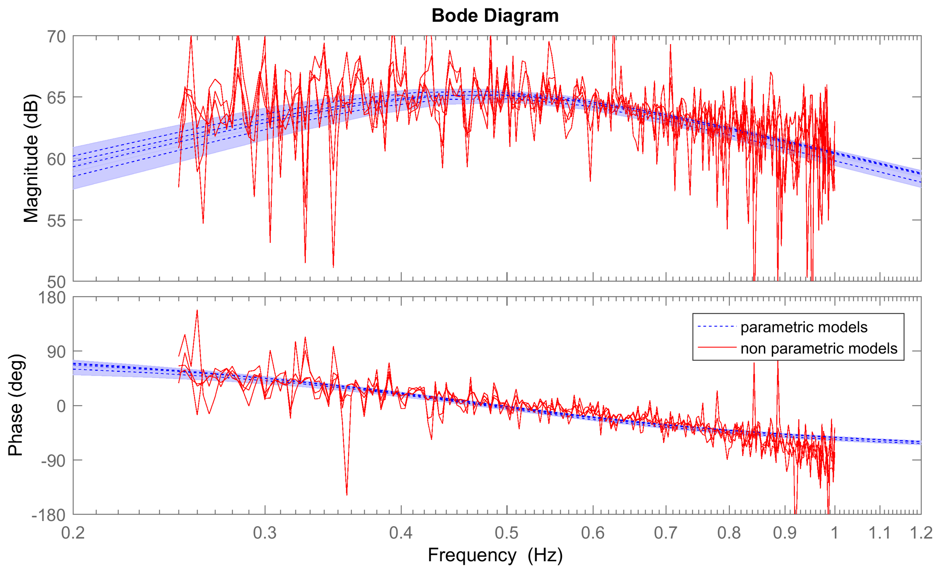
4.1.1. Nonparametric Models
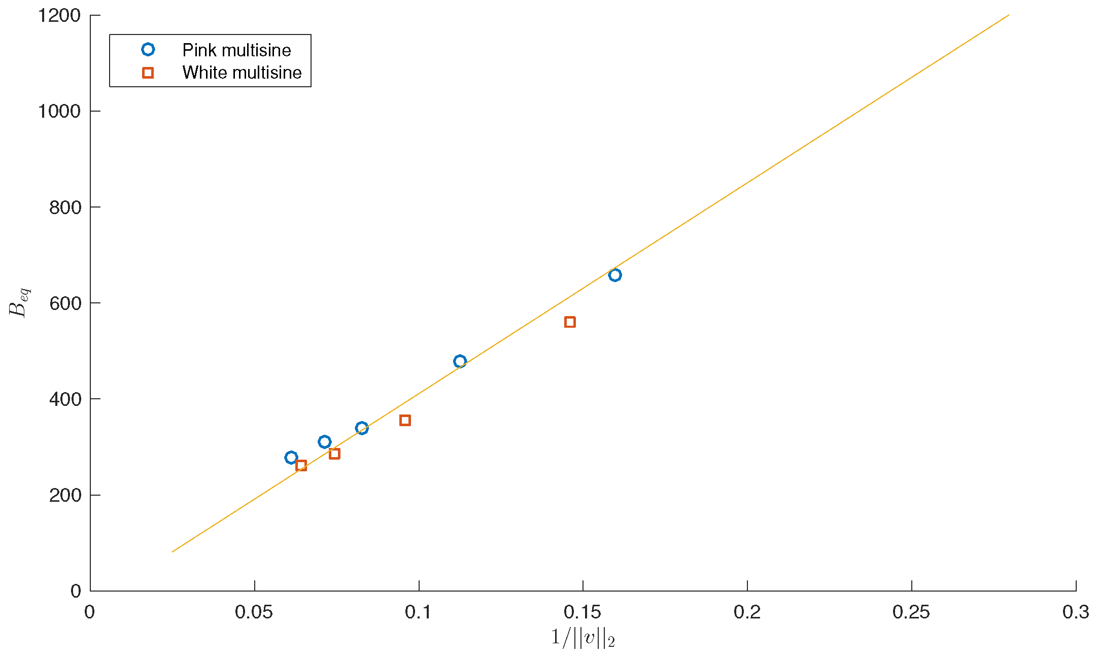
Radiation Force Modeling
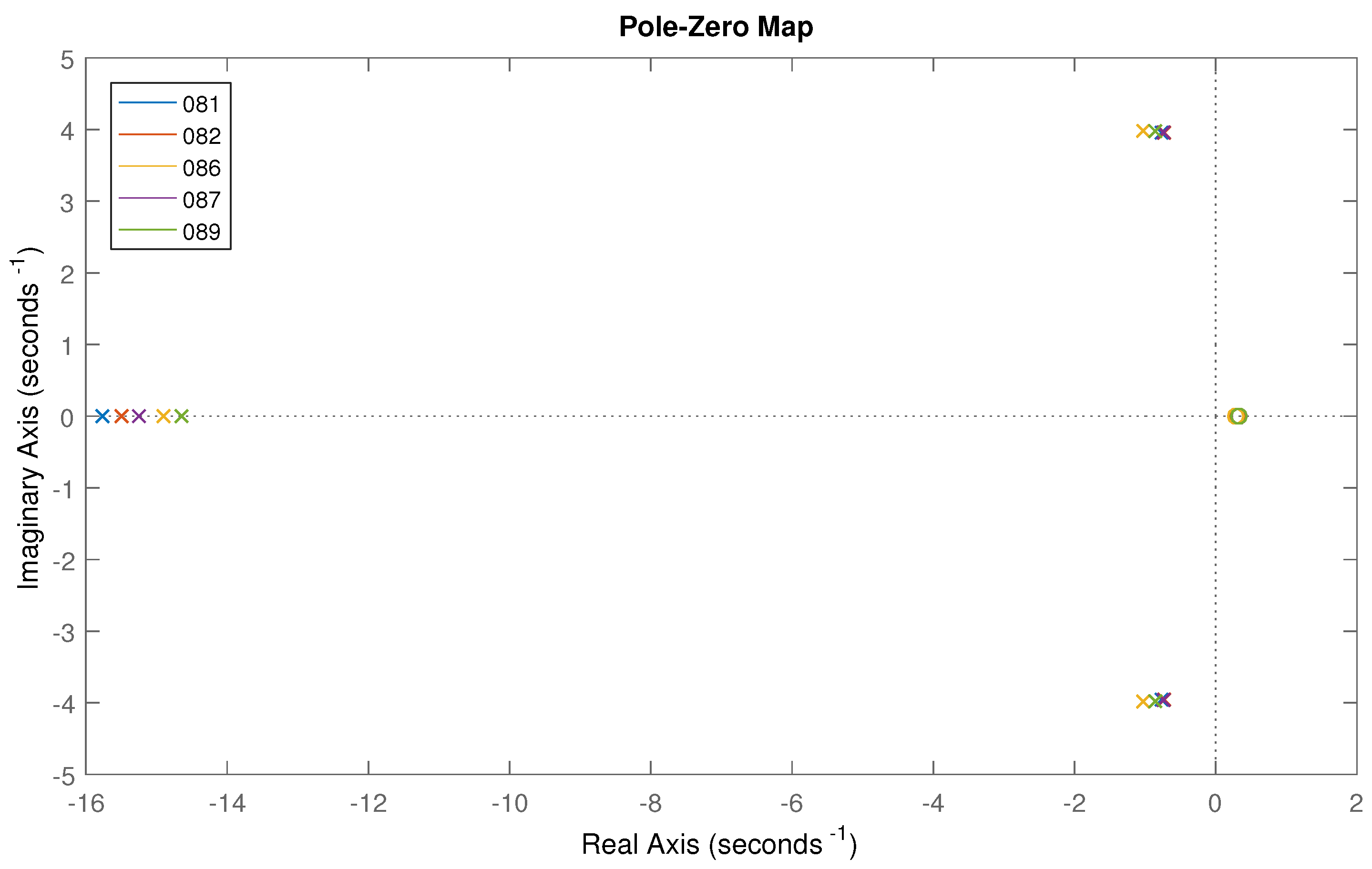
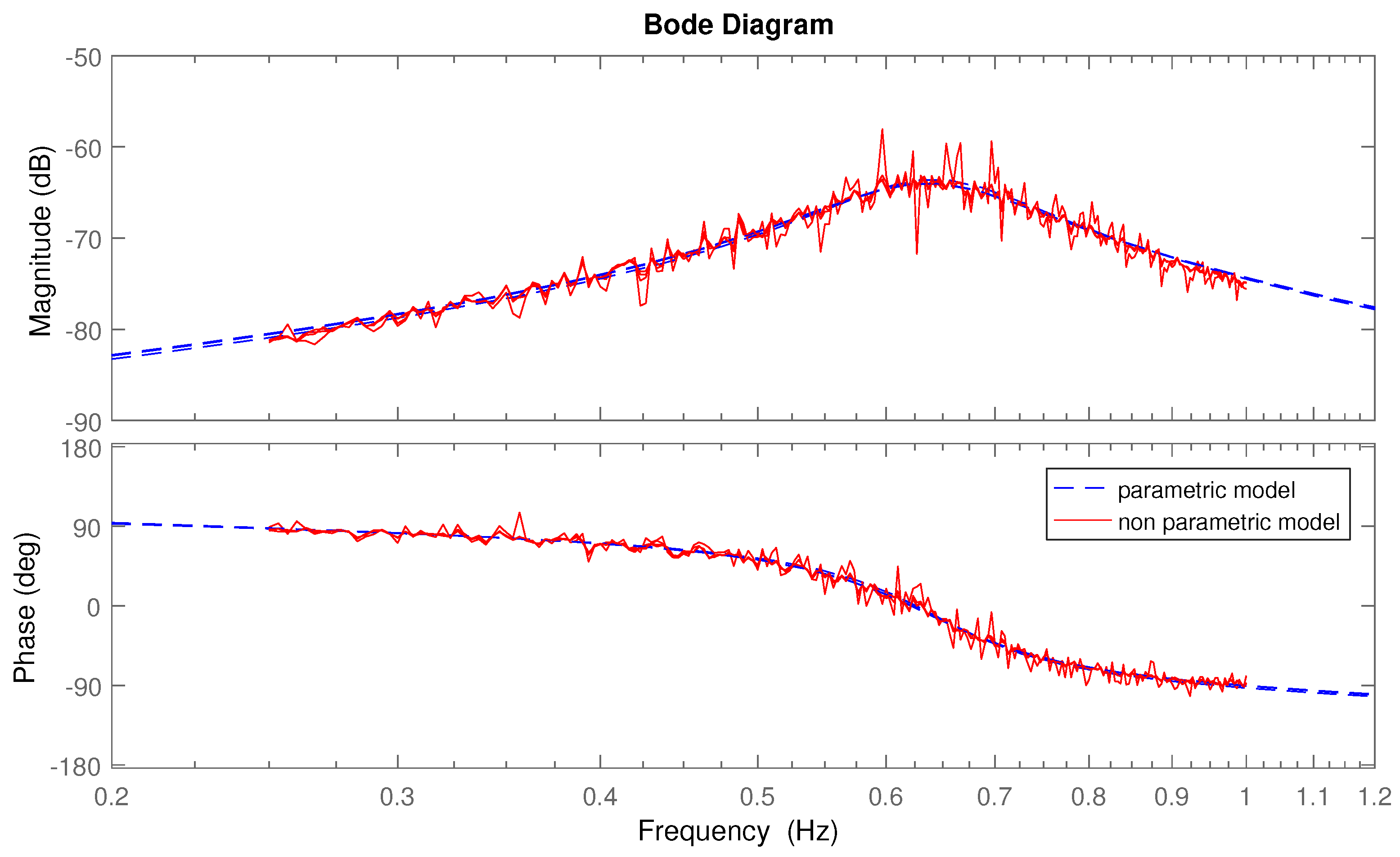
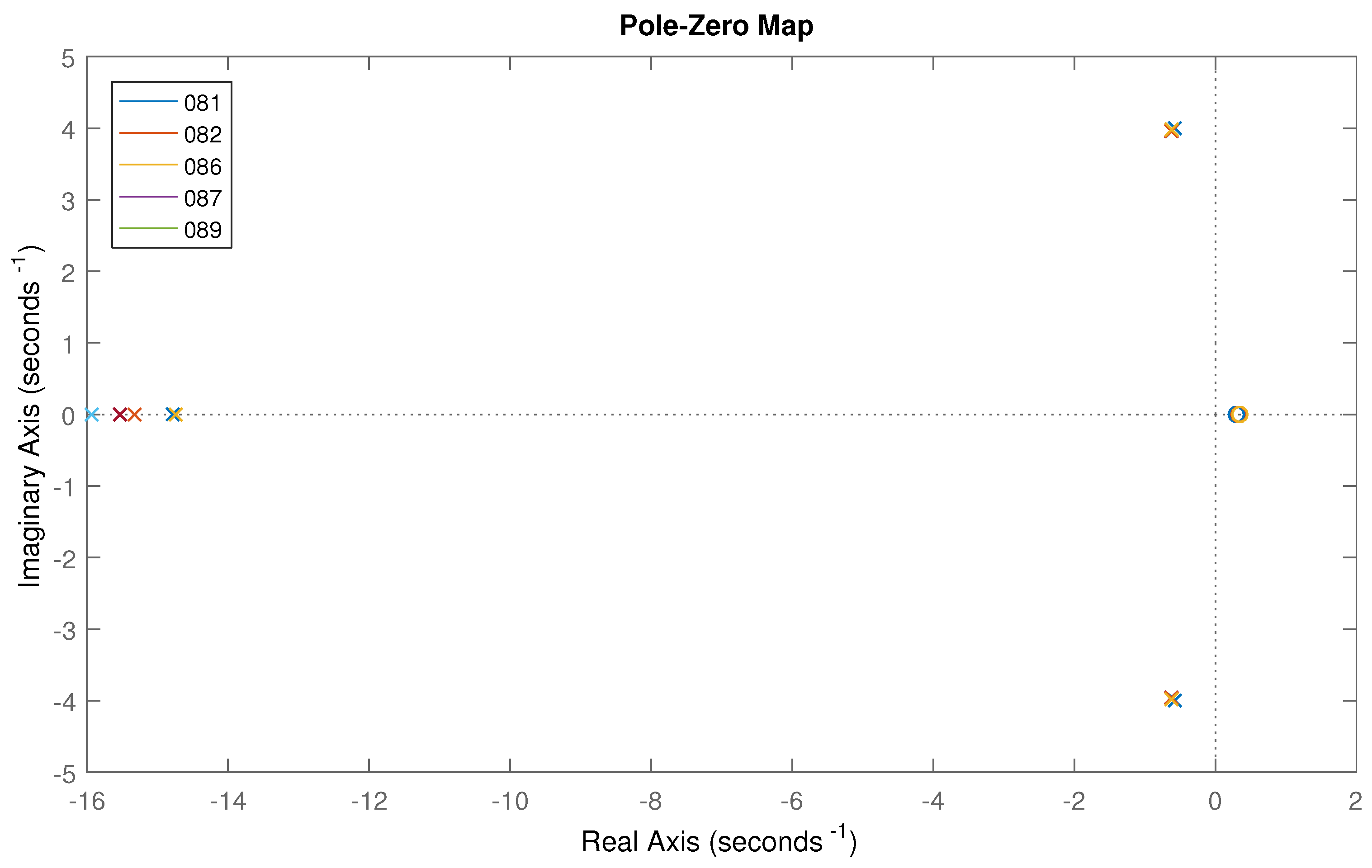
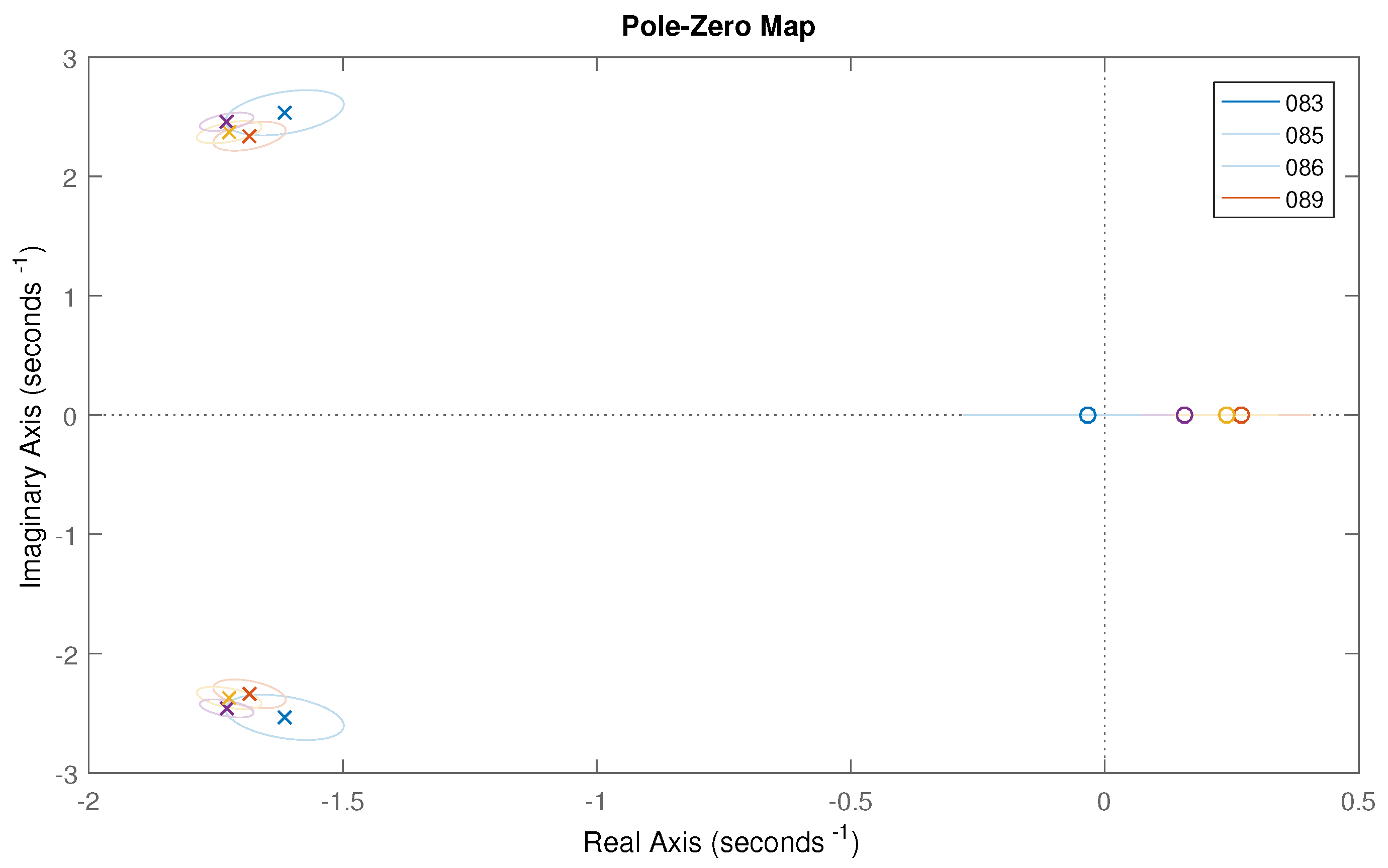
4.1.2. Parametric Models
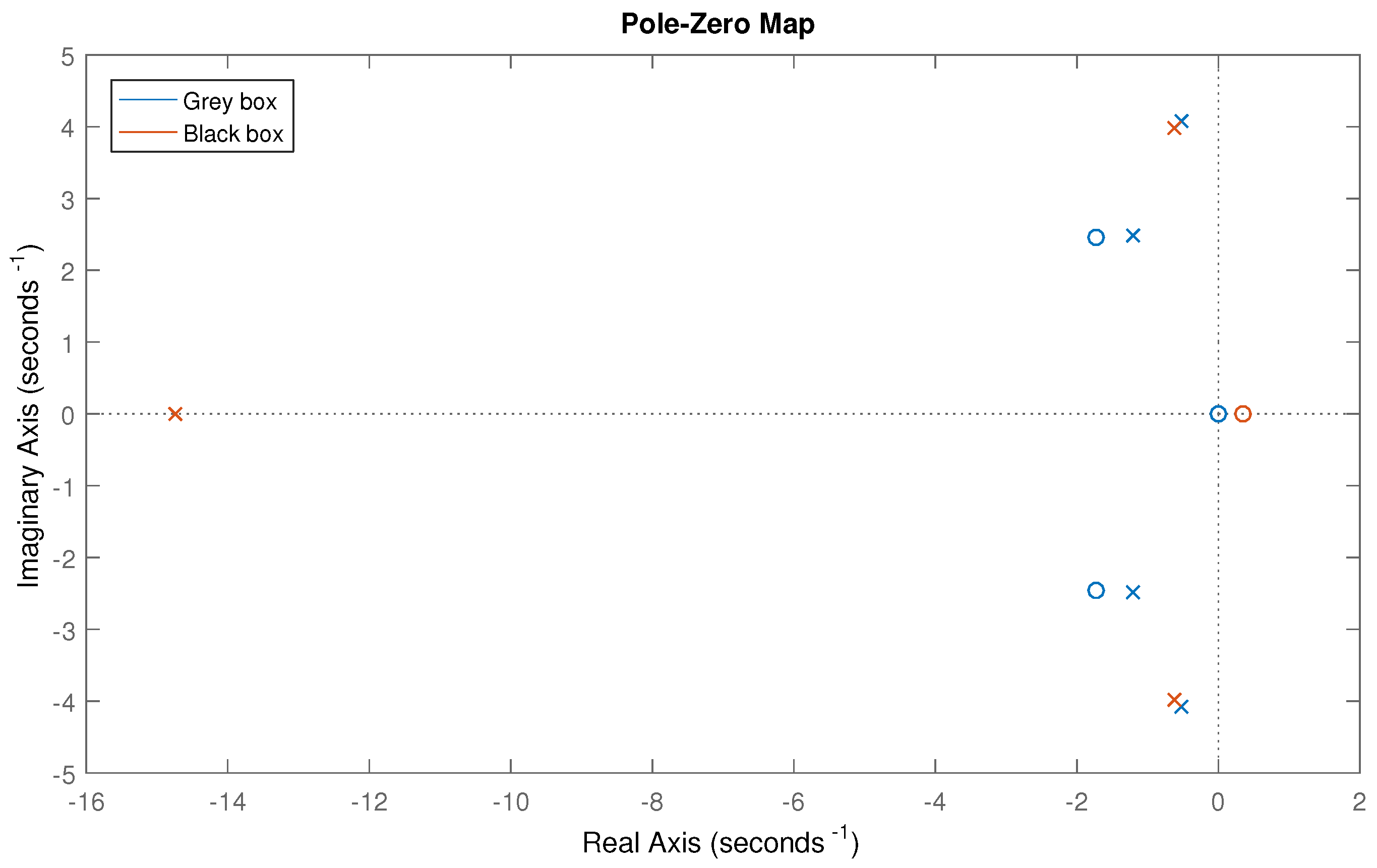
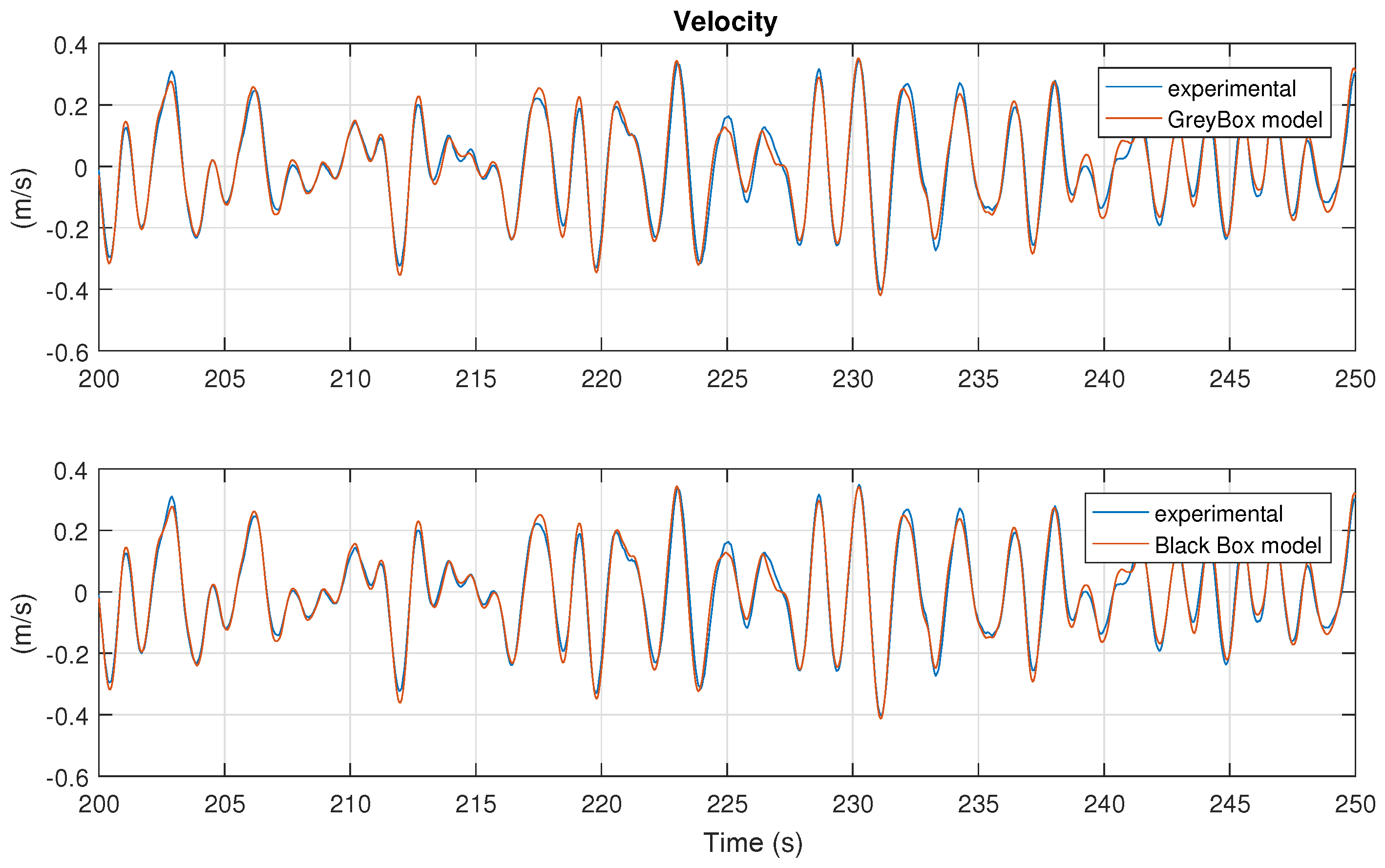
Black Box Modeling
Grey Box Modeling
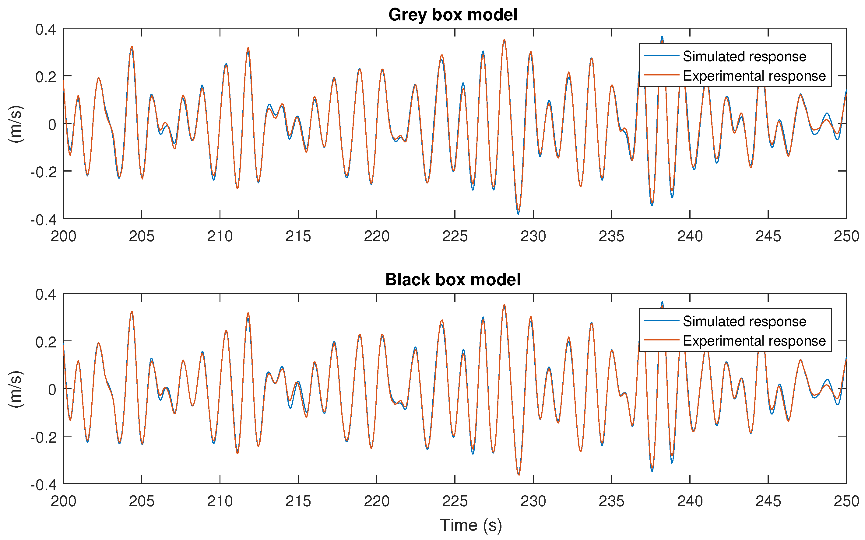
Comparison of Grey Box and Black Box Models, and Cross-Validation
4.2. Excitation Force Modeling
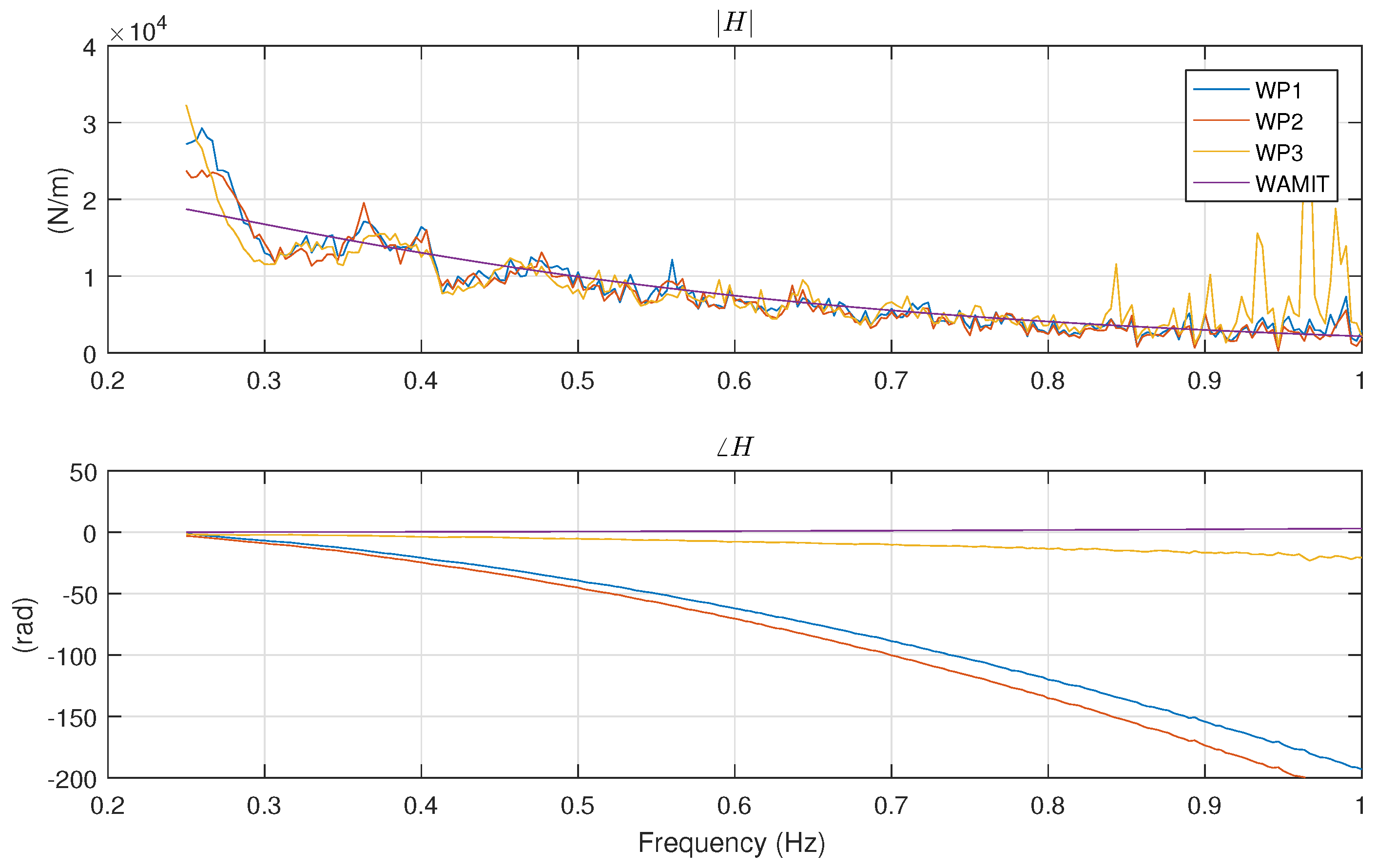
4.2.1. Estimation of the Excitation FRF from Diffraction Tests
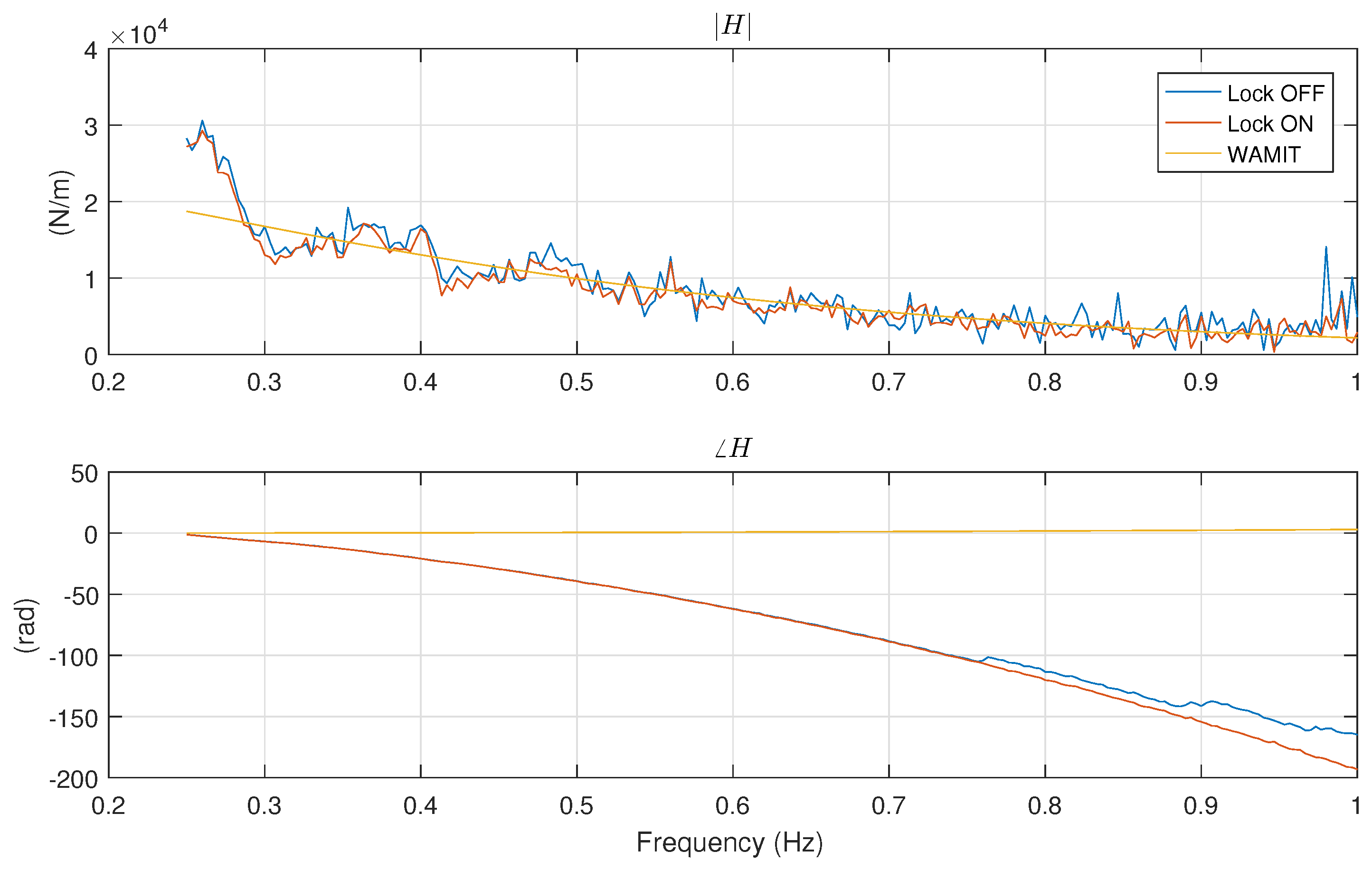
4.2.2. Estimation of the Excitation FRF without Locking the Buoy
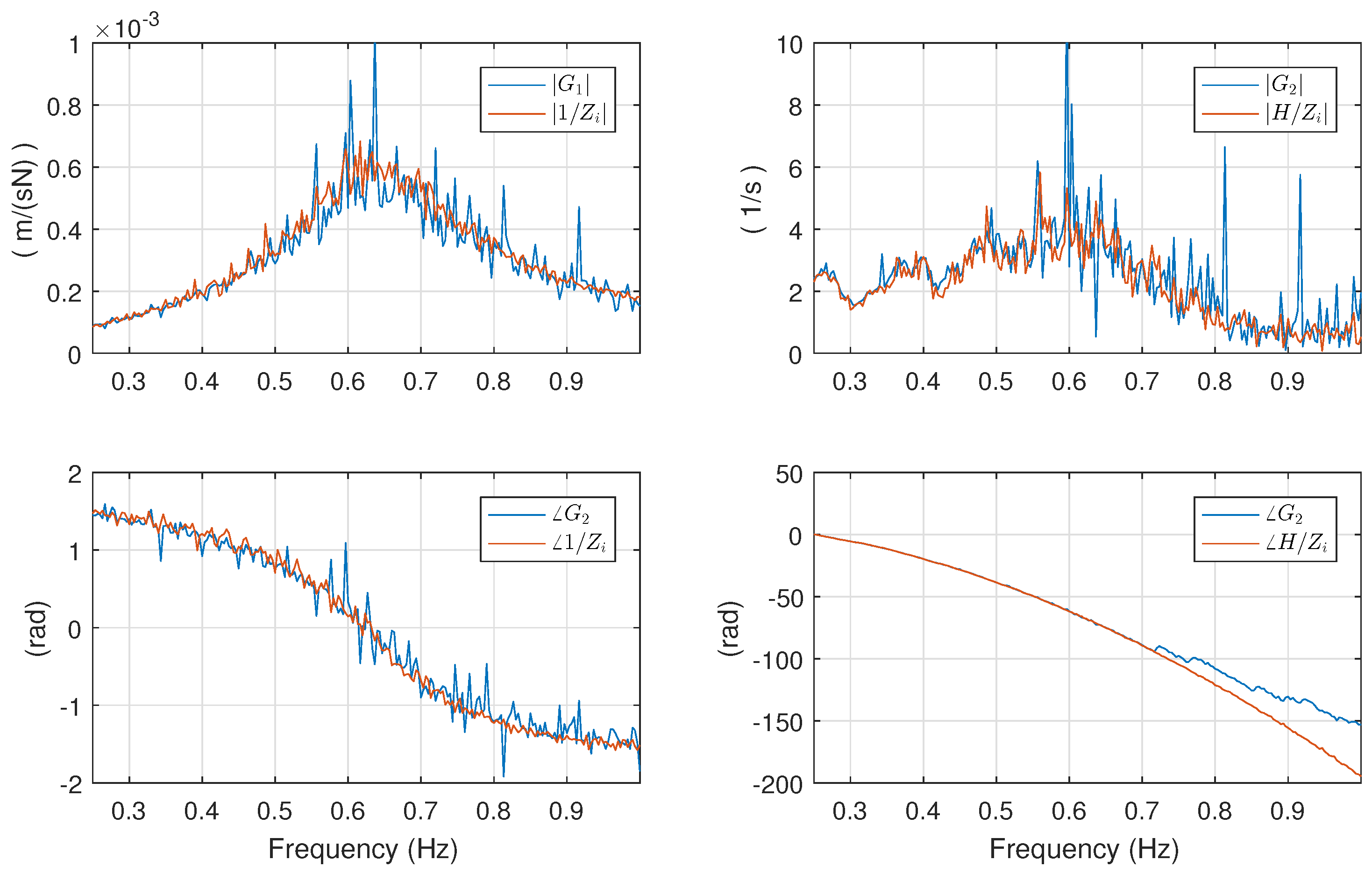
- Execute forced oscillation experiments in calm water to obtain a model of the intrinsic impedance as described in Section 4.1.1 and obtain either a parametric or nonparametric model for .
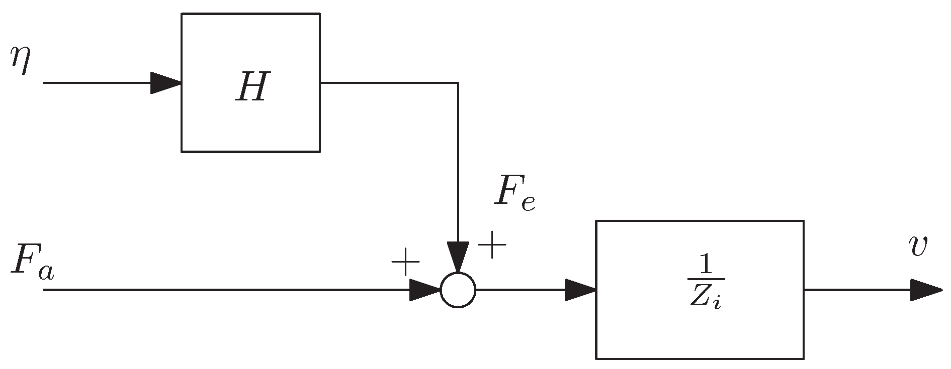
- Execute the forced oscillation experiment in presence of waves. In this case, the available measurements are the actuator force (), the buoy velocity (v) and the surface elevation (). By using the frequency-domain equation of motionit is possible to write the excitation FRF as function of the known quantities as:
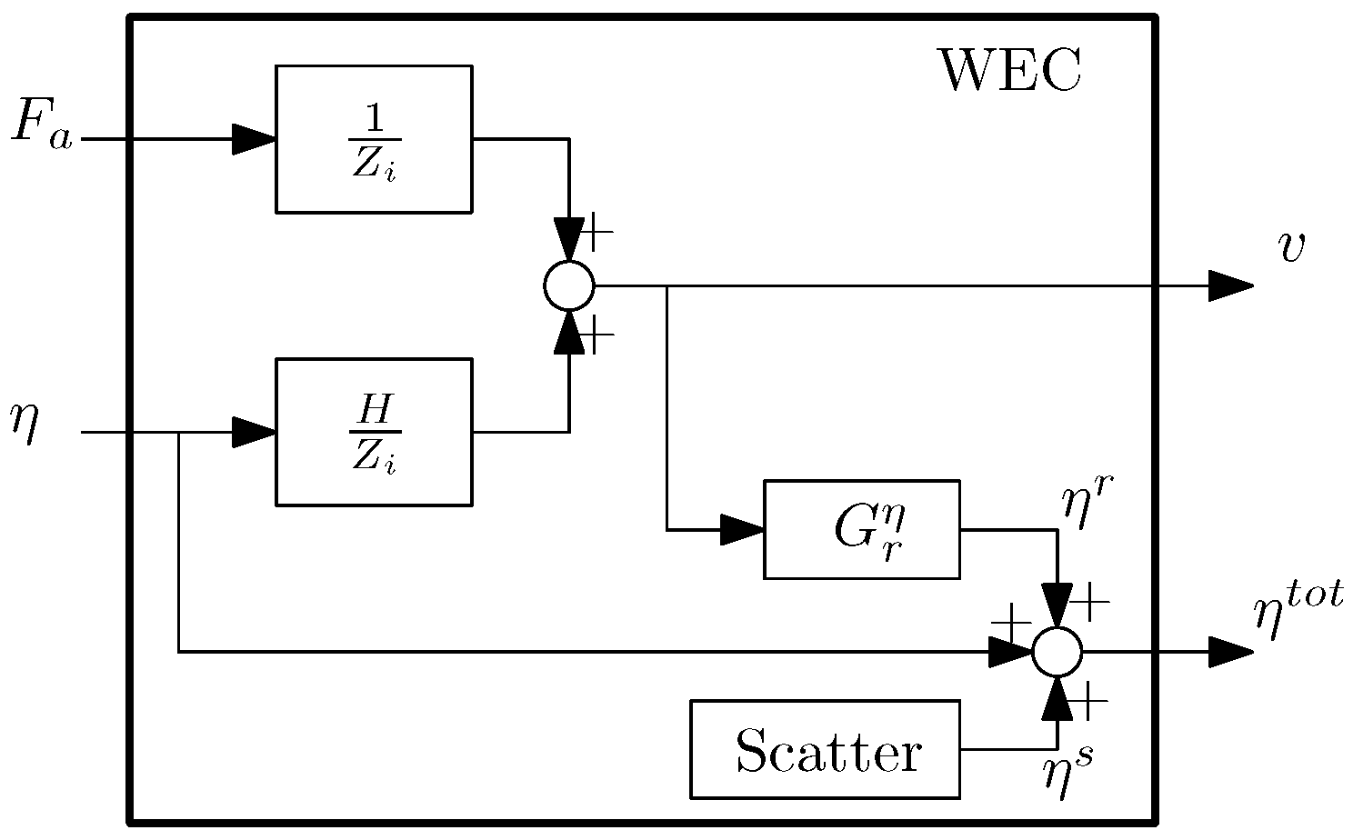
4.3. Validation of Combined Model
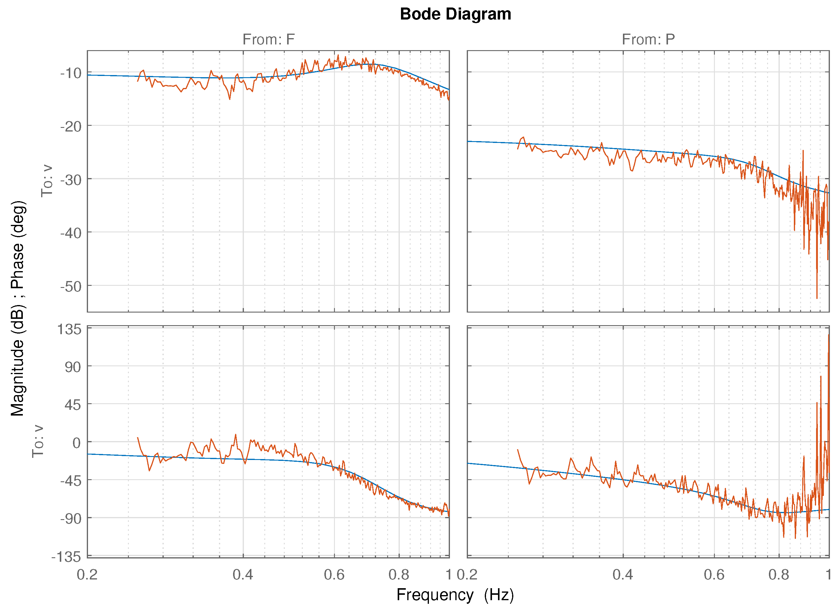
4.4. WEC Model as Multiple-Input Single-Output System
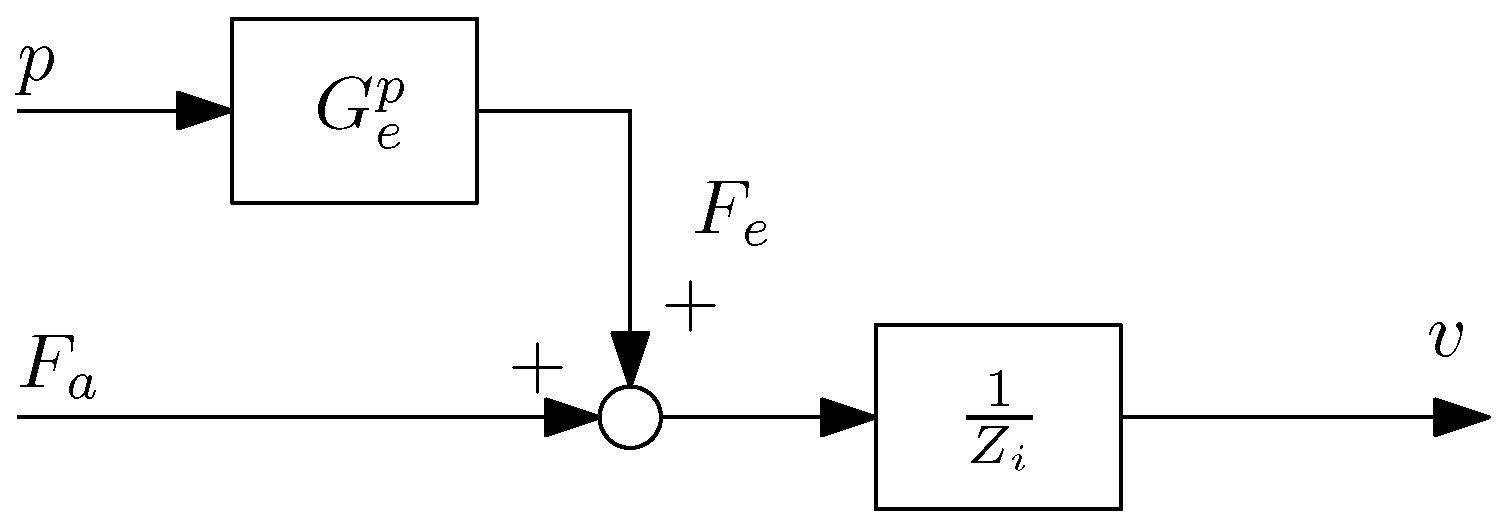
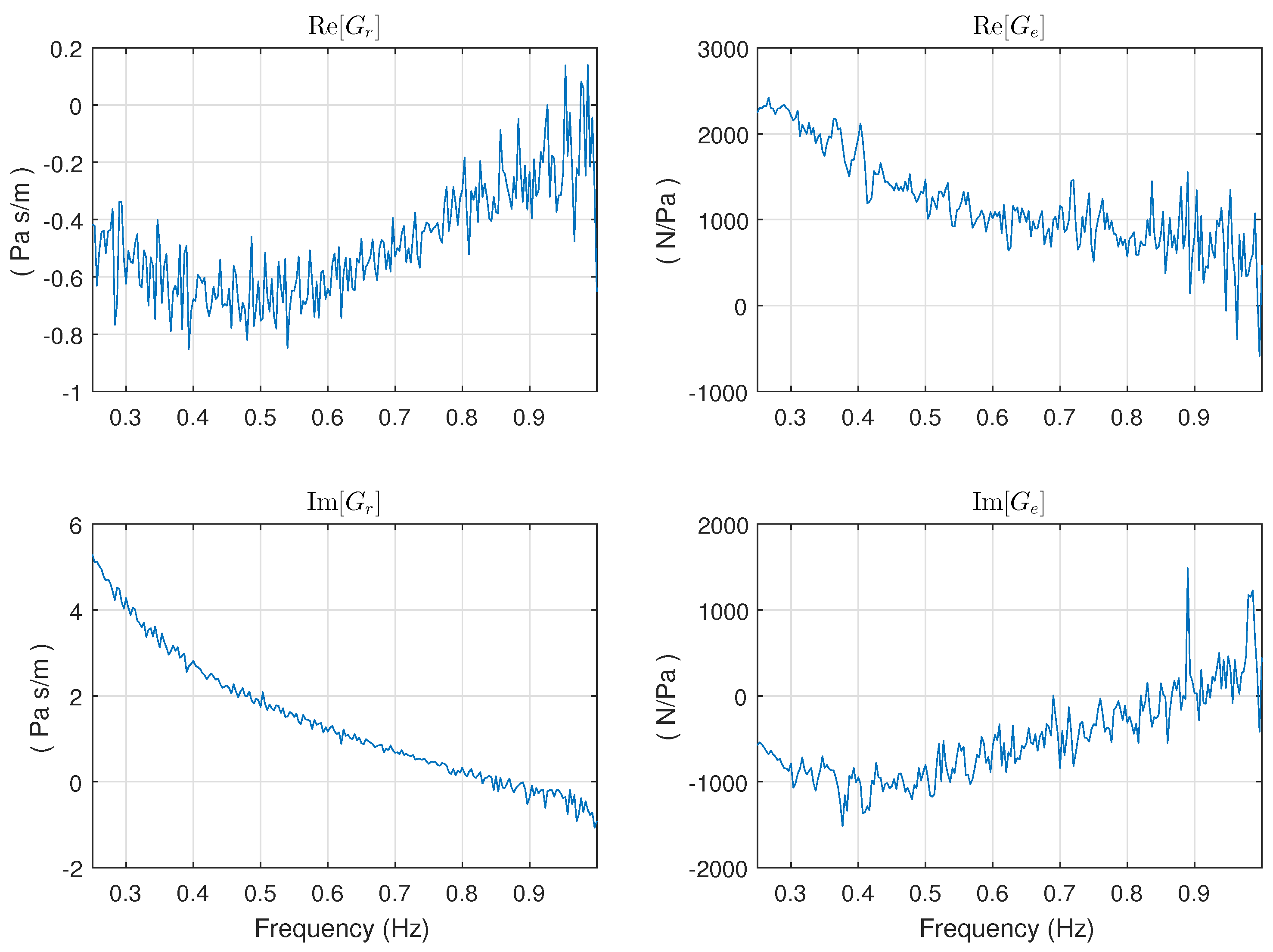
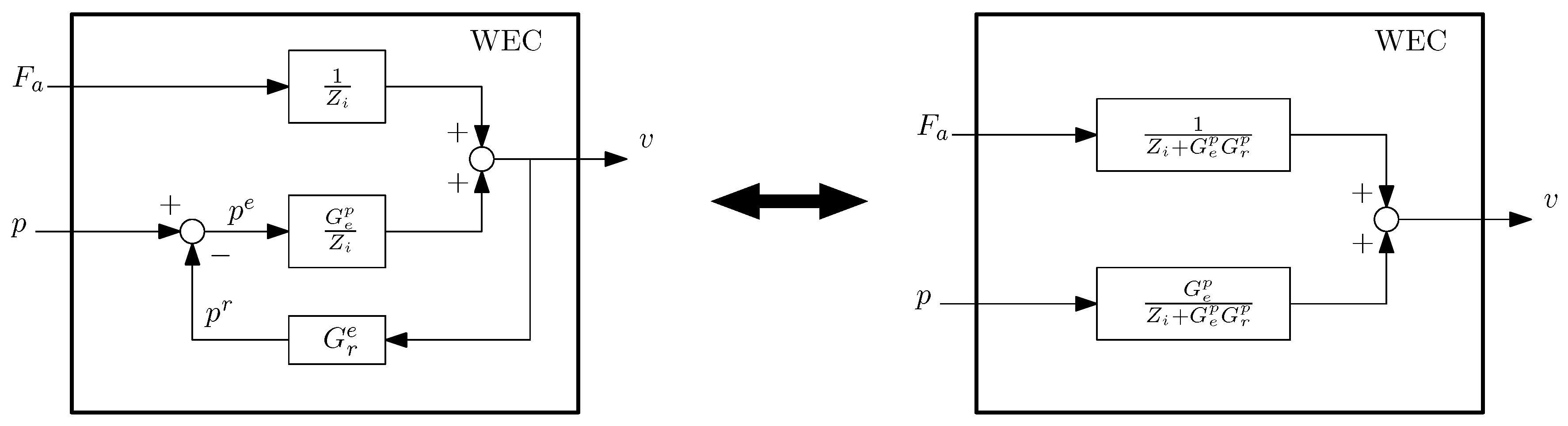
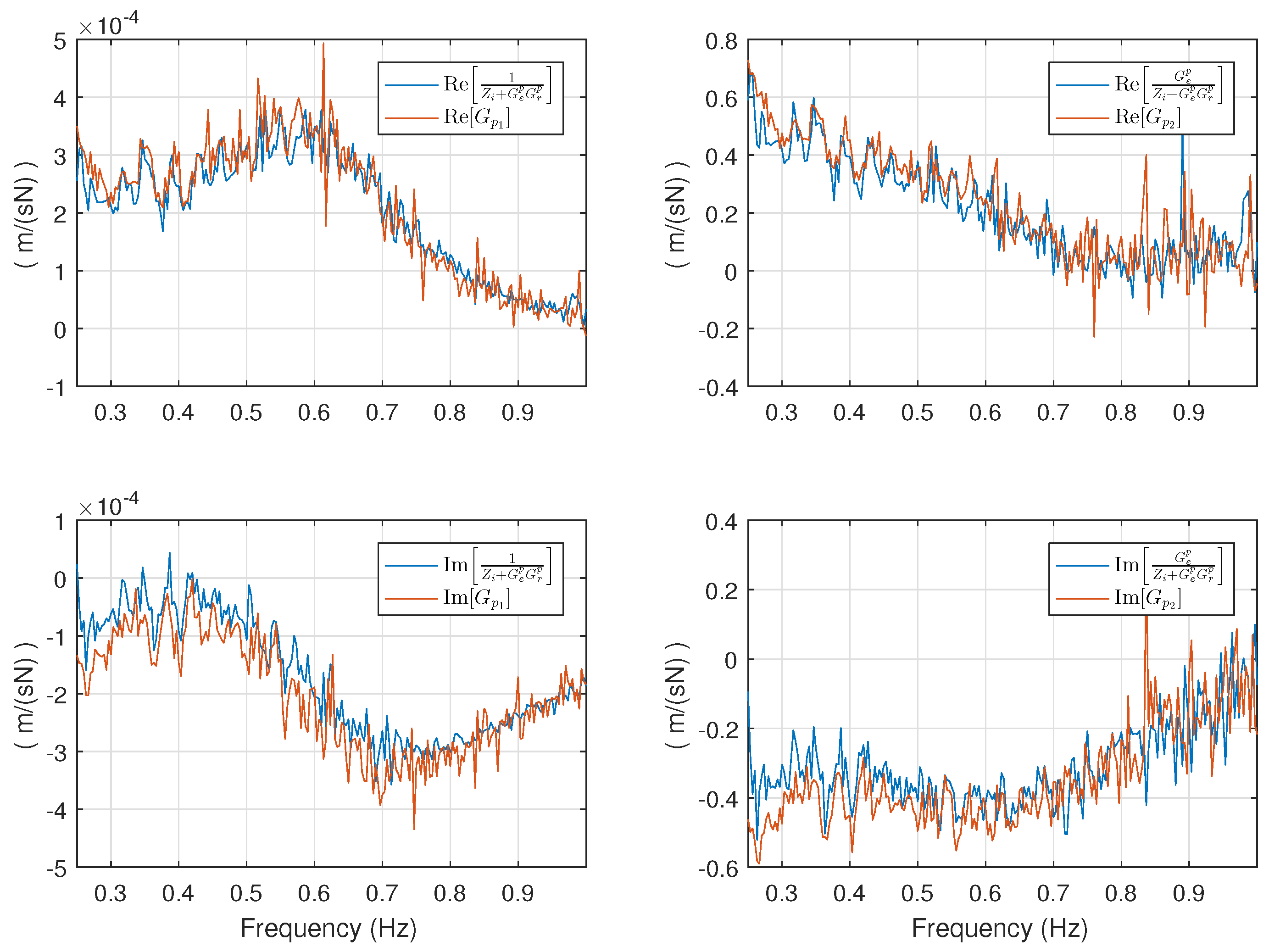
5. WEC Modeling Using Pressure
6. Discussion and Conclusions
Acknowledgments
Author Contributions
Conflicts of Interest
Abbreviations
| BEM | Boundary element method |
| FRF | Frequency response function |
| FRM | Frequency response matrix |
| FFT | Fast Fourier transform |
| LTI | Linear time invariant |
| IRF | Impulse response function |
| MASK | Maneuvering And Sea Keeping |
| MISO | Multiple input single-output |
| NRMSE | Normalized root mean square error |
| PTO | Power take-off |
| SID | System identification |
| SISO | Single input single output |
| WEC | Wave energy converter |
References
- Hals, J.; Falnes, J.; Moan, T. A Comparison of Selected Strategies for Adaptive Control of Wave Energy Converters. J. Offshore Mech. Arct. Eng. 2011, 133, 031101. [Google Scholar] [CrossRef]
- Wilson, D.; Bacelli, G.; Coe, R.G.; Bull, D.L.; Abdelkhalik, O.; Korde, U.A.; Robinett III, R.D. A Comparison of WEC Control Strategies; Technical Report SAND2016-4293; Sandia National Labs: Albuquerque, NM, USA, 2016. [Google Scholar]
- WAMIT. WAMIT User Manual, 7th ed.; Wave Analysis MIT (WAMIT): Chestnut Hill, MA, USA, 2012. [Google Scholar]
- Babarit, A.; Delhommeau, G. Theoretical and numerical aspects of the open source BEM solver NEMOH. In Proceedings of the 11th European Wave and Tidal Energy Conference (EWTEC2015), Nantes, France, 6–11 September 2015. [Google Scholar]
- Ljung, L. System Identification—Theory for the User; Prentice-Hall PTR: Upper Saddle River, NJ, USA, 1999. [Google Scholar]
- Pintelon, R.; Schoukens, J. System Identification: A Frequency Domain Approach; John Wiley & Sons: Hoboken, NJ, USA, 2012. [Google Scholar]
- Giorgi, S.; Davidson, J.; Ringwood, J.V. Identification of Wave Energy Device Models From Numerical Wave Tank Data Part 2: Data-Based Model Determination. IEEE Trans. Sustain. Energy 2016, 7, 1020–1027. [Google Scholar] [CrossRef]
- Davidson, J.; Giorgi, S.; Ringwood, J.V. Linear parametric hydrodynamic models for ocean wave energy converters identified from numerical wave tank experiments. Ocean Eng. 2015, 103, 31–39. [Google Scholar] [CrossRef]
- Cummins, W.E. The Impulse Response Function and Ship Motions; Technical Report DTNSDRC 1661; Department of the Navy, David Taylor Model Basin: Bethesda, MD, USA, 1962. [Google Scholar]
- Falnes, J. Ocean Waves and Oscillating Systems; Cambridge University Press: Cambridge, UK; New York, NY, USA, 2002. [Google Scholar]
- Yu, Z.; Falnes, J. State-space modelling of a vertical cylinder in heave. Appl. Ocean Res. 1995, 17, 265–275. [Google Scholar] [CrossRef]
- Perez, T.; Fossen, T.I. Time- vs. Frequency-domain Identification of Parametric Radiation Force Models for Marine Structures at Zero Speed. Model. Identif. Control 2008, 29, 1–19. [Google Scholar] [CrossRef]
- Billings, S.A.; Lang, Z.Q. Truncation of nonlinear system expansions in the frequency domain. Int. J. Control 1997, 68, 1019–1042. [Google Scholar] [CrossRef]
- Schoukens, J.; Vaes, M.; Pintelon, R. Linear System Identification in a Nonlinear Setting: Nonparametric Analysis of the Nonlinear Distortions and Their Impact on the Best Linear Approximation. IEEE Control Syst. 2016, 36, 38–69. [Google Scholar] [CrossRef]
- Coe, R.G.; Bacelli, G.; Patterson, D.; Wilson, D.G. Advanced WEC Dynamics & Controls FY16 Testing Report; Technical Report SAND2016-10094; Sandia National Labs: Albuquerque, NM, USA, 2016.
- Brownell, W. Two New Hydromechanics Research Facilities at the David Taylor Model Basin; Technical Report 1690; Department Of The Navy, David Taylor Model Basin: Bethesda, MD, USA, 1962. [Google Scholar]
- Advanced WEC Dynamics and Controls, Test 1—Experimental Data Hosted on the “Marine and Hydrokinetic Data Repository”. U.S. DEPARTMENT OF ENERGY. Available online: https://mhkdr.openei.org/submissions/151 (accessed on 30 December 2016).
- Perez, T.; Fossen, T.I. A Matlab Toolbox for Parametric Identification of Radiation-Force Models of Ships and Offshore Structures. Model. Identif. Control A Nor. Res. Bull. 2009, 30, 1–15. [Google Scholar] [CrossRef]
- Ogata, K. Modern Control Engineering; Prentice Hall: Upper Saddle River, NJ, USA, 2002. [Google Scholar]
- Duclos, G.; Clement, A.; Chatry, G. Absorption of Outgoing Waves in a numerical wave tank using a self-adaptive boundary condition. In Proceedings of the 10th Int Offshore and Polar Engineering Conference ISOPE 2000, Seattle, WA, USA, 27 May–2 June 2000. [Google Scholar]
- Falnes, J. On non-causal impulse response functions related to propagating water waves. Appl. Ocean Res. 1995, 17, 379–389. [Google Scholar] [CrossRef]


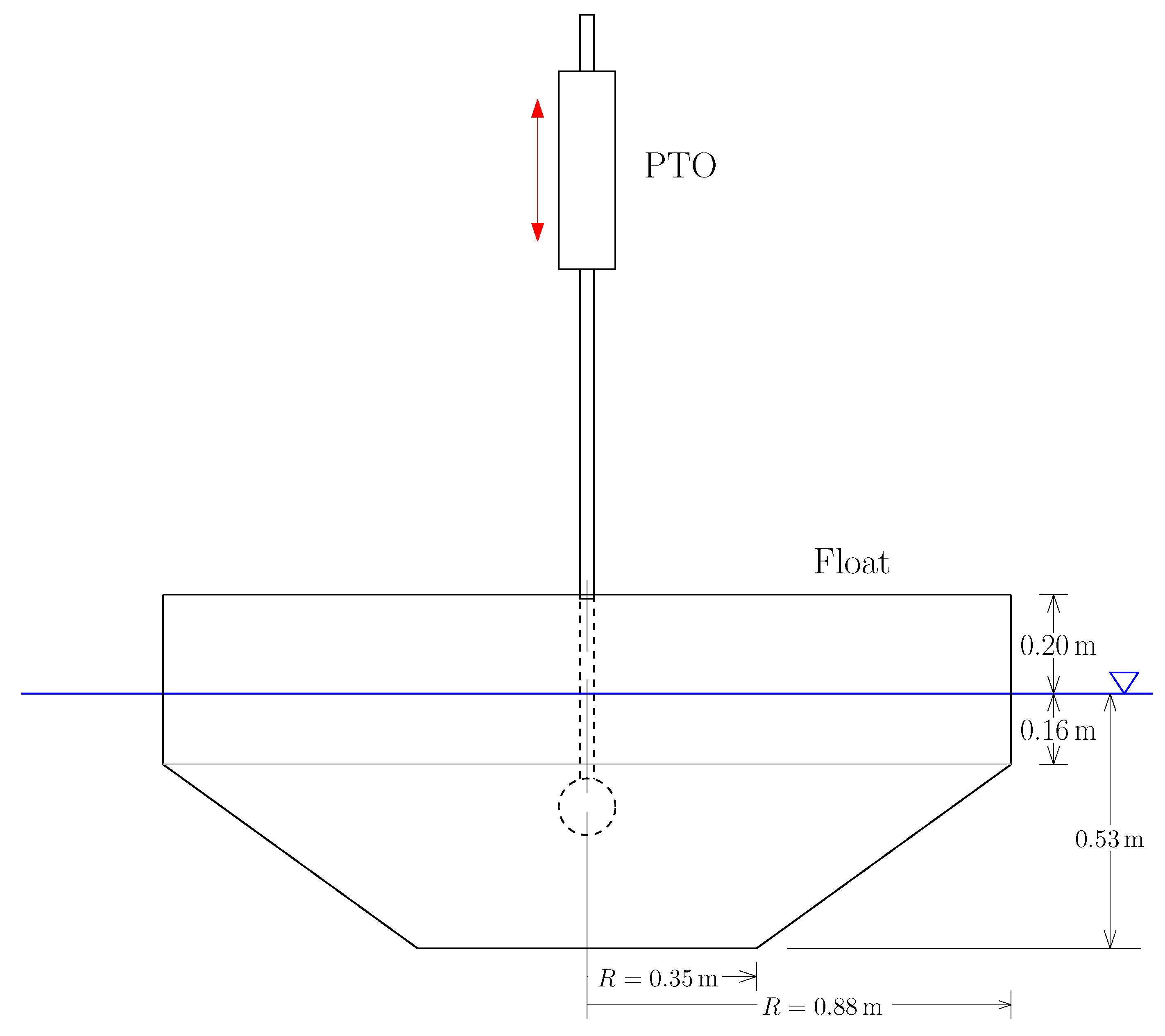
| Parameter | Value |
|---|---|
| Rigid-body mass (float & slider), M (kg) | 858 |
| Displaced volume, ∀ (m3) | 0.858 |
| Float radius, r (m) | 0.88 |
| Float draft, T (m) | 0.53 |
| Water density, (kg/m3) | 1000 |
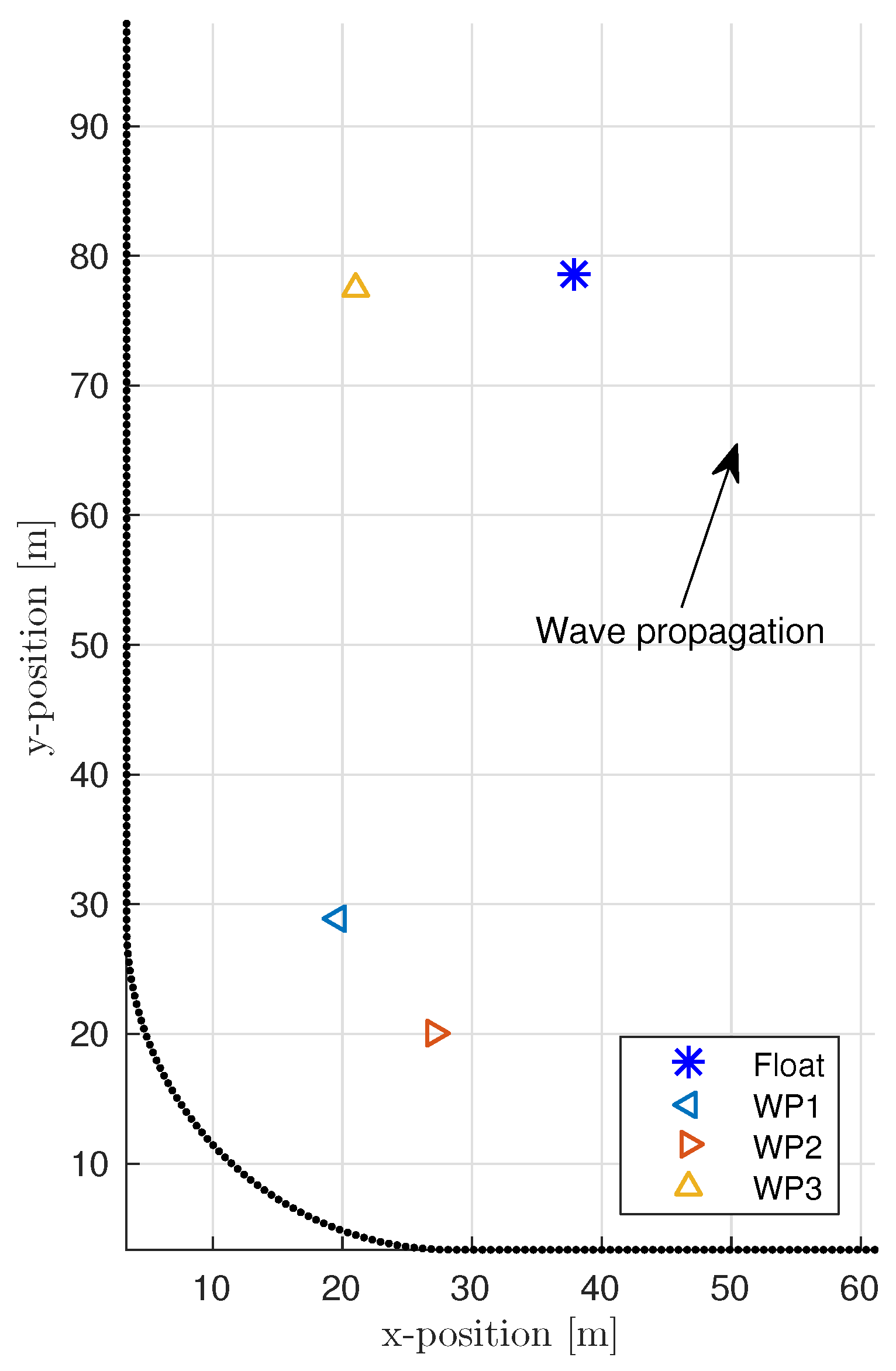
| Name | Type | x-Location (m) | y-Location (m) |
|---|---|---|---|
| Float | NA | 37.9 | 78.5 |
| WP1 | Capacitive | 19.7 | 28.9 |
| WP2 | Sonic | 27.2 | 20.1 |
| WP3 | Sonic | 21.0 | 77.4 |
| Test ID | Actuator Input | Actuator Freq. (Hz) | Actuator Gain | Wave Input | Wave Freq. (Hz) | Wave Gain |
|---|---|---|---|---|---|---|
| 010 | None | – | – | Pink | 1.00 | |
| 081 | White | 1.00 | None | – | – | |
| 082 | White | 1.50 | None | – | – | |
| 083 | White | 0.50 | None | – | – | |
| 084 | White | 1.25 | None | – | – | |
| 085 | White | 0.75 | None | – | – | |
| 086 | Pink | 1.00 | None | – | – | |
| 087 | Pink | 1.50 | None | – | – | |
| 088 | Pink | 0.50 | None | – | – | |
| 089 | Pink | 2.00 | None | – | – | |
| 090 | Pink | 0.75 | None | – | – | |
| 091 | Pink | 1.25 | None | – | – | |
| 105 | BLWN | 1.00 | BS | s | m | |
| 109 | Pink | 1.00 | Pink | 1.00 | ||
| 110 | Pink | 0.50 | Pink | 1.00 | ||
| 111 | Pink | 2.00 | Pink | 1.00 | ||
| 112 | Pink | 1.00 | Pink | 2.00 | ||
| 113 | Pink | 0.50 | Pink | 2.00 | ||
| 114 | Pink | 2.00 | Pink | 2.00 | ||
| 115 | Pink * | 2.00 | Pink | 1.00 | ||
| 116 | Pink * | 0.50 | Pink | 1.00 | ||
| 117 | Pink * | 1.00 | Pink | 1.00 |
© 2017 by the authors. Licensee MDPI, Basel, Switzerland. This article is an open access article distributed under the terms and conditions of the Creative Commons Attribution (CC BY) license (http://creativecommons.org/licenses/by/4.0/).
Share and Cite
Bacelli, G.; Coe, R.G.; Patterson, D.; Wilson, D. System Identification of a Heaving Point Absorber: Design of Experiment and Device Modeling. Energies 2017, 10, 472. https://doi.org/10.3390/en10040472
Bacelli G, Coe RG, Patterson D, Wilson D. System Identification of a Heaving Point Absorber: Design of Experiment and Device Modeling. Energies. 2017; 10(4):472. https://doi.org/10.3390/en10040472
Chicago/Turabian StyleBacelli, Giorgio, Ryan G. Coe, David Patterson, and David Wilson. 2017. "System Identification of a Heaving Point Absorber: Design of Experiment and Device Modeling" Energies 10, no. 4: 472. https://doi.org/10.3390/en10040472
APA StyleBacelli, G., Coe, R. G., Patterson, D., & Wilson, D. (2017). System Identification of a Heaving Point Absorber: Design of Experiment and Device Modeling. Energies, 10(4), 472. https://doi.org/10.3390/en10040472