Numerical Simulations of a VAWT in the Wake of a Moving Car

1
School of Marine Science and Technology, Northwestern Polytechnical University, Xi’an, 710072, China
2
Key Laboratory for Unmanned Underwater Vehicle, Northwestern Polytechnical University, Xi’an, 710072, China
*
Author to whom correspondence should be addressed.
Energies 2017, 10(4), 478; https://doi.org/10.3390/en10040478
Submission received: 23 January 2017
/
Revised: 7 March 2017
/
Accepted: 28 March 2017
/
Published: 3 April 2017
(This article belongs to the Section I: Energy Fundamentals and Conversion)
Abstract
:Wind energy generated from the wake of moving cars has a large energy potential that has not yet been utilized. In this study, a vertical axis wind turbine (VAWT) was used to recover energy from the wakes of moving cars. The turbine was designed to be planted by the side of the car lane and driven by the wake produced by the car. Transient computational fluid dynamics (CFD) simulations were performed to evaluate the performance of the VAWT. The influence of two main factors on the performance of the VAWT, the velocity of the car and the gap between the car and the rotor, were studied. The simulations confirmed the feasibility of this plan, and in the tested cases, the VAWT was able to generate a maximum energy output of 100.49 J from the wake of a car. The results also showed that the performance of the VAWT decreased with the velocity of the car, and the increased gap between the car and the VAWT.
1. Introduction
In recent years, the problem of fossil fuel resources and worldwide climate change are becoming more and more serious due to the rapid development of industrial economies and the fast growth of the world’s population. Most countries, especially developing countries, are facing the issue of an increasing demand for a limited supply of fossil fuel resources. As a result, worldwide interest in using renewable energy, such as wind energy, solar energy and hydrokinetic energy, to generate electricity, has risen in the past decade.
The Chinese government views highway construction as an important strategy for stimulating economic growth, and has built a nationwide network of highways. By the end of 2015, the highway mileage of China reached 123,500 km [1], and this number will keep increasing. According to dynamic monitoring data of the highways in 23 Chinese provinces, the total highway traffic flow was 516 million in July 2016 [2]. High-speed vehicles moving on highways produce strong disturbances to the air and transmit energy to the wake in the form of localized wind energy. The potential of the localized wind energy is high, considering the large amount of mileage and traffic flow that occurs. The idea of recovering energy from the wakes of vehicles has previously been proposed in several studies. Taskin et al. designed a combined solar and wind system to be planted in the median strip of highways, which uses a multi-stage Savonius rotor to generate power from the wind produced by cars [3]. Krishnaprasanth et al. designed a maglev turbine for highway wind power generation [4]. The above two studies are still at the design process, and no theoretical, numerical or experimental analysis has been given. While in the prototype stage, a Savonius turbine [5] and a hybrid wind turbine composed of a Darrieus rotor and a Savonius rotor [6,7] were designed and tested. These prototype studies showed the feasibility of using wind turbines to generate power from the wakes of moving vehicles. However, these tests are quite simplistic and no additional information about the wake field was given; also the mechanism of the interactions between the car wake and the rotor was unclear.
It should be noted that in all the above studies, vertical axis wind turbines (VAWTs) were utilized, rather than horizontal axis wind turbines (HAWTs). This is because the wind on both sides of the rotor proceeds in opposite directions, due to the opposing motion of vehicles, and the opposite aerodynamic forces driving the rotor. VAWTs have the advantage of easy self-start, and can operate at low wind speeds. Comprehensive studies have been done to evaluate and enhance the performance of VAWTs. The Darrieus turbine is one of the best-known VAWTs, which has three or four straight airfoils to create lift, and is the most efficient type of VAWT. Considerable effort has been made to model the dynamic forces on the Darrieus turbine [8,9]. The Darrieus turbine has also been studied extensively using CFD methods to optimize performance [10,11]. Variable pitch control mechanisms [12] and twisted blades [13] have been adopted to further improve starting torque and efficiency, and to deduce shaking of the Darrieus turbine. Although the two-dimensional CFD method is usually chosen for the simulations for less grids and a shorter simulation time, the three-dimensional CFDs studied have been accurately characterized for flow around the tip and the arm [9,11,14,15]. Savonius wind turbines have a lower efficiency compared with Darrieus types, but studies have shown that they have higher starting torque, good starting performance, and the ability to operate under complex turbulent flows [16]. The Savonius turbine has been studied experimentally and numerically to examine the effects of various design parameters, such as the rotor aspect ratio, the overlap, the number of buckets, the rotor endplates, and the influence of bucket stacking [17,18,19]. In addition, some researchers have worked to enhance the Savonius turbine performance by changing the structure of the turbine. Kamoji et al. studied the aerodynamic characteristics of a modified Savonius turbine with helical blades [20]. Golecha et al. placed a guide vane in front of the turbine to deflect flow for the returning blade [21]. Kacprzak et al. studied the performance of modified turbines with spline-type and Bach-type blades, and an increment of 16% in the efficiency was found in the case of using spline-type blades [22]. Tian et al. studied the performance of the Savonius turbine with new blades, including elliptical blades [23], and blades derived from the Myring Equation [24].
In this study, a VAWT is used to recover energy from the wake of moving vehicles. CFD simulations are performed to evaluate the performance of the turbine under different working conditions. The effects of the vehicle velocity, and the gap between the vehicle and the rotor are considered.
2. Model Simplification
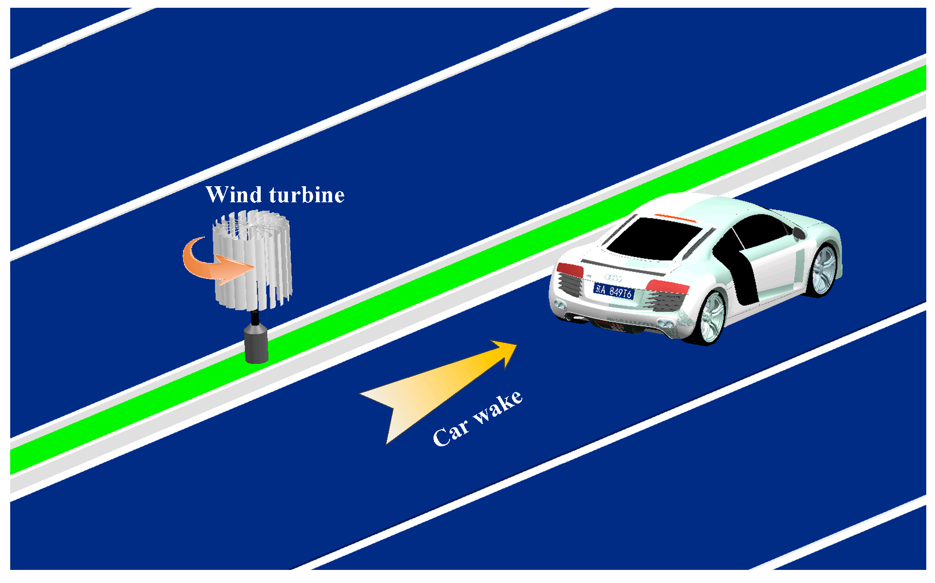
The VAWT is designed to be placed on the medians of the highway, therefore the wind on both sides of the median will contribute to the output of the turbine, as shown in Figure 1. This study only considers the situation for a single car passing by the turbine; more complex situations, such as multi-cars from one side and cars from both sides, will be studied later. Considering the complexity of the geometries and mesh, and the resultantly long computation time, a simplified two-dimensional model was chosen for the simulations. In the model, the side flow in the vertical direction was ignored. Studies have proved that the two-dimensional model can predict the performance of VAWTs with good accuracy [23,24]. Although this simplification may cause some inaccuracy, it is a good start for this study, and future research may consider the three-dimensional models for study.
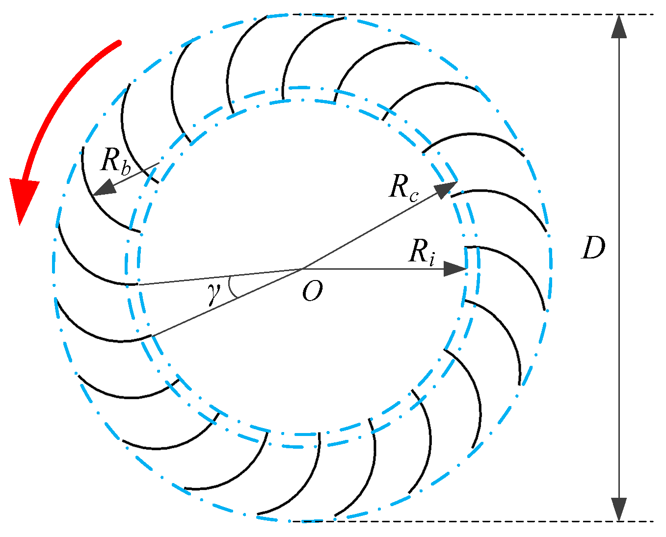
The performance of the rotor will determine the overall performance of the highway energy recovery system. Optimization studies on common VAWTs, like Savonius and Darrieus, have been done comprehensively. However, the bi-directional flow condition on the highway is different from common uniformed wind field, therefore a common Savonius or Darrieus rotor may not be the best choice for use. Common Savonius and Darrieus rotors have only two or three blades, and the aerodynamic forces of the rotor are very sensitive to the azimuth angle. In this paper, a Bánki wind turbine was used (Figure 2) [25]. The 20-bladed design makes this turbine more stable when wind direction and velocity change. The main geometric dimensions of the turbine are shown in Table 1. The car model considered in this paper was simplified as a two-dimensional shape composed of a rectangle and a semicircle, with a general size of 1.8 m × 4.5 m.
This study focused on evaluating the performance of the rotor in the wake of a moving car. Two key factors, the velocity of the car, v, and the gap between the car and the rotor, d, will influence the performance of the rotor, and are considered. The simulation cases are listed in Table 2. For each case listed in Table 2, simulations are carried out at rotor rotation velocities, ω, varying from 1 rad/s to 6 rad/s.
3. Numerical Method
The commercial CFD code FLUENT v15.0 was used to solve the incompressible Reynolds-averaged Navier-Stokes (RANS) equations using a second-order-accurate finite-volume discretization scheme. The shear stress transport (SST) k-ω turbulence model was selected to model the turbulence terms in the RANS equations.
3.1. Computation Domains and Boundary Conditions
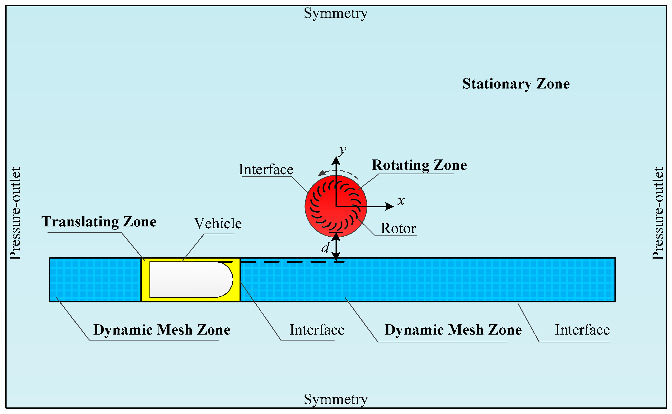
Figure 3 presents the computation domain and the boundary conditions. The computation domain was a rectangle with a length of 300 m and a width of 70 m, which was large enough to allow for the development of the flows. The turbine was placed in the center of the rectangular domain. The car moved horizontally and had a gap of d to the edge of the rotor. The position of the car was denoted as (x, y). The overall domain was split into several zones, including a rotor zone, a vehicle zone which is composed of a translating zone and two dynamic mesh zones, and a stationary zone containing the cells in the outer region. A sliding mesh method was used to realize the rotation motion of the rotor. For the vehicle, a combined sliding mesh and dynamic mesh method was used. In the simulation, the translating zone translated along the interfaces and the mesh in the adjacent dynamic mesh zones was updated at the end of each simulation step. The boundary conditions included pressure outlet boundaries on the left and the right, symmetry boundaries at the top and the bottom edges, no-slip walls on the surface of the rotor and the car, and interface boundaries at the overlap edges between the adjacent zones.
3.2. Mesh Generation
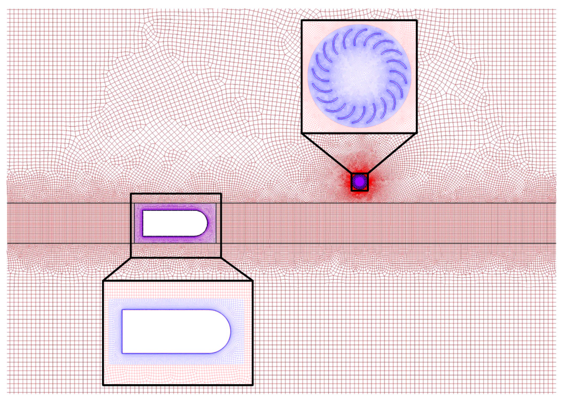
The dynamic mesh zones were meshed with structured grids and the other zones were meshed with unstructured grids. As shown in Figure 4, grid node density was higher in the rotor zone and the vehicle zone, than in the outer domain. Prism layer grids were extruded from the surfaces of the blades and the car to improve the grid quality. The height of the first prism layer was set so that the value for the first layer was below 10. Before the simulation, a mesh resolution study was performed to evaluate the influence of mesh resolution on the performance of the rotor. Several meshes were generated for the grid resolution verification at d = 1 m and ω = 1 rad/s. It is found that the results did not change much when the grids number exceeded 0.8 million. Therefore, the mesh with approximate 0.8 million grids was chosen for the following simulations.
3.3. Solution Sets
The initial position of the car was x = −45 m and the simulations ended when x = 117 m. The time step was set to 0.03 m/step, meaning that the car translated for 0.03 m in each step regardless of the car velocity. This time step was selected to be conservatively small, with the rotor rotating at a maximum angle of 0.69 m/step. A previous study used a time step of 1m/step and obtained good results [24].
3.4. Numerical Method Validation
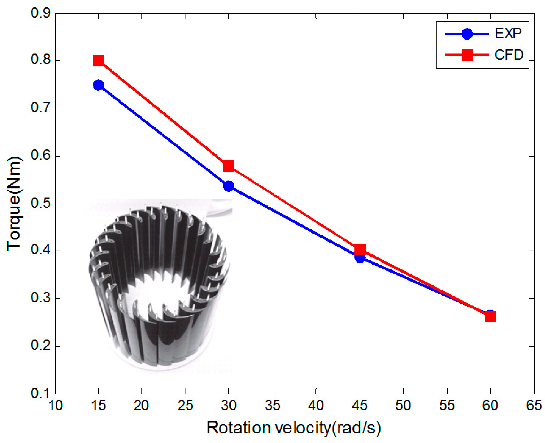
A validation study was conducted using a very similar wind turbine presented by Chiarelli et al. [26]. The validation simulations were performed using the two-dimensional CFD model by replacing the left boundary with a velocity inlet, and removing the car. The experimental rotor had a diameter of 0.25 m, a height of 0.21 m, and the testing wind velocity was 15 m/s. Figure 5 shows a comparison of the torque calculated using the CFD method with the experimental data, over a range of rotor rotation velocities. It was seen that the torques were in very good agreement with the experimental results, except for a slight overestimation at a rotation velocity of 15 rad/s, where the relative error is 6.8%.
4. Results and Discussion
4.1. Influence of the Rotor Rotation Velocity on the Performance of the Rotor (Case One)
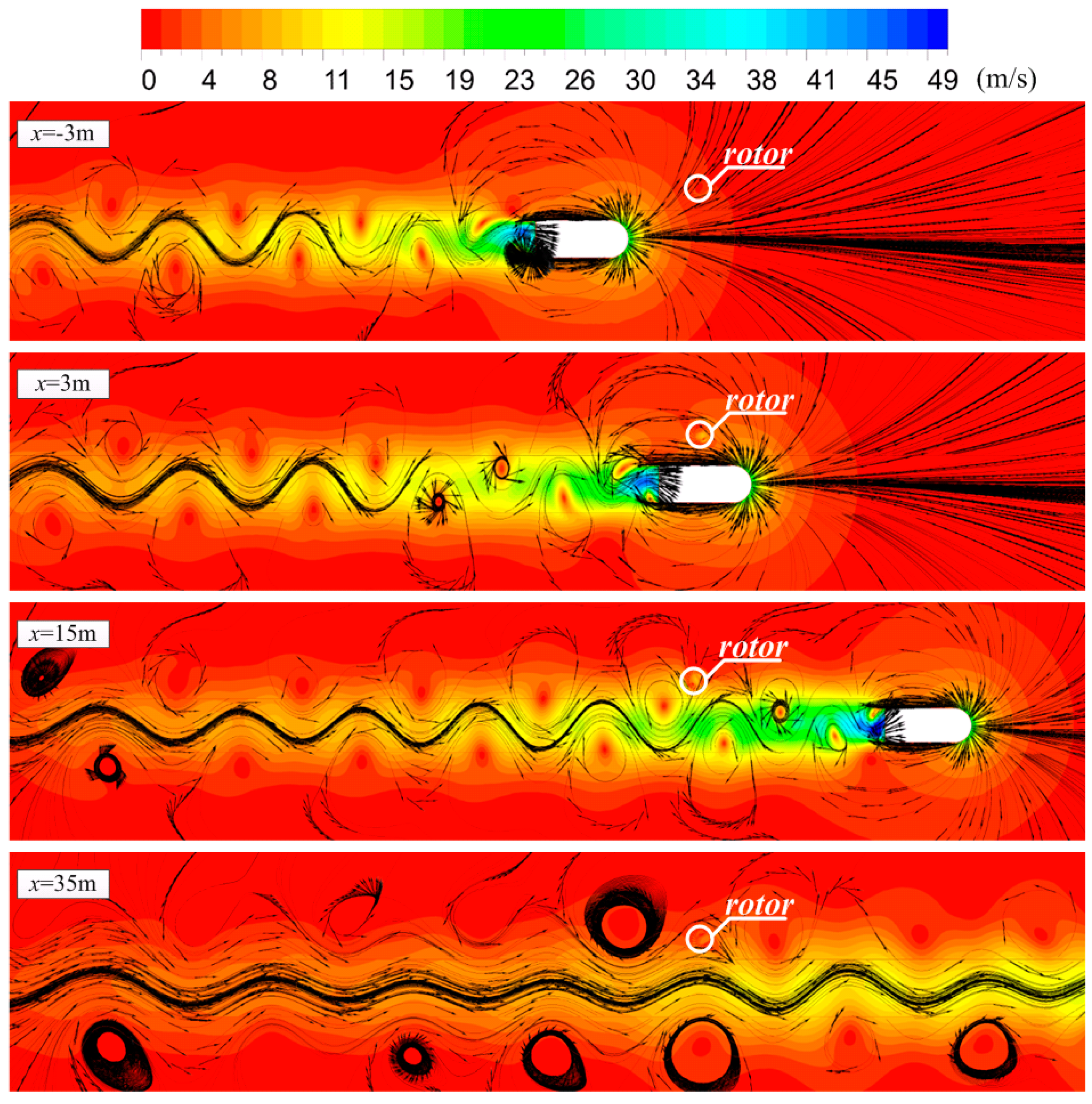
In order to understand the interactions between the car and the rotor, the contours of velocity and streamlines for Case One, ω = 4 and at different car positions are presented in Figure 6. Flows separated from the surface of the car and formed a repeating pattern of swirling vortices, which was similar to the Kármán vortex street. The vortices shed from the opposite sides of the car had different rotation directions, with those close to the rotor rotating counterclockwise.
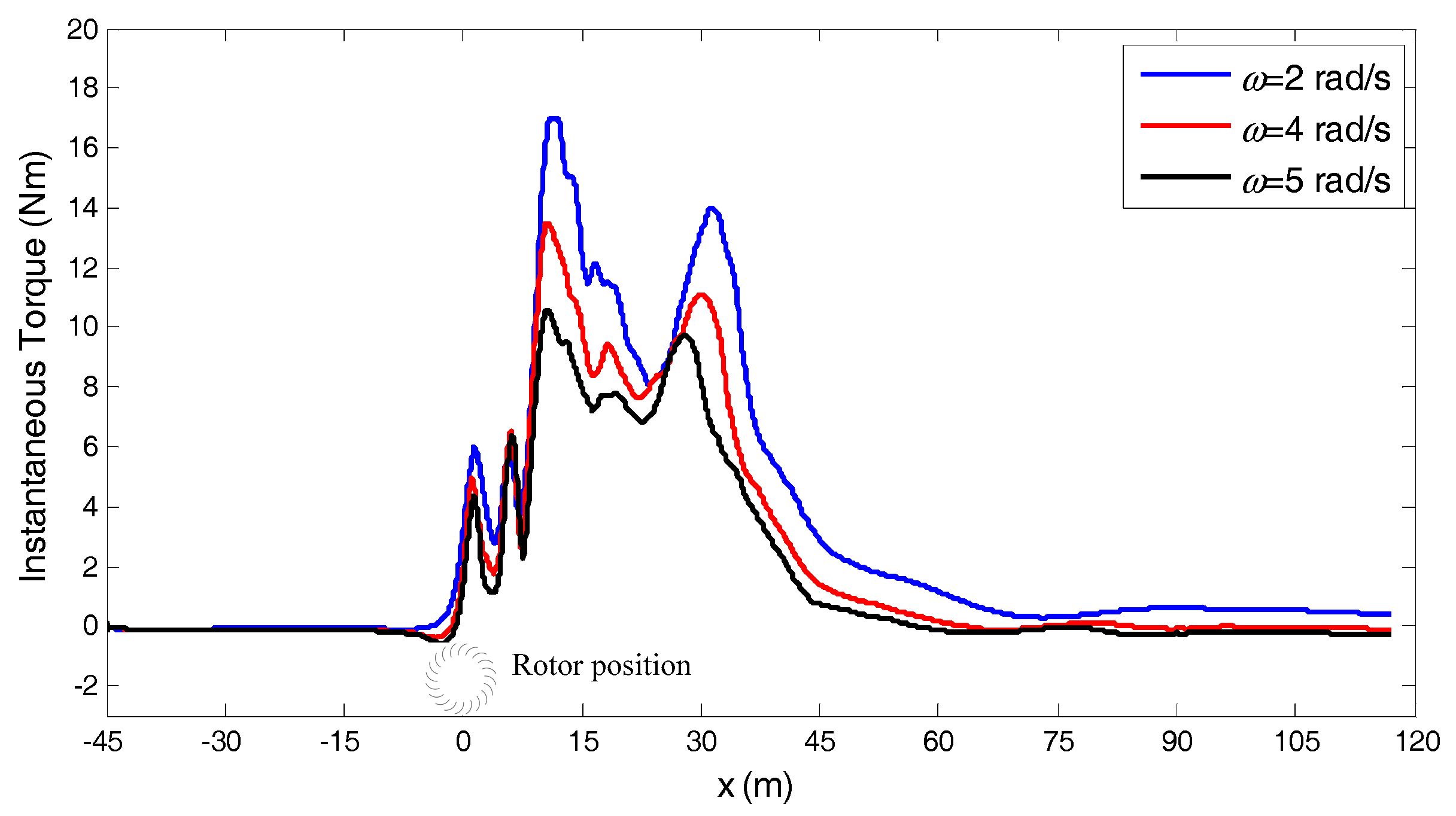
To investigate the influence of the rotor rotation velocity on the performance of the rotor, the instantaneous torques of the rotor in Case One, and for three rotation velocities, ω = 2, 4 and 5 rad/s, were plotted with respect to the position of the car, as shown in Figure 7. Positive torque was obtained mainly in the range of x = 0–60 m. When x < 0 m, the car was yet to reach the rotor and showed little effect on the torque of the rotor, so that the rotor rotated in nearly stagnant flow, and the torque was almost zero (x = −3 m in Figure 6). The torque then increased sharply and showed an obvious fluctuation between x = 0–9 m where the car just passed the rotor, and the velocity of the side flow changed dramatically (x = 3 m in Figure 6). The torque reached its maximum at x = 10 m, and remained at a relatively high value between x = 10–30 m; in this region the rotor was mainly influenced by the repeating swirling vortices separated from the car, and the torque of the rotor fluctuated (x = 15 m in Figure 6). As the car travelled further, the intensity of the wake grew weaker and the flow velocity around the rotor decreased, resulting in a drop in torque (x = 35 m in Figure 6). The curves of torque for different rotation velocities showed the same trend, except that higher rotational velocity resulted in a lower curve. Because the power of the rotor was the product of the torque and the rotation velocity, there would be an optimal rotation velocity which corresponds to the maximum power.
4.2. Influence of the Velocity of the Car on the Performance of the Rotor (Cases One to Four)
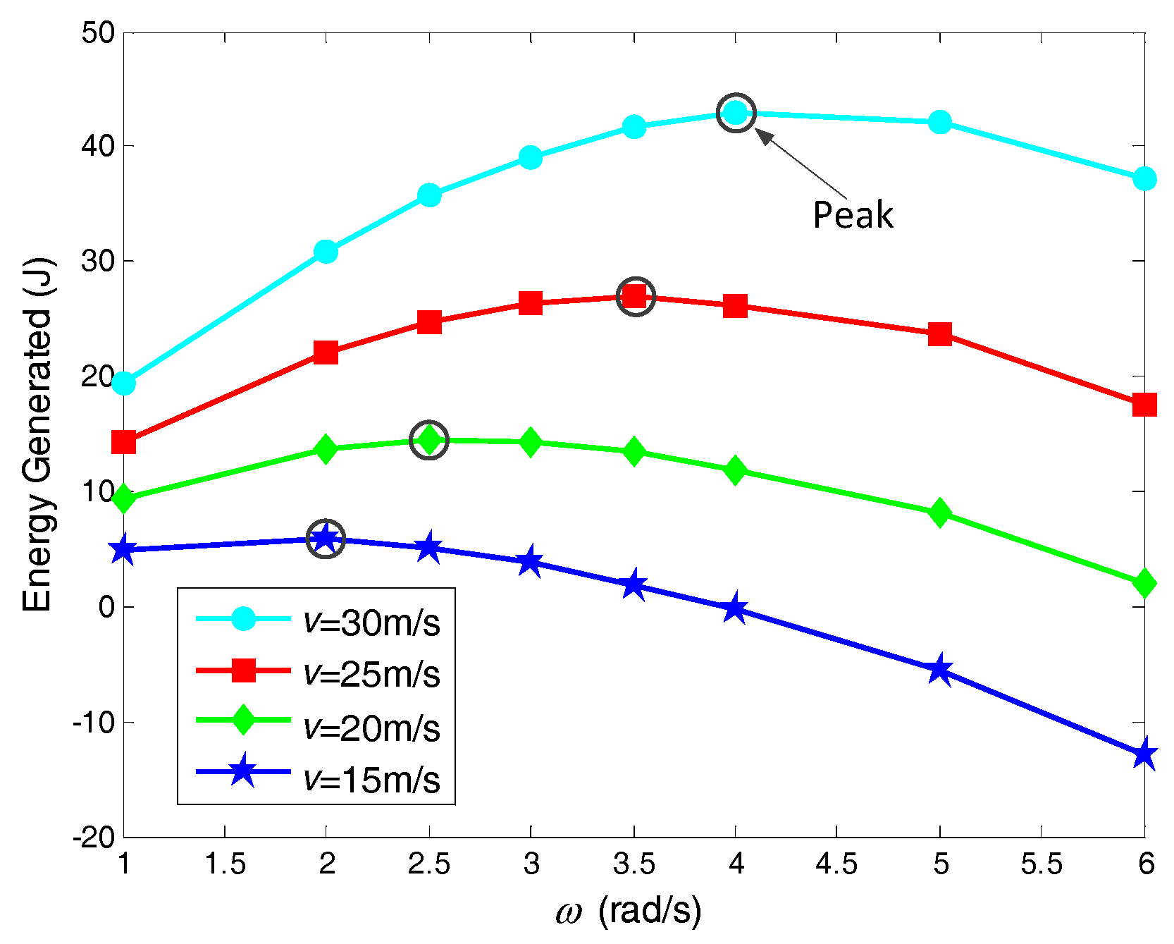
The rotor is expected to fit different working conditions after installation, and the first consideration is the velocity of the car. Cases One to Four were used to study the different influences of the car velocity. The total energy generated by the rotor from the wake of the car, E, which is the product of rotation velocity and the integral of the instantaneous torque in the whole range, was the most important indictor of the rotor. Figure 8 shows the E vs. ω curves of the rotor for four different car velocities, v = 15, 20, 25 and 30 m/s. Firstly, E increased with ω and then decreased after it reaches its peak. Secondly, the car with a higher velocity resulted in a higher E vs. ω curve and a larger ω where E reached its peak. This means that the rotor rotates faster and generates more power when the car moves faster.
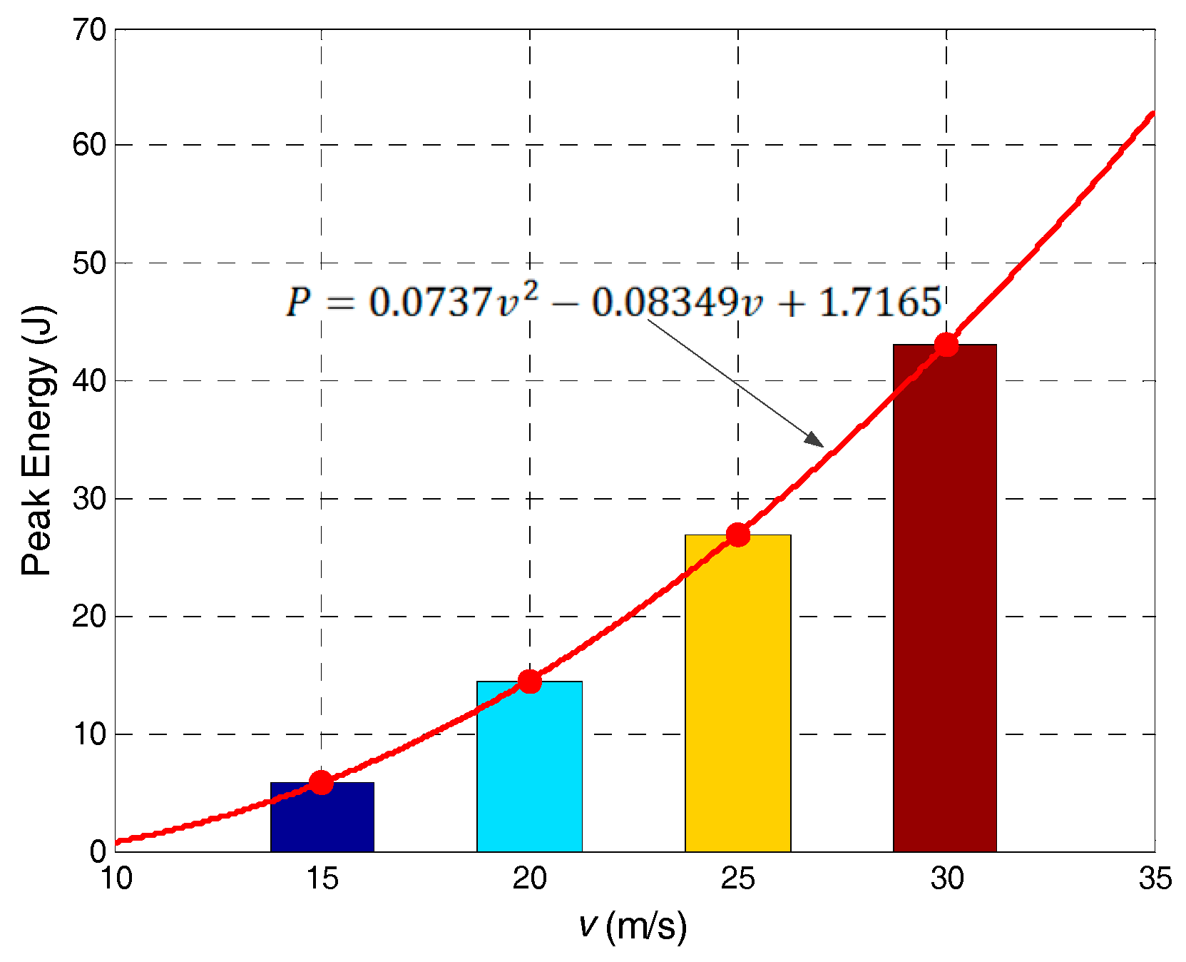
To quantitatively investigate the influence of the car velocity, Figure 9 shows the relationship between peak E and , along with a quadratic function that fit this data. This quadratic function is defined as . The rotor at 15 m/s predicted a peak E of 5.79 J (obtained at ω = 2 rad/s); while for the case of 30 m/s, the peak E increases to 43.02 (obtained at ω = 4 rad/s), and is 643% higher than the 15 m/s situation.
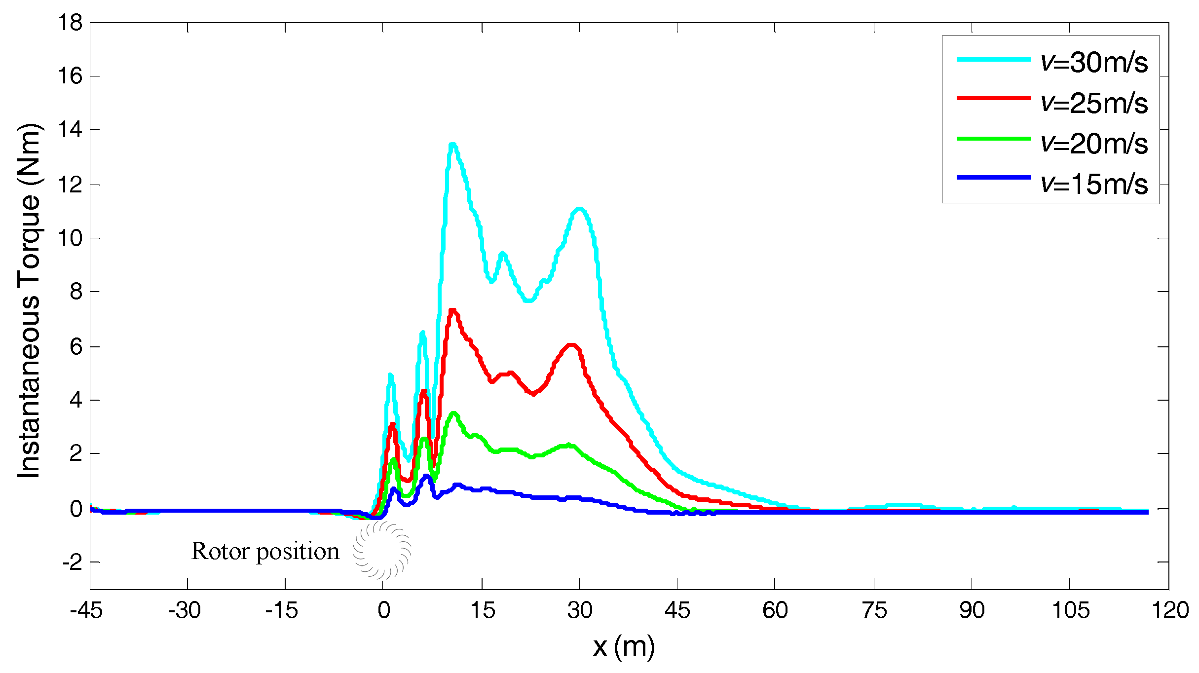
The instantaneous torques of the rotor at ω = 4 rad/s and at four car velocities, were plotted with respect to the position of the car, as shown in Figure 10. It can be seen that the curve of torque was entirely lowered with a decrease in the car velocity. Besides, the region of the positive torque was narrowed with the decrease of the car velocity. This illustrates that the car with a higher velocity has a stronger and longer effect on the torque of the rotor. The drop of torque finally led to the drop in generated energy.
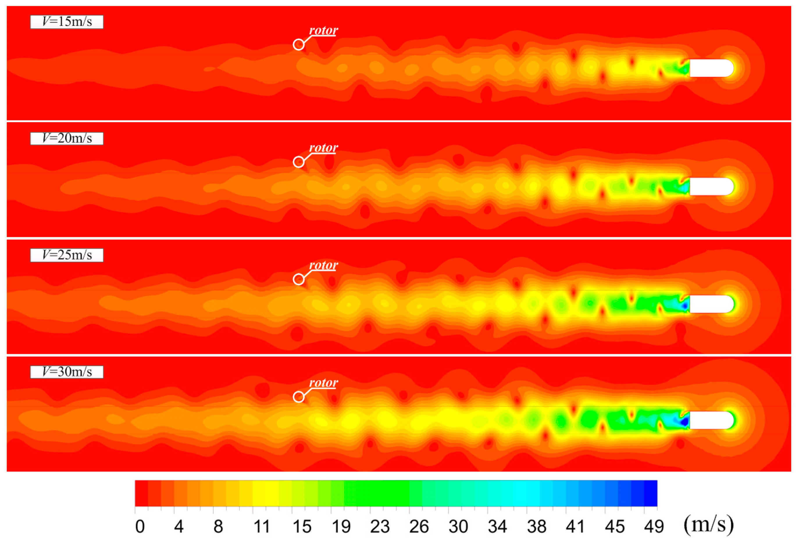
To explain the reason for the change of the rotor’s torque, the contours of velocity at x = 45 m are presented and shown in Figure 11. Both the length and the width of the car wake increased with the velocity, this means that the car has a larger region where the torque of the rotor is influenced. The velocity in the car wake also increased with the car velocity. A stronger wake contains more kinetic energy to drive the rotor. This explains why the curve of torque was higher at higher car velocities.
4.3. Influence of the Gap between the Rotor and the Car on the Performance of the Rotor (Cases One, Five to Seven)
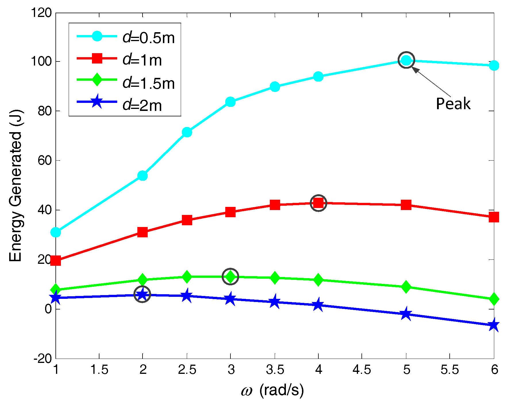
The gap between the car and the rotor, d, is another important factor that affects the performance of the rotor. Cases 1 and 5–7 were used to study the influences of the gap. Figure 12 shows the E vs. ω curves of the rotor for four different gaps, d = 0.5, 1, 1.5 and 2 m. It can be seen that the E vs. ω curve was entirely lowered with the increase of d, and the decrease in E was faster at a smaller d. The rotational velocity of the rotor corresponding to the peak E also decreased with a increase of d. This means that the rotor rotates faster and generates more power when the gap between the car and the rotor is smaller.
To quantitatively investigate the influence of the gap on the output power of the rotor, Figure 13 shows the relationship between the peak E and , along with a cubic function that fit this data. This cubic function was defined as . The peak E decreased with the increase of d. The rotor at 0.5 m predicted a peak E of 100.49 J (obtained at ω = 5 rad/s); while for 2 m/s, the peak E decreased to 5.57 J (obtained at ω = 2 rad/s), and was 94.46% lower than where 0.5 m.
The instantaneous torques of the rotor at ω = 4 rad/s and at four gaps, are plotted with respect to the position of the car and shown in Figure 14. It can be seen that the curve of torque was lowered with increasing d. Besides, the region of the positive torque was narrowed with increased d. This illustrates that the car passing the rotor with a larger gap has a weaker and shorter-lived effect on the torque of the rotor.
To explain the reason for the change of the rotor torque with the gap, the profiles of velocity in the wake of the car and upstream of the rotor (x > 0) for each of the four gaps are presented in Figure 15, where the car is moving at v = 30 m/s and at the position of x = 117 m.
The velocity was normalized according to , where is the upstream flow velocity and is the velocity of the car. The two axial distances, x and y, were normalized using the rotor diameter according to x/D and y/D, respectively. It can be seen that except for the curves at x/D = 90, the velocity profiles were approximately axisymmetric, with the axes of symmetry located in the middle of the car. At x/D = 90, it was close to the rear of the car, and the flow was greatly influenced by the wake vortexes of the car, and showed some fluctuation between −0.5 < y/D < 0.5. For the other cases, the velocity was higher near the axes of symmetry, and decreased gradually to zero away from the axes of symmetry. Because of the gap, the axes of symmetry were biased to the −y direction. For the four cases, the profiles of velocity are similar except that the offset of the axes of symmetry increased with d. Due to the bias of the velocity profiles, the velocity directly upstream of the rotor, as plotted between the two dashed lines in Figure 15, changed regularly with d. The larger the values of d, the smaller the velocities at all upstream distances.
The decrease of velocity means that less kinetic energy is generated from the wake, and the torque and the generated energy of the rotor is reduced.
4.4. Energy Balance Analysis
Although the rotor can extract energy from the wake of the car, it causes a blockage in the flow field of the car and this may increase the car drag. Therefore, the balance between the rotor generated energy and the energy of the car against the additional drag was investigated. Two cases were compared to show the relationship between the two kinds of energies. The first case was performed at v = 30 m/s, d = 1 m and ω = 4 rad/s, while the second one was the same except that the rotor was removed from the numerical model. The car drags of the two cases were then compared, as shown in Figure 16. Due to the periodically shed vortexes from the surface of the car, the drag changed periodically with nearly constant period and amplitude. No big differences were observed between the drags for the two cases in Figure 16a, this meant that the influence of the rotor on the drag of the car was weak. To more clearly show the changes, the drags are plotted between −10 m < x < 20 m together with periodic moving average curves. From the moving average curves, that the car drag increased slightly between −5 m < x< 15 m, this illustrates that the rotor causes additional drag on the car when it passes by the rotor, and the interacting region is limited to approximately 20D.
The averaged drags of the car were obtained by averaging the drag over the interacting region. The additional energy against drag was equal to the additional drag multiplied by the length of the interacting region. The results are listed in Table 3. The rotor caused an increase of 1.12 N in the car drag, resulting in an additional energy consumption of 22.40 J. The net energy generated in this process was the sum of the rotor energy and the additional consumed energy, and was equal to 20.62 J. This finding proves that although the car consumes additional energy, the rotor generates more energy from the car wake and the system is energy sustainable.
5. Conclusions
In this study, a VAWT was used to recover energy from the wake of a moving car. Transient CFD simulations were performed to study the performance of the turbine under different situations with two main factors considered, including the velocity of the car and the gap between the car and the rotor. An energy balance study was performed, proving the feasibility of this plan.
Important results of this research are as follows:
- (1)
- In the tested cases, the rotor was able to generate a maximum of 100.49 J energy from the wake of a car with d = 0.5 m, v = 30 m/s and ω = 5 rad/s.
- (2)
- The wake of the car was similar to the Kármán vortex street. The rotor was influenced by the repeating swirling vortices, and the torque of the rotor fluctuated significantly. Therefore, attention should be paid to the structure, strength, and design of the blades.
- (3)
- The performance of the rotor reduced with the velocity of the car, the reason being that a car with a smaller velocity generates a weaker wake, and the kinetic energy in the wake is reduced.
- (4)
- The performance of the rotor reduced with an increase in the gap between the turbine and the car, the reason being that the wake of the car is biased due to the gap and the velocity upstream of the rotor decreases with the increased gap.
The wake of a real car is more complex than a two-dimensional one because of vertical flow, therefore the CFD simulations in this study may have had some limitations due to the two-dimensional assumption. However, the two-dimensional simulations still proved the feasibility of the plan, and gave a good understanding of the interaction flows between the rotor and the vehicles. In order to make this plan a reality, some work needs to be done in the future:
- (1)
- Three-dimensional CFD simulations and field tests.
- (2)
- Tests on the influence of rotor types on the output power.
- (3)
- Tests on the performance of the turbine under the influence of multi-vehicles, and more complex highway conditions.
Acknowledgments
This research was supported by the National Science Foundation of China (Grant No. 61572404).
Author Contributions
Wenlong Tian and Zhaoyong Mao conceived the study and performed the simulations. Yukai Li reviewed and edited the manuscript.
Conflicts of Interest
The authors declare no conflict of interest.
References
- China’s Highway Mileage 2015. Available online: http://www.china-highway.com/Home/News/bencandy/id/112770.html (accessed on 31 March 2017).
- Traffic Flow on Highways in July 2016. Available online: http://www.chinahighway.com/news/2016/1044542.php. (accessed on 31 March 2017)).
- Taskin, S.; Dursun, B. Performance assessment of a combined solar and wind system. Arab. J. Forence Eng. 2009, 34, 217–227. [Google Scholar]
- Krishnaprasanth, B.; Akshaya, P.R.; Manivannan, L.; Dhivya, N.A. new fangled highway wind power generation. IJRASET 2016, 4, 31–34. [Google Scholar]
- Murodiya, R.; Naidu, H. Design and Fabrication of Vertical Wind Turbine for Power Generation at Highway Medians. Int. Eng. J. Res. Dev. 2016, 1, 1–10. [Google Scholar]
- Champagnie, B.; Altenor, G.; Simonis, A. Highway Wind Energy: Florida International University. Bachelor’s Thesis, Florida International University, Miami, FL, USA, 21 November 2013. [Google Scholar]
- Basilio, M.J.A.; Bernardo, J.T.; Cuya, J.B.L.; Luzano, G.C.C. Harnessing of Electrical Energy through Vehicular Air Drag on Highways for Lighting Load Applications. Bachelor’s Thesis, Mapúa Institute of Technology, Manila, India, May 2013. [Google Scholar]
- Deglaire, P.; Engblom, S.; Ågren, O.; Bernhoff, H. Analytical solutions for a single blade in vertical axis turbine motion in two-dimensions. Eur. J. Mech.-B/Fluids 2009, 28, 506–520. [Google Scholar] [CrossRef]
- Li, Y.; Calisal, S.M. Three-dimensional effects and arm effects on modeling a vertical axis tidal current turbine. Renew. Energy 2010, 35, 2325–2334. [Google Scholar] [CrossRef]
- Lain, S.; Osorio, C. Simulation and evaluation of a straight-bladed Darrieus-type cross flow marine turbine. JSIR 2011, 69, 906–912. [Google Scholar]
- Howell, R.; Qin, N.; Edwards, J.; Durrani, N. Wind tunnel and numerical study of a small vertical axis wind turbine. Renew. Energy 2010, 35, 412–422. [Google Scholar] [CrossRef]
- Schönborn, A.; Chantzidakis, M. Development of a hydraulic control mechanism for cyclic pitch marine current turbines. Renew. Energy 2007, 32, 662–679. [Google Scholar] [CrossRef]
- Gupta, R.; Biswas, A. Computational fluid dynamics analysis of a twisted three-bladed H-Darrieus rotor. J. Renew. Sustain. Energy 2010, 2, 4418–4422. [Google Scholar] [CrossRef]
- Alaimo, A.; Esposito, A.; Messineo, A.; Orlando, C.; Tumino, D. Sciubba E. 3D CFD analysis of a vertical axis wind turbine. Energies 2015, 8, 3013–3033. [Google Scholar] [CrossRef]
- Hasan, M.R.; Islam, M.R.; Hasan Shahariar, G.M.; Mashud, M. Numerical analysis of vertical axis wind turbine. In Proceedings of the 9th International Forum on Strategic Technology, Cox’s Bazar, Bangladesh, 21–23 Octomber 2014; pp. 318–321. [Google Scholar]
- Pope, K.; Dincer, I.; Naterer, G.F. Energy and exergy efficiency comparison of horizontal and vertical axis wind turbines. Renew. Energy 2010, 35, 2102–2113. [Google Scholar] [CrossRef]
- Akwa, J.V.; Júnior, G.A.D.S.; Petry, A.P. Discussion on the verification of the overlap ratio influence on performance coefficients of a Savonius wind rotor using computational fluid dynamics. Renew. Energy 2012, 38, 141–149. [Google Scholar] [CrossRef]
- Saha, U.K.; Thotla, S.; Maity, D. Optimum design configuration of Savonius rotor through wind tunnel experiments. JWEIA 2008, 96, 1359–1375. [Google Scholar] [CrossRef]
- Irabu, K.; Roy, J.N. Study of direct force measurement and characteristics on blades of Savonius rotor at static state. Exp. Therm. Fluid Sci. 2011, 35, 653–659. [Google Scholar] [CrossRef]
- Kamoji, M.A.; Kedare, S.B.; Prabhu, S.V. Performance tests on helical savonius rotors. Renew. Energy 2009, 34, 521–529. [Google Scholar] [CrossRef]
- Golecha, K.; Eldho, T.I.; Prabhu, S.V. Influence of the deflector plate on the performance of modified Savonius water turbine. Appl. Energy 2011, 88, 3207–3217. [Google Scholar] [CrossRef]
- Kacprzak, K.; Liskiewicz, G.; Sobczak, K. Numerical investigation of conventional and modified savonius wind turbines. Renew. Energy 2013, 60, 578–585. [Google Scholar] [CrossRef]
- Tian, W.; Song, B.; Mao, Z. Numerical investigation of a savonius wind turbine with elliptical blades. Proc. CSEE 2014, 34, 5796–5802. [Google Scholar]
- Tian, W.; Song, B.; Vanzwieten, J.; Pyakurel, P. Computational fluid dynamics prediction of a modified savonius wind turbine with novel blade shapes. Energies 2015, 8, 7915–7929. [Google Scholar] [CrossRef]
- Tian, W.; Song, B.; Mao, Z. A numerical study on the improvement of the performance of a banki wind turbine. Wind Eng. 2014, 38, 109–116. [Google Scholar]
- Chiarelli, M.R.; Massai, A.; Russo, G.; Atzeni, D.; Bianco, F. A new configuration of vertical axis wind turbine for a distributed and efficient wind power generation system. Wind Eng. 2013, 37, 305–320. [Google Scholar] [CrossRef]
Figure 1.
Schematic of the highway wind turbine.

Figure 2.
Cross section of the Bánki turbine.

Figure 3.
Computation domain and boundary conditions.

Figure 4.
Details of the computation mesh.

Figure 5.
Wind turbine used for the validation of the numerical method.

Figure 6.
Contours of velocity and streamlines for simulation Case One at different simulation times, rotor rotation velocity ω = 4 rad/s.
Figure 6.
Contours of velocity and streamlines for simulation Case One at different simulation times, rotor rotation velocity ω = 4 rad/s.

Figure 7.
Instantaneous torque of the rotor for Case One and at different rotation velocities (ω).

Figure 8.
Comparision of the generated energy for different car velocities (v).

Figure 9.
The peak wake-generated energy E with respect to the velocity of the car (v).

Figure 10.
Instantaneous torque of the rotor at rotor rotation velocity ω = 4 rad/s at four different car velocities (v).
Figure 10.
Instantaneous torque of the rotor at rotor rotation velocity ω = 4 rad/s at four different car velocities (v).

Figure 11.
Contours of velocity at position of car with respect to turbine x = 45 m, and at four car velocities (V).
Figure 11.
Contours of velocity at position of car with respect to turbine x = 45 m, and at four car velocities (V).

Figure 12.
Comparision of the generated energy for different gaps between car and turbine (d).

Figure 13.
The peak wake-generated energy (E) with respect to relative distance between car and turbine (d).
Figure 13.
The peak wake-generated energy (E) with respect to relative distance between car and turbine (d).

Figure 14.
Instantaneous torque of the rotor at ω = 4 rad/s and at four gaps (d).

Figure 15.
Profiles of velocity upstream of the rotor for different gaps (d).

Figure 16.
Variation of the car drag at v = 30 m/s, d = 1 m and ω = 4 rad/s, (a) global view; (b) zoom-in view for −10 m < x < 20 m.
Figure 16.
Variation of the car drag at v = 30 m/s, d = 1 m and ω = 4 rad/s, (a) global view; (b) zoom-in view for −10 m < x < 20 m.


Table 1.
Main geometric dimensions of the Bánki turbine.
| D (m) | Ri (m) | Rc (m) | Rb (m) | γ (°) | H (m) |
|---|---|---|---|---|---|
| 1.0 | 0.33 | 0.36 | 0.147 | 18 | 1.0 |
Table 2.
Simulation cases.
| Case | Car Velocity (m/s) | Gap between Car and Rotor (d) (m) |
|---|---|---|
| 1 | 30 | 1 |
| 2 | 25 | 1 |
| 3 | 20 | 1 |
| 4 | 15 | 1 |
| 5 | 30 | 0.5 |
| 6 | 30 | 1.5 |
| 7 | 30 | 2 |
Table 3.
Energy balance data.
| Case Description | Averaged Drag (N) | Additional Drag (N) | Interacting Region (m) | Additional Energy for Drag (J) | Rotor Energy (J) | Net Energy (J) |
|---|---|---|---|---|---|---|
| With rotor | 1218.88 | −1.12 | 20 | −22.40 | 43.02 | 20.62 |
| Without rotor | 1217.76 | 0 | 20 | 0 | 0 | 0 |
© 2017 by the authors. Licensee MDPI, Basel, Switzerland. This article is an open access article distributed under the terms and conditions of the Creative Commons Attribution (CC BY) license (http://creativecommons.org/licenses/by/4.0/).
Share and Cite
MDPI and ACS Style
Tian, W.; Mao, Z.; Li, Y. Numerical Simulations of a VAWT in the Wake of a Moving Car. Energies 2017, 10, 478. https://doi.org/10.3390/en10040478
AMA Style
Tian W, Mao Z, Li Y. Numerical Simulations of a VAWT in the Wake of a Moving Car. Energies. 2017; 10(4):478. https://doi.org/10.3390/en10040478
Chicago/Turabian StyleTian, Wenlong, Zhaoyong Mao, and Yukai Li. 2017. "Numerical Simulations of a VAWT in the Wake of a Moving Car" Energies 10, no. 4: 478. https://doi.org/10.3390/en10040478
Note that from the first issue of 2016, this journal uses article numbers instead of page numbers. See further details here.