Abstract
Tidal stream energy is a low-carbon energy source. Tidal stream turbines operate in a turbulent environment, and the effect of the structure between the turbine and seabed on this environment is not fully understood. An experimental study using 1:72 scale models based on a commercial turbine design was carried out to study the support structure influence on turbulent intensity around the turbine blades. The study was conducted using the wave-current tank at the Laboratory of Maritime Engineering (LABIMA), University of Florence. A realistic flow environment (ambient turbulent intensity = 11%) was established. Turbulent intensity was measured upstream and downstream of a turbine mounted on two different support structures (one resembling a commercial design, the other the same with an additional vertical element), in order to quantify any variation in turbulence and performance between the support structures. Turbine drive power was used to calculate power generation. Acoustic Doppler velocimetry (ADV) was used to record and calculate upstream and downstream turbulent intensity. In otherwise identical conditions, performance variation of only 4% was observed between two support structures. Turbulent intensity at 1, 3 and 5 blade diameters, both upstream and downstream, showed variation up to 21% between the two cases. The additional turbulent structures generated by the additional element of the second support structure appears to cause this effect, and the upstream propagation of turbulent intensity is believed to be permitted by surface waves. This result is significant for the prediction of turbine array performance.
1. Introduction
The existence of climate change is now unequivocal. Scientific data illustrates that the burning of fossil fuels has a role in the world’s climate. Particularly since the industrial revolution [1], the use of fossil energies has increased the level of atmospheric greenhouse gases including CO2, which reflect heat back towards the earth rather than allowing it to escape, thus leading to an increase in global temperatures. Following the production of a framework at the 2015 global climate change summit in Paris and the subsequent ratification by most major economies, an agreement to work to limit global temperature increase to below 2 °C [2] is now in place.
Electricity generation is the single largest source of greenhouse gas emissions both as a global average and in most countries. The move towards a future based on the generation of energy from lower carbon sources, avoiding the high CO2 emissions associated with electricity generation from fossil fuels, is therefore an important part of efforts to reduce greenhouse gas emissions and thus slow global temperature increase.
1.1. Renewable Energy
The burning of fossil fuels currently accounts for 67.4% of global electricity generation [3]. With global electricity demand continuing to grow, the replacement of fossil fuel-based electricity generation with renewable energy sources is crucial in order to reduce global CO2 emissions. A wide spectrum of renewable energy technologies exists, including marine energy.
1.1.1. Marine Energy
Marine energy describes technologies which generate energy from the oceans. These take three primary forms: (1) tidal energy, from the ebb and flow of tides due to the relative rotation of the earth and celestial bodies; (2) wave energy from the movement of waves ultimately derived from solar action at sea; and (3) ocean thermal current energy, commonly known as ocean thermal energy conversion (OTEC), generated from currents induced by thermal gradients in the oceans. In particular, tidal energy, which is the focus of the present paper, can be extracted either directly via tidal stream turbines or through the use of tidal lagoons or barrages.
None of the marine energy technologies illustrated in Figure 1. currently contribute any meaningful power to national networks in any country and all are considered immature technology, though it is worth noting that tidal barrages are in operation in South Korea, China, Canada, Russia, and France, where the 240-MW La Rance barrage has been in operation since 1966 [4]. However, the UK generates around 25% of its annual electricity demand from renewable energy, and this figure is rising annually. The development of prototype scale marine energy systems has been underway for some years, and many devices have already undergone extensive testing. As will be discussed later, a number of tidal stream turbine arrays are now in the design stage and are expected to be deployed within the next few years.
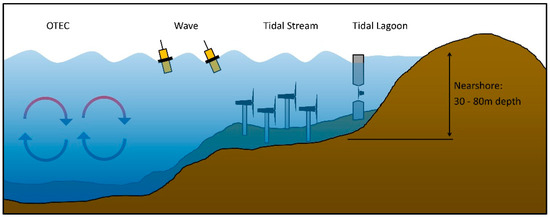
Figure 1.
Marine energy technologies: ocean thermal energy conversion (OTEC), wave, tidal stream and tidal lagoon.
1.1.2. Tidal Stream Energy
This paper relates to tidal energy extraction using tidal stream turbines. Tidal stream turbines extract power directly from the movement of tidal flows, generally in relatively shallow water in the nearshore region or inter-island channels. This feature differs them from other types of tidal energy capture such as barrages or tidal lagoons, which hold water to generate potential energy before releasing it to generate electricity.
Tidal stream energy has huge potential as a source of renewable electricity generation, with an estimated UK resource of 32 GW and the estimated potential to supply 20% of the UK electrical demand by 2050 [5].
In contrast to other renewable energy sources such as solar, wind and wave energy, which can be forecast on an annual scale, tidal energy has the advantage of being a more predictable resource. Tidal range and times can be calculated far in advance, and this offers the tantalizing prospect that in the future tidal power may be able to provide “base load” power, currently provided primarily by coal and gas-fired power stations. Though the resource at a single site is cyclical and therefore cannot deliver a constant power output, due to the differences in peak tide times, it has been suggested [6] that a number of interconnected generating sites offset around a coastline may be able to deliver a sufficiently constant output. Alternatively, large-scale energy storage systems could be used [7].
Potential locations for the extraction of tidal energy exist around the world. Examples of such sites include deep water sites around the Pentland Firth area to the north of Scotland, a number of potential sites in the Bay of Fundy and Vancouver Island straits, and some Mediterranean tidal sites around Sicily and Sardinia. All commercial developers of tidal stream energy envisage the deployment of multiple devices arranged in arrays, conceptually similar to the deployment of wind turbines in farms. Within arrays, the interaction of wakes and hydrodynamic effects is complex, and the turbulent characteristics of a wake generated by an upstream turbine are known to affect the performance of a subsequent downstream device.
1.2. Tidal Stream Turbines
Though a few alternative designs, such as oscillating hydrofoils [8], have been proposed, the vast majority of current tidal stream energy device designs are turbines [9]. A range of turbine designs have been proposed, including horizontal and vertical axis devices, and rigid, semi-rigid or floating mooring methods. However, the majority of tidal stream turbines are horizontal axis turbines with a rigid connection between the turbine unit and the seabed by a support structure. Our previous work, published in 2015 [10], studied the state of the art in tidal energy devices. We found that 18 tidal energy devices had undergone ocean tests, and that of these, 12 took the form of a horizontal axis turbine.
Due to the popularity of this form of device, the present work adopted a horizontal axis turbine as its subject. Due to its prevalence among such turbines which have been tested to prototype stage, we decided to consider only the rigid seabed-mounted design of support structure. A typical example of such a device, manufactured in this case by Andritz Hydro Hammerfest, is shown Figure 2. This 1-MW rated device measures 22 m from base to the center of the blades, and has a blade diameter of 23 m.
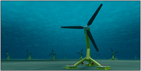
Figure 2.
Tidal stream turbine (Andritz Hydro Hammerfest).
1.3. Aims
A turbine and its support structure govern the hydrodynamic flow field around the device, including the downstream wake. Our previous [11] and other [12] works have studied the impact of turbine wake on the performance of downstream devices, and show that turbulent intensity (TI) in the downstream wake (i.e., potentially the incoming wake of a downstream device in an array setting) has an effect on performance. In some cases, increased ambient TI has been shown to reduce turbine performance [13], but some studies also suggest that increased ambient TI can yield small improvements in turbine performance [14]. In the case of a moored turbine, authors of [14] also describe the significant effect of increased TI on the displacement of the turbine from its original location, which is clearly an important consideration in array design. Studies in ship propeller design also suggest that in addition to absolute turbulent intensity, homogeneity is also important, and that the generation of a homogenous wake across a propeller leads to improved performance [15].
This work aims to understand the impact of different support structure designs on the performance of a device mounted on a support structure, as well as the impact on the resulting downstream wake. This will be undertaken through the use of two support structure designs in otherwise identical conditions.
1.4. Real Tidal Stream Case
Tidal array installation sites are typically located in channels of the order of 1 km to 5 km wide, with a typical water depth of between 35 and 80 m [16]. Sites with a mean spring peak tidal stream speed of 2 m/s or more [17] are potentially suitable for the installation of tidal energy devices, though numerous further considerations such as seabed type, distance from major port or grid connection, and tidal symmetry must also be considered.
In order to ensure replication of a suitable real case, this study used the proposed ScottishPower Renewables Sound of Islay site as its basis. The location of the site is shown in Figure 3.
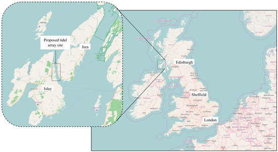
Figure 3.
Location of ScottishPower Renewables, Sound of Islay site (Map data © OpenStreetMap contributors, CC BY-SA).
The site lies between the islands of Jura and Islay in the Scottish Inner Hebrides, and the proposed array comprises ten devices in four rows across the channel, between the islands and the mainland. Although the development of the site is behind schedule and the proposed layout may change, the available data gives a useful insight into site conditions. Publically available data on the Sound of Islay site [18] and Andritz Hydro Hammerfest turbine [19] gives flow data in Table 1.

Table 1.
Data of Andritz Hydro Hammerfest turbine at the Sound of Islay site.
This data was used to correctly scale the turbine models used during water channel tests. Full details of the test cases and model design are given in Section 4.
In order to correctly replicate the real case during experimental work, realistic turbulence data was also required. Turbulent intensity describes the level of turbulence in a flow over a recording period by calculating the ratio of velocity fluctuation to mean velocity for the u (streamwise), v (cross-stream) and w (vertical) directions, then combining the result. For a given point in the velocity field, the root mean square of the velocity fluctuation time series, u′, is divided by the time-mean velocity, ū, over the same recording period, to give TI as a percentage. Turbulent intensity in the u direction, calculated from a sample of n recordings of velocity fluctuation u′ is given by:
1.5. Performance Analysis
A turbine of the type illustrated in Figure 2 has a rotational speed of 11 rpm at its rated power, at a flow velocity of u = 2.7 m/s. We herein calculate the tip-speed ratio (TSR or λ) as the ratio of the tangential rotational speed of a turbine to the flow speed in which it operates:
where ω is the rotational speed of the turbine in radians per second, R the blade radius in meters, and u the fluid flow speed in meters per second. Using the data in Table 1, the λ value of the Andritz Hydro Hammerfest turbines at the Sound of Islay site at rated power is 4.91. In this work we assumed λ = 5 for all scale testing.
When turbine performance over a range of λ values is known, λ is commonly plotted against the turbine power coefficient (CP) to give a turbine power curve. Power coefficient describes the ratio of the power generated by a turbine in a given flow case (PT) to the maximum theoretical power generated in the same sectional area and flow case, as given by PA. The maximum power in a stream of fluid of cross-sectional area A, velocity u and fluid density ρ is calculated using the following equation:
Thus giving Cp as follows:
The maximum Cp for any turbine is restricted to 0.593 by the Betz limit [20], though no commercial turbines are reported to have reached this value.
1.6. Support Structures
Two 1:72 scale support structure models were used in this study. The first structure, known as S1, was based on that of the Andritz Hydro Hammerfest turbine illustrated in Figure 2. In reality, the design uses three piled foundations to fix it to the seabed: one at the rear and two at the front. To the rear is a large support leg (20 mm in diameter at scale), which is angled forwards at 45°. A vertical support (34 mm in height at scale) is mounted on top of the angled support, giving an overall height support structure height of 250 mm. The lower part of the angled post is supported by two smaller arms which reach out to the sides. At scale these arms were 16 mm in diameter, 105 mm in length and their bases were 160 mm apart. A final section measuring 80 mm in length and 20 mm in diameter joined the main angled post to these front arms.
Our previous work suggested that the separation distance between the front face of a support structure and the swept area of the blades may directly impact the performance of an otherwise identical turbine [11], so a second support structure, S2, was designed to test this hypothesis.
With the aim of isolating this effect by minimizing other changes, the second structure was identical to the first, apart from the addition of a 25-mm diameter vertical post, located directly upstream (22.5 mm center-to-center) of the angled post. The separation distance between the support structure front face and the blade swept area, which previous work appeared to suggest may be important, was 42 mm for S1 and 20 mm for S2. The two support structure models as tested are illustrated in Figure 4.
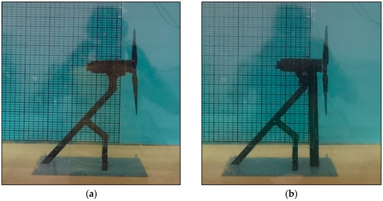
Figure 4.
Tidal turbine support structure model S1 (a); Tidal turbine support structure model S2 (b).
2. Results
2.1. Turbine Power
Mean blade power over 12,000 samples at λ = 5 was 0.163 W in the S1 case and 0.170 W in the S2 case, giving CP values in the two cases of 0.259 and 0.271. However, since the difference between these values is below the maximum power measurement error, no definite power output variation between the two cases can be assumed.
2.2. Upstream and Downstream Wake Tests
Data was recorded for three minutes during each test, giving 4500 velocity samples at 1 multiple of blade diameter D, 3D and 5D upstream and downstream, as illustrated in Figure 5.
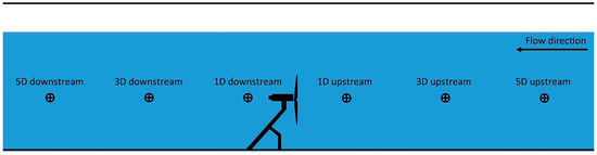
Figure 5.
Upstream and downstream Acoustic Doppler velocimetry (ADV) measurement locations during wake tests.
Due to processing requirements, 4096 samples were analyzed in each case, corresponding to 163.84 s of data. After processing using the filter developed by Cea et al. detailed previously [21], three-dimensional velocity data was used to calculate turbulent intensity at each location.
2.2.1. Velocity
Velocity data for support structures S1 and S2 at 1D, 3D and 5D upstream and downstream is shown in Figure 6. It was found that S1 and S2 case hub height upstream velocities at distances of 1D, 3D and 5D upstream were within 2% of each other. Downstream hub height velocities were very similar at 1D downstream, and exhibited around 2% variation at 3D and 5D downstream. These variations are within the range of error of the measurement equipment, so may be a function of experimental error rather than the performance influence of the support structure. Error calculations are given later.
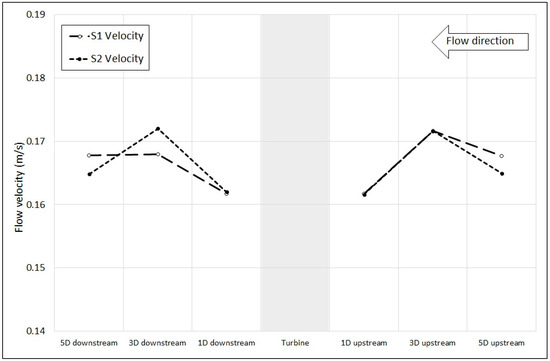
Figure 6.
Mean hub height streamwise velocity recorded at 1D, 3D and 5D upstream and 1D, 3D and 5D downstream of turbine mounted on S1 and S2 support structures (4096 samples at 25 Hz per point).
In order to investigate this further, velocity data was resampled into smaller data sets. Each 4096-point data set was split into four 1024-point data sets, as shown in Figure 7. The results which showed the greatest variation between the S1 and S2 cases in the global average case were the 3D and 5D downstream cases. The resampled data does not appear to support this, and illustrates that the observed global average variations were caused by large variation in the first quarter of the 5D downstream case, and the third quarter of the 3D downstream case.
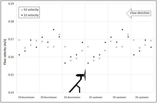
Figure 7.
Resampled hub height velocity recorded at 1D, 3D and 5D upstream and 1D, 3D and 5D downstream of turbine mounted on S1 and S2 support structures (1024 samples at 25 Hz per point).
Consequently, it appears that upstream and downstream velocity is unaffected by the differences in support structure between the S1 and S2 designs.
2.2.2. Turbulent intensity
From the velocity data illustrated in the previous section, turbulent intensity was calculated. This data, illustrated in Figure 8, showed that turbulent intensity in both the S1 and S2 support structure cases decreased between 5D and 3D upstream, then increased to its 1D upstream value. In the downstream region, turbulent intensity fell between 1D and 3D downstream, then rose slightly again at 5D downstream. The upstream and downstream data in both cases appears mirrored about the turbine, however the S2 case exhibits notably greater values of TI, with the difference between the two cases greatest closest to the turbine location.
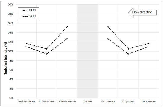
Figure 8.
Mean hub height turbulent intensity recorded at 1D, 3D and 5D upstream and 1D, 3D and 5D downstream of turbine mounted on S1 and S2 support structures (4096 samples at 25 Hz per point).
In order to validate the use of mean values in the data presented above, turbulent intensity data was also resampled to give four 1024-point data sets. This data is presented in Figure 9.
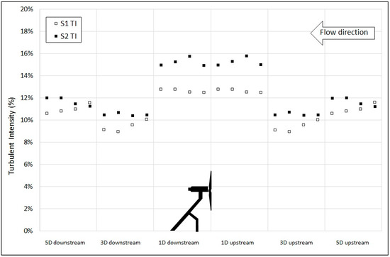
Figure 9.
Resampled hub height turbulent intensity recorded at 1D, 3D and 5D upstream and 1D, 3D and 5D downstream of turbine mounted on S1 and S2 support structures (1024 samples at 25 Hz per point).
This data appears to suggest that, in contrast to velocity results, turbulent intensity is affected by support structure, with the S2 design exhibiting greater TI values in both the upstream and downstream regions.
2.3. Blade Plane Tests
Velocity recordings using horizontally-mounted Acoustic Doppler velocimetry (ADV) unit were undertaken along a vertical line through the blade swept area (see Figure 16). With blades removed, a complete sample across the blade region at 0.25D (62.5 mm) spacing was recorded for the S1 and S2 support structure cases, as illustrated in Figure 10.
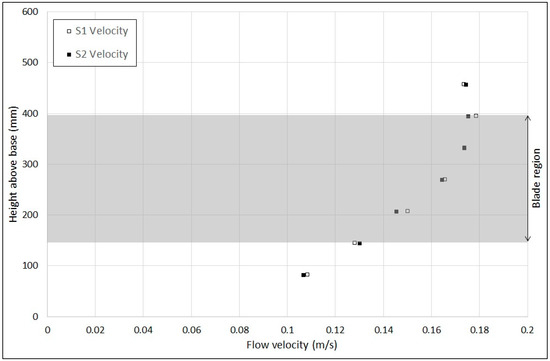
Figure 10.
Mean flow velocity recorded at blade plane. S1 and S2 support structures, nacelle in place, blades removed (4096 samples at 25 Hz per point).
This figure shows similar mean blade plane time-averaged flow velocities between the two support structures, though S1 does exhibit slightly higher velocities, particularly at the positions 207.5 mm and 395 mm above the channel base. However, variation between cases at these points is below the 2% error threshold.
Blade plane turbulent intensity is illustrated in Figure 11. This data shows a maximum variation of around 7% between cases, or a difference of around 0.5% TI, with S1 and S2 values at 332.5 mm above the base of 6.6% and 7.1% respectively. Turbulent intensity appears greater in the S1 case at heights above the turbine swept area, and greater in the S2 case over the blade-swept area, though it should be noted that this data was recorded without the blades in place and illustrates only the turbulent intensity generated by the support structure.
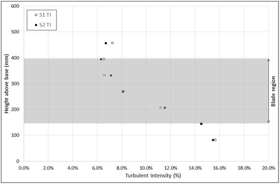
Figure 11.
Turbulent intensity recorded at blade plane. S1 and S2 support structures, nacelle in place, blades removed (4096 samples at 25 Hz per point).
To summarize the observed results, it appears that changing between support structures S1 and S2 has a negligible effect on flow velocity in both the upstream and downstream regions, as well as a negligible effect on velocity across the blade plane. Turbulent intensity does appear to be affected by the choice of support structure, with the S2 support structure generating greater hub height TI in the upstream and downstream regions (up to 5D in each case). Across the blade plane, TI is also affected by support structure, with the S1 case demonstrating greater intensity above the blade-swept region, and the S2 case generally greater within the blade-swept region.
3. Discussion
Experiments conducted on 1:72 scale models of a tidal turbine with two different support structure designs suggest that the variation in support structure design has an impact on the turbulent intensity upstream and downstream of the support structure, and over the water depth at the blade swept region.
The addition of a vertical upstream support post to a support structure based on a commercial design was found to increase turbulent intensity at 5D, 3D and 1D upstream by 6%, 12% and 21%, respectively, and downstream at 1D, 3D and 5D by 20%, 11% and 6%, respectively. In the blade region, TI variation of up to 7% between cases was recorded, with the addition to the structure of the upstream vertical post appearing to increase TI above the blade-swept region whilst decreasing it in the blade-swept region.
The measured increase in turbulence in the upstream and downstream regions due to the addition of the upstream vertical element to the support structure is the most significant experimental result of this work. It may be expected that the addition of the vertical post to the support structure would add a level of complexity to the downstream wake generated by the support structure, and thus may explain the additional turbulent intensity through the generation of more energetic turbulent structures. Perhaps the most notable aspect of the results of this study is the propagation of the turbulent intensity upstream. Although mean velocities are similar between the S1 and S2 cases, the increased TI suggests that the additional support structure element in the S2 case causes greater velocity variation in the region upstream of the S2 support structure. This upstream propagation of velocity is possible due to the flow conditions which allow surface waves to occur. The work described here was carried out with Froude numbers much lower than 1, meaning that the wave phase velocity or celerity is greater than that of the flow, allowing surface effects to propagate upstream. We believe that this effect transports the observed velocity fluctuation and TI upstream, giving the results seen in Figure 8.
It is important to note that the geometrical properties of the support structure play a role in the resulting turbulent environment. The resulting turbulent profile generated by any tidal turbine support structure should therefore be considered carefully, on an individual basis.
Limitations
Due to the limitations of working at scale, there are a number of effects experienced by real tidal stream turbines which are not replicated in this study. These include waves, bathymetry, and tidal ebb and flow directions. The last of these is of particular relevance to this study since tidal stream turbines must rotate between each tidal cycle to face the oncoming tide. Since the support structure is fixed to the seabed, the turbulent environment generated by the structure will be different during ebb and flow cases. This study only considered one flow direction.
A notable limitation to this study is the inclusion of only one turbine. As discussed earlier, tidal turbines are designed for installation in arrays, so the interaction of each turbine with the wake of upstream turbines must be considered. This effect has been studied in detail in our previous work [11], so is not included in this study.
Experimentally, the scale of the turbine models used imposed its own limitations on instrumentation and the measurement of performance data. Larger experimental facilities would allow testing at a greater scale, and for example may allow the use of generating (rather than driven) turbine models, removing the need for the vertical drive shaft. However, larger models and facilities bring their own inherent challenges, and additional expense.
4. Materials and Method
4.1. Water Channel
The work described herein was conducted in the wave-current water channel at the Laboratory of Maritime Engineering (LABIMA), University of Florence, Department of Civil and Environmental Engineering (www.labima.unifi.it). The channel is 37 m in length, with a width of 0.8 m and a maximum possible depth of 0.8 m. For this study, a water depth of 0.6 m was used, giving a water volume of 17.76 m3. This water depth was used with a turbine base to tip height of 394 mm (giving a height to depth ratio of 0.65, similar to the real case of a 30-m base-to-tip turbine in 48-m water depth, which yields a ratio of 0.625). A bulk flow rate of 74 L/s was used throughout.
Blockage ratio (the ratio of the frontal area of a blockage object to the cross-sectional area of the flow) is an important factor in the design of experimental models. Blockage ratios in previous experimental studies were found to range from 2% to 16.6% [22,23,24]. In these cases, blockage was calculated based on the total frontal area of the rotating turbine, including the entire swept area of the blades. In some cases, blockage calculated based on static frontal area (i.e., the frontal area of the blades was used instead of the swept area of the blades) was used, though those employing this method were in a minority. Arguably, at the relatively low rotational speed of a tidal turbine, a static blockage ratio may be appropriate, but due to the prevalence of the method in the literature, blockage ratios in this study were calculated using the more conservative swept area method. Blockage ratios for the work described herein were 10.2%. Blockage correction was not necessary in this study since results were used only for direct comparison between the two support structure cases, which have identical blockage ratios.
4.1.1. Measurement Equipment
Bulk flow conditions in the channel were measured using a magnetic flow meter (Danfoss MAGFLO MAG3100W and with MAG5000 output module, Danfoss A/S, Nordborg, Denmark) installed on the recirculation system in a pipe manifold measuring 250 mm in diameter. Water depth was monitored using ultrasonic distance sensors (Honeywell 943-F4V-2D-1C0-330E, Honeywell International Inc., Morris Plains, NJ, USA), positioned at 3.8 m, 18.5 m (1.65 m behind the installation position) and 35.5 m downstream from the inlet of the channel. The location of measurement equipment is given in Figure 12.
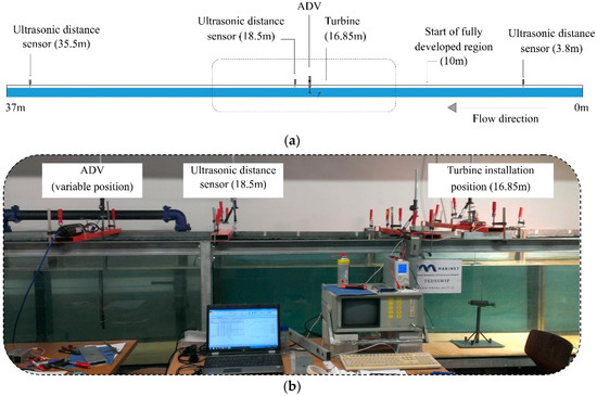
Figure 12.
Water channel schematic illustrating measurement locations (a); and photograph of central region (b).
The ADV system (model Nortek Vectrino) operated at a sampling frequency of 25 Hz and used a sample volume of 9.1 mm and transmit length of 2.4 mm. The 25 Hz recording frequency was chosen to ensure that all scales of flow structure would be captured, following the calculation of the turnover frequencies of the smallest and largest eddies in the flow. The predicted size of the Kolmogorov microscales for the planned experiments was 0.12 mm, giving a turnover time of 0.09 s and a maximum frequency of 11.1 Hz. Measurements at 25 Hz would therefore be able to capture the effects of even the most frequent eddy rotations, and sampling at a greater frequency than twice the maximum eddy frequency (i.e., greater than 22.2 Hz in this case) assured that the recorded data was not subject to aliasing. The turnover time of the largest eddies was calculated to be 5.3 s, giving a turnover frequency of 0.19 Hz.
All ADV velocity data recorded during this work was filtered using Velocity Signal Analyser software [25] and the cross-correlation filter developed by Cea et al. [21]. This filtering method was developed for use in turbulent open-channel conditions, and aims to retain the turbulent kinetic energy and power spectra characteristics of the original data whilst removing data spikes. The filter is based on the cross-correlation of u, v and w velocities and analyses of each sample independently (i.e., flow acceleration is not taken into account), allowing the detection of multiple consecutive spikes more easily than other filters.
After correlation of all data points within the set, replacement of spikes was undertaken. Three methods are recommended for the replacement of data: linear interpolation; the use of the last good value; or polynomial interpolation. The linear interpolation method was applied in the present study due to the simplicity of the method, though the maximum difference between resulting mean values in the data illustrated in the empty channel velocity profile (Figure 13) when using either of the other two methods was below 0.2%. The maximum difference between unfiltered mean velocity and filtered mean velocity in the data illustrated in this figure was 3.26%.
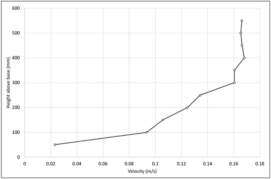
Figure 13.
Empty water channel time-averaged streamwise velocity profile at turbine installation location (flow conditions as described in Section 2).
4.1.2. Characterization
Prior to testing, characterization of the channel was carried out to verify the presence of a fully developed turbulent boundary layer. Time-averaged velocity profiles, each made up of eleven velocity recordings at 50-mm vertical intervals between 50 mm and 550 mm above the channel base, were recorded at multiple streamwise locations along the length of the channel.
At each streamwise position, 4500 samples (180 s at 25 Hz) were recorded at each of the eleven vertical locations. ADV specification and filtering methods were as described in the previous section.
Results indicate that the flow is fully developed from around 10 m downstream of the channel inlet (as highlighted in Figure 12), and a location downstream of this was therefore selected as the model installation location. For practical reasons, this was 16.85 m downstream of the inlet. The velocity profile recorded at this position is shown in Figure 13.
4.1.3. Similitude
The achievement of similitude in a scale model implies that the model is an accurate representation of reality, and is commonly defined by three criteria: geometric similarity, kinematic similarity, and dynamic similarity. The first criteria is met in this study through the use of scale models of a real tidal turbine, meaning that after scaling, the relative dimensions of the turbine and support structure elements are the same. Kinematic similarity describes the scaling of the flow pattern around an object, and is ensured by controlling the scaling of the flow field between the real and scale models, though by achieving geometric and dynamic similarity this criterion is automatically achieved.
Dynamic similarity describes the forces acting on the object, in reality and at scale, and requires that the forces at similar points on each should vary by a constant scale factor. The important forces to consider depend on the type of flow in question, but due to the low speed, low blockage ratio, free surface case considered here, the Reynolds number (Re) is the most appropriate. Clearly, real case Re values cannot be replicated at laboratory scale, but the requirement for a constant scale factor between similar points on real and scale cases was achieved, with a Reynolds number ratio of around 1200 between real and scale cases. Viscous effects can also be assumed to be negligible, since water channel Re values during this work were of the order of 40,000. Viscosity effects can be assumed negligible for Re values above 2000.
4.1.4. Turbulence-Generating Structures
The aim of the initial phase of testing was to ensure that the same level of ambient (i.e., at the test location without a turbine or support structure installed in the channel) turbulence was present in the water channel, as reported in real cases.
Turbulence data was not available for the Sound of Islay site, but a study by Thomson et al. [26] used Acoustic Doppler current profiling (ADCP) to measure velocity at a number of proposed tidal turbine installation sites in the Puget Sound, and thus calculated turbulent intensity. The study found mean TI values of around 11% at turbine hub height. In order to ensure correct scale replication of a real tidal installation site, our study aimed to match this value at the hub height of the scale turbine.
Water channel turbulent intensity was calculated, as described previously, from velocity data recorded using ADV positioned at 250 mm above the channel base. Initial values of TI were around 6%. In order to increase TI at the measurement location, two types of turbulence-generating structures were installed upstream: net structures occupying most or all of the cross-sectional area of the channel, and macro roughness on the channel base. The net structures included blocks built into semi-open walls and vertical bars (diameter 20 mm). Base-mounted macro roughness was generated using tubular structures measuring 27 mm in diameter and 100 mm in height.
A series of arrangements of these structures at various upstream locations were tested. Again using ADV, velocity was recorded and thus turbulent intensity calculated at hub height at the turbine installation location (though no turbine or support structure was installed during these tests). In each test, data was recorded for a minimum of 60 s, giving a minimum of 1500 velocity samples in each direction. These samples were then used to calculate fluctuation and mean velocities in each direction, and therefore the value of TI for the case. In data sets recorded for longer than 60 s, only 1500 samples were used. Results of these tests are given in Table 2.
Table 2.
Turbulence-generating structures and installation positions during Phase 1 tests.
Test 11 gave the closest result to the real case TI values recorded by Thomson et al, so this arrangement was used for all subsequent turbine tests. A full turbulent intensity profile (again without a turbine or support structure in place) recorded at turbine installation position is illustrated in Figure 14.
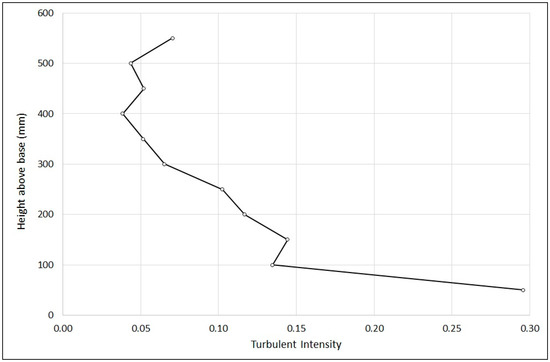
Figure 14.
Turbulent intensity profile at turbine location (case 11) without turbine.
4.2. Tidal Turbine Models
Having established a suitable turbulent regime within the water channel, the study set out to ascertain the influence of two turbine support structures on the performance of a turbine mounted on them.
4.2.1. Universal Turbine Model
A single turbine unit was used for all experiments, in order to ensure that the only change between cases was the support structure. The turbine blades were driven rather than allowing the turbine to rotate in the flow of water. This method has been employed in previous successful turbine model tests by others [23,27], and avoids problems associated with frictional losses in such small scale systems, which in a non-driven case can be greater than turbine-generated power.
The drive motor (Como 918 series with 1:100 gearbox, MFA Como Drills, Deal, Kent, UK) was mounted above the system, out of the water, and connected to the blades by a 90° gearbox in the nacelle by a vertical shaft extending through the top of the turbine body. Power calculation was as described in Section 4.2.2.
The nacelle design was based on the scaled geometry of a real turbine design, and has a length of 130 mm and a major diameter of 38 mm, tapering to 23 mm over the rear 25 mm of the length.
In order to minimize the overall cost of the project, a simple fixed pitch twin blade was used. The overall blade diameter was 250 mm, with each blade having a length of 118 mm, root and tip chord lengths of 17 mm and 13 mm respectively, and root and tip twist angles of 46° and 19°, respectively. Maximum chord length was 25.5 mm, at 50 mm from the blade root. Rotation direction was anti-clockwise when viewed from downstream. The turbine, blades and drive system connection are shown in situ in Figure 15.
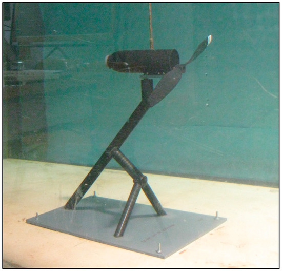
Figure 15.
Universal turbine model in situ during an S1 test.
4.2.2. Performance Measurement
A novel method, developed during previous work [11], was used to calculate the power and thus torque generated by the turbine blades during tests.
The turbine was driven using an electric motor during all tests. The power generated by an electric motor can be calculated from its voltage (V) and current (I), using the simple equation
P = I·V
By using a fixed voltage power supply (Rapid Electronics 1902, Rapid Electronics Ltd., Colchester, Essex, UK) and a current measurement module (Hobbycomponents ELC-05B, Hobby Components Ltd, Chesterfield, South Yorkshire, UK), these values were recorded during each test, thus giving the power required to drive the turbine in a given case.
In order to isolate the power generated by the turbine blade, and to exclude the portion of the supplied power required to overcome drive system and other losses, each test was conducted twice: initially with blades in place, and subsequently with the turbine blades removed. Power recorded during each test was recorded over the duration of the test, and the mean value calculated in each case, named PappB (motor power with blades) and PappNB (motor power without blades).
In order to set rotational speed ω and tip speed ratio λ, an optical encoder (Avago 500CPR, Avago Technologies U.S. Inc., San Jose, CA, USA) was mounted on the turbine drive shaft. Data from both the encoder and the current measurement module were recorded using a LabJack U12 data acquisition module at a frequency of 50 Hz. The same value of ω was used in both cases, but the required motor power to drive the turbine was lower in the case with blades, due to the power generated by the blades. By calculating the difference in motor power between the two cases, the blade-generated power (PB) could be isolated:
4.3. Experimental Methodology
The first phase of work in this study involved the use of turbulence-generating structures in the water channel to create a realistic turbulence environment for further studies. Results of these tests are given in Table 2. Following this initial study, a series of turbulence-generating structures giving a turbulent intensity of 11.1% at 250 mm above the channel base were used for all future studies.
The bulk of work in this study involved capture of simultaneous flow and turbine power recordings. Flow data was recorded using ADV, and turbine power data using the encoder and power measurement method described previously. A series of tests were carried out to find any differences between the two support structure cases.
4.3.1. Turbine Power
Power generated by the turbine in both the S1 and S2 support structure cases was measured. Flow velocity at the turbine hub height was 0.14 m/s, as shown in the velocity profile in Figure 13. To meet the required test tip speed ratio of λ = 5 the turbine was driven at a rotational speed of 5.6 rad/s (53 revolutions per minute). In both cases, motor current and rotational speed were recorded at 100 Hz, giving 12,000 data points for each measurement over each two-minute test.
4.3.2. Upstream and Downstream Wake Tests
The first set of tests were carried out with the aim of highlighting any differences between the upstream flow pattern and the downstream wakes between the two support structures. ADV data was recorded at three downstream (1D, 3D and 5D) and three upstream (1D, 3D and 5D) positions, in the horizontal center of the channel at turbine hub height (270 mm above channel base), as illustrated in Figure 5.
4.3.3. Blade Plane Tests
A second set of recordings were carried out using the ADV mounted horizontally to record flow data at a series of vertical positions on the swept plane of the blade. Tests were carried out both with and without the turbine blades in place. Data was recorded at seven positions in the case without the blades, and four positions in the case with the blades in place (since it was not possible to position the ADV unit close enough to record data in the center of the blades without the blades colliding with the ADV head). The locations used are illustrated in Figure 16.
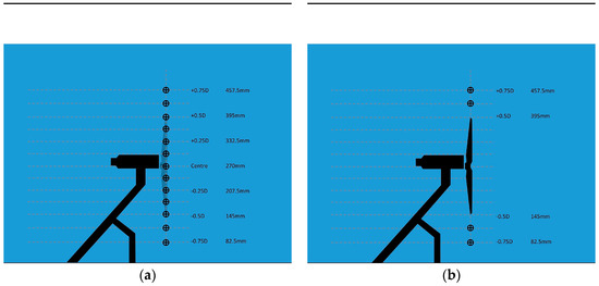
Figure 16.
ADV measurement locations during blade plane tests with blades (a); ADV measurement locations during blade plane tests with blades (b).
The water channel with turbulence-generating structures, measurement equipment and drive system, support structure and turbine all in place, is illustrated in Figure 17.
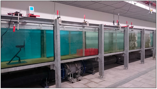
Figure 17.
Central section of water channel with turbulence-generating structures, turbine and support structure, and all measurement equipment in place.
4.4. Errors
4.4.1. Power Measurement Errors
When the method described in this paper is used, the deduction of PappB and PappNB in order to calculate the overall turbine-generated power PB removes the influence of any power losses within the motor and drive system, since these losses would be almost identical in the two cases and would therefore cancel out. However, there are two further sources of potential errors in turbine power measurement in this study.
The first would occur if additional bearing loadings were applied in one of PappB or PappNB cases but not the other, thus not being cancelled out during the calculation of PB. It is possible to imagine that the presence of turbine blades in the PappB case may cause such a situation, so an attempt to ascertain the influence of these loads on the power calculation was undertaken. Tests were performed to measure the minimum power required to drive the turbine with and without the blades in place, under otherwise identical conditions. These tests were carried out with the turbine and drive system installed in the water channel, but without water in the channel, by driving the turbine at a relatively high speed and then reducing the applied power until the minimum power required to sustain rotation was found, thus ensuring the measurement of dynamic loading. Variation in minimum power to achieve rotation of the turbine with and without blades was found to be 0.002% of PB. Since this value is below the threshold of accuracy of the measurement equipment, it was thus deemed negligible and system power loads were henceforth assumed to be identical in the two cases.
The second potential source of power measurement error stems from a misalignment of the turbine drive shaft. The potential for error due to this was estimated based on the maximum misalignment possible while a spirit level (used for driveshaft alignment) indicated that the shaft was vertical. When misaligned by 1 mm between top and bottom, the level indicator appeared at a glance to show that it was vertical, however when misaligned by 2 mm, the level indicator clearly showed a misalignment, giving a conservative maximum value of maximum misalignment of 2 mm.
In order to quantify this in terms of power applied to the turbine, motor position was moved 2 mm in the streamwise direction from a position used for previous experiments (and therefore believed to be correctly aligned). The power required to rotate the turbine with blades in place at the same speed as previously was found to be 9% greater. Total maximum error in power measurement was therefore assumed to be 10%.
4.4.2. Velocity Measurement Errors
ADV measurement accuracy is quoted by the manufacturers [28] as 1% in optimal conditions, though studies [29] have suggested that in sub-optimal conditions and near-bed regions, errors of the order of 5% can be seen. Signal-to-noise ratios (SNR) and correlation were monitored in this study to ensure velocity data accuracy. Mean SNR values were around 18 dB, and correlation in all cases was greater than 95%, suggesting that velocity measurement errors away from the near-bed region should not exceed 1%, or 2% in a worst-case scenario when results from two cases are used.
5. Conclusions
Turbulent intensity has numerous impacts on a tidal turbine, for example turbine performance, structural loading, and displacement of a moored turbine. The turbulent region generated around a tidal turbine is therefore of critical importance to a device developer seeking to achieve maximum performance at both device and array scale.
- Support structure design can have a significant effect on turbulent intensity in the region up to 5 rotor diameters downstream of a turbine.
- Support structure design can also have a significant effect on the region up to 5 rotor diameters upstream of a turbine, in cases where wave phase velocity is greater than flow velocity.
- Support structure design does not appear to have a significant impact on flow velocity upstream or downstream of the support structure.
As a concluding remark, it is worth pointing out that the presence of wind-waves in conjunction with sea currents is a rule rather than an exception. The effects arising from the superposition of wind-waves, in terms of the hydrodynamic changes and related effects on turbine performance, should be investigated. The study of this phenomenon is outside the scope of the present paper and will require further laboratory investigation in order to extend these results.
Acknowledgments
Access to the Laboratory of Maritime Engineering—LABIMA, of the University of Florence was funded by the MARINET FP7 EU Project (Marine Renewables Infrastructure Network for emerging Energy Technologies). The authors are grateful to this organization and to their respective institutions for their support.
Author Contributions
Stuart Walker conceived and designed the experiments; Stuart Walker and Lorenzo Cappietti performed the experiments, analyzed the data and wrote the paper.
Conflicts of Interest
The authors declare no conflict of interest.
References
- Edenhofer, O.; Madruga, R.; Sokona, Y.; Seyboth, K.; Matschoss, P.; Kadner, S.; Zwickel, T.; Eickemeier, P.; Hansen, G.; Schlömer, S.; et al. IPCC Special Report on Renewable Energy Sources and Climate Change Mitigation. Prepared by Working Group III of the Intergovernmental Panel on Climate Change; Cambridge University Press: Cambridge, UK; New York, NY, USA, 2011; p. 1705. [Google Scholar]
- Jahnz, A. Questions and Answers on the Paris Agreement. European Commission. Available online: https://ec.europa.eu/clima/sites/clima/files/international/negotiations/paris/docs/qa_paris_agreement_en.pdf (accessed on 17 October 2016).
- Key World Energy Statistics 2013; International Energy Agency (IEA): Paris, France, 2013.
- De Laleu, V. La Rance Tidal Power Plant: 40-Year Operation Feedback—Lessons Learnt. In Proceedings of the BHA Annual Conference, Liverpool, UK, 14–15 October 2009. [Google Scholar]
- UK Wave and Tidal Key Resource Areas Project: Summary Report; The Crown Estate: London, UK, 2012.
- Giorgi, S.; Ringwood, J. Can Tidal Current Energy Provide Base Load? Energies 2013, 6, 2840–2858. [Google Scholar] [CrossRef]
- Manchester, S.; Barzegar, B.; Swan, L.; Groulx, D. Energy storage requirements for in-stream tidal generation on a limited capacity electricity grid. Energy 2013, 61, 283–290. [Google Scholar] [CrossRef]
- Karbasian, H.; Esfahani, J.; Barati, E. Simulation of power extraction from tidal currents by flapping foil hydrokinetic turbines in tandem formation. Renew. Energy 2015, 81, 816–824. [Google Scholar] [CrossRef]
- Ng, K.-W.; Lam, W.-H.; Ng, K.-C. 2002–2012: 10 Years of Research Progress in Horizontal-Axis Marine Current Turbines. Energies 2013, 6, 1497–1526. [Google Scholar] [CrossRef]
- Howell, R.J.; Walker, S.; Hodgson, P.; Griffin, A. Tidal Energy Machines: A Comparative Life Cycle Assessment. Available online: http://eprints.whiterose.ac.uk/77080/ (accessed on 3 November 2016).
- Walker, S. Hydrodynamic Interactions of a Tidal Stream Turbine and Support Structure. In Mechanical Engineering; University of Sheffield: Sheffield, UK, 2014. [Google Scholar]
- Bahaj, A.; Molland, A.; Chaplin, J.; Batten, W. Power and thrust measurements of marine current turbines under various hydrodynamic flow conditions in a cavitation tunnel and a towing tank. Renew. Energy 2007, 32, 407–426. [Google Scholar] [CrossRef]
- Mycek, P.; Gaurier, B.; Germain, G.; Pinon, G.; Rivoalen, E. Experimental study of the turbulence intensity effects on marine current turbines behaviour. Part I: One single turbine. Renew. Energy 2014, 66, 729–746. [Google Scholar] [CrossRef]
- Pyakurel, P.; VanZweiten, J.; Dhanak, M.; Xiros, N. Numerical modeling of turbulence and its effect on ocean current turbines. Int. J. Mar. Energy 2017, 17, 84–97. [Google Scholar] [CrossRef]
- Sherbaz, S.; Duan, W. Propellor Efficiency Options for Green Ship. In Proceedings of the 9th International Bhurban Conference on Applied Sciences & Technology (IBCAST), Islamabad, Pakistan, 9–12 January 2012. [Google Scholar]
- Rolls-Royce. TGL DeepGen Brochure; Tidal Generation Limited: Bristol, UK, 2011. [Google Scholar]
- Tidal Stream Energy Review; Harwell Laboratory, Energy Support Unit, DTI: London, UK, 1993.
- ScottishPower Renewables. Sound of Islay Non Technical Summary; ScottishPower Renewables: Glasgow, UK, 2010; p. 17. [Google Scholar]
- Andersen, S.A. Development of ANDRITZ HYDRO Hammerfest’s Tidal Technology. In Proceedings of the 5th Bilbao Marine Energy Week, Bilbao, Spain, 23–25 September 2015. [Google Scholar]
- Betz, A. Windmills in the light of modern research. In National Advisory Committee for Aeronautics; NASA Technical Reoprts Server: Washington, DC, USA, 1928. [Google Scholar]
- Cea, L.; Puertas, J.; Pena, L. Velocity measurements on highly turbulent free surface flow using ADV. Exp. Fluids 2007, 42, 333–348. [Google Scholar] [CrossRef]
- Bahaj, A.; Myers, L. Report—Experimental Tests—Array Project; University of Southampton: Southampton, UK, 2008. [Google Scholar]
- Chamorro, L.P.; Hill, C.; Morton, S.; Ellis, C.; Arndt, R.; Sotiropoulos, F. On the interaction between a turbulent open channel flow and an axial-flow turbine. J. Fluid Mech. 2013, 716, 658–670. [Google Scholar] [CrossRef]
- O’Doherty, T.; Mason-Jones, A.; O’Doherty, D.; Bryne, C.; Owen, I.; Wang, Y. Experimental and Computational Analysis of a Model Horizontal Axis Tidal Turbine. In Proceedings of the 8th European Wave and Tidal Energy Conference, Uppsala, Sweden, 7–10 September 2009. [Google Scholar]
- Jesson, M.; Sterling, M.; Bridgeman, J. Desptking Velocity Time-Series—Optimisation through the Combination of Spike Detection and Replacement Methods. Flow Meas. Instrum. 2013, 30, 45–51. [Google Scholar] [CrossRef]
- Thomson, J.; Polagye, B.; Durgesh, V.; Richmond, M. Measurements of Turbulence at Two Tidal Energy Sites in Puget Sound WA. IEEE J. Ocean. Eng. 2012, 37, 363–374. [Google Scholar] [CrossRef]
- Stallard, T.; Collings, R.; Feng, T.; Whelan, J. Interactions between tidal turbine wakes: Experimental study of a group of three-bladed rotors. Philos. Trans. R. Soc. A 2013, 371, 20120159. [Google Scholar] [CrossRef] [PubMed]
- Nortek. Nortek Vectrino Lab Datasheet; Nortek A/S: Rud, Norway, 2013. [Google Scholar]
- Dombroski, D.; Crimaldi, J. The accuracy of Acoustic Doppler velocimetry measurements in turbulent boundary layer flows over a smooth bed. Limnol. Oceanogr. Methods 2007, 5, 23–33. [Google Scholar] [CrossRef]
© 2017 by the authors. Licensee MDPI, Basel, Switzerland. This article is an open access article distributed under the terms and conditions of the Creative Commons Attribution (CC BY) license (http://creativecommons.org/licenses/by/4.0/).