Surrogate Measures for the Robust Scheduling of Stochastic Job Shop Scheduling Problems

Abstract

This study focuses on surrogate measures (SMs) of robustness for the stochastic job shop scheduling problems (SJSSP) with uncertain processing times. The objective is to provide the robust predictive schedule to the decision makers. The mathematical model of SJSSP is formulated by considering the railway execution strategy, which defined that the starting time of each operation cannot be earlier than its predictive starting time. Robustness is defined as the expected relative deviation between the realized makespan and the predictive makespan. In view of the time-consuming characteristic of simulation-based robustness measure (RMsim), this paper puts forward new SMs and investigates their performance through simulations. By utilizing the structure of schedule and the available information of stochastic processing times, two SMs on the basis of minimizing the robustness degradation on the critical path and the non-critical path are suggested. For this purpose, a hybrid estimation of distribution algorithm (HEDA) is adopted to conduct the simulations. To analyze the performance of the presented SMs, two computational experiments are carried out. Specifically, the correlation analysis is firstly conducted by comparing the coefficient of determination between the presented SMs and the corresponding simulation-based robustness values with those of the existing SMs. Secondly, the effectiveness and the performance of the presented SMs are further validated by comparing with the simulation-based robustness measure under different uncertainty levels. The experimental results demonstrate that the presented SMs are not only effective for assessing the robustness of SJSSP no matter the uncertainty levels, but also require a tremendously lower computational burden than the simulation-based robustness measure.

1. Introduction

Job shop scheduling problem (JSSP) has been widely studied in the literature. However, in the real-world manufacturing environment, the scheduling performance of JSSP is affected by various uncertainties including the proficiency level of the workers, random machine breakdowns, the lack of tools or resources, the uncertain processing times, etc. [1,2]. In fact, most of these uncertainties result in stochastic processing times, thus named as a stochastic job shop scheduling problem (SJSSP) [3]. To keep up with a high profitable performance for a job shop, the scheduling needs to be robust against those inevitable disturbances.

Robust scheduling is an effective approach to deal with the uncertainties in the field of both machine scheduling and project scheduling. Herroelen and Leus [4] reviewed the techniques to cope with the uncertainties in project scheduling problems. Ouelhadj and Petrovic [2] summarized the methods on real-world scheduling in dynamic manufacturing environments. According to the literature, the robustness measures are mainly classified into two categories: quality robustness and solution robustness [4]. Quality robustness is often used to indicate the insensitivity of the scheduling performance under uncertainty in terms of the objective value, such as makespan, tardiness, while the solution robustness, also called stability, refers to the insensitivity of activity’s starting times to the uncertainty [5]. The improvement of quality robustness of SJSSP will reduce the risk of tardiness and increase the customer satisfaction. Therefore, we investigate the quality robustness that is defined by the expected deviation between realized makespan and predictive makespan [6].

Robustness evaluation is a critical process for robust scheduling. To appropriately assess the scheduling robustness, quantitative robustness measures are required to indicate the robustness performance of the evaluated schedules. The slack-based robust scheduling is a method based on the slack times or the insertion of additional idle times. It is widely used in the field of machine scheduling and project scheduling, which are mutually promoted. The slack-based robustness measures are divided into two categories. The first category allows the insertion of additional idle times or buffers that can be deemed as redundancy time, such as the literature by Ghosh et al. [7], Ghosh [8], Herroelen and Leus [9], Vonder et al. [10], Lambrechts et al. [11], Kuchta [12], Salmasnia et al. [13] and Jamili [14]. Although this approach is effective to improve the robustness, the insertion of idle time will inevitably increase the total cost of production. Furthermore, the strategies to determine the positions and units of the idle times or buffers are still the main difficulties as stated by Al-hinai and ElMekkawy [15]. The second category is to directly get the schedule solutions based on the neighborhood structure and/or the partially known uncertain information of the schedule without inserting additional idle times or buffers, such as the research by Goren and Sabuncuoglu [5], Leon et al. [6], Jensen [16,17], Artigues et al. [18], Ghezail et al. [19], Hazir et al. [20], Goren et al. [21], Xiong et al. [22] and Xiao et al. [23].

Stochastic scenario simulation-based measures also fall into the category without idle time insertion. Ahmadizar et al. [24] presented a simulation-based ant colony optimization algorithm to minimize the expected makespan in a stochastic group shop. In the study of Chaari et al. [25], a robust bi-objective evaluation function was developed to obtain a robust, effective solution that is slightly sensitive to data uncertainty. Wang et al. [26] proposed a two-phase simulation-based estimation of distribution algorithm for minimizing the makespan of a hybrid flow shop under stochastic processing times. However, the computational burden of simulation-based robust scheduling is usually unacceptable, thus a practical approach to improving the computational efficiency is to use the surrogate measure as an estimator and select an algorithm to optimize it [20].

The slack-based method is usually used in surrogate measures (SMs) to generate robust schedules [27]. Two types of slacks, i.e., total slack and free slack, have been widely studied in the literature for robust scheduling [20,22]. Total slack is defined as the difference between the earliest start time and latest start time of an activity while free slack is the amount of time that an activity can be delayed without delaying the start of the very next activity [28]. However, the available information on the uncertainty has seldom been considered in most of the literature. Leon et al. [6] proposed a surrogate measure using the mean of total slack, but the available uncertainty information was not fully utilized. Hazir et al. [20] proposed a surrogate robustness measure based on the potential critical operations, but the location of slack times had not been taken into consideration. Goren et al. [21] considered the variance of processing times on the critical path and developed an effective surrogate stability measure for the JSSP with machine breakdown and random processing times. However, the slack time and the non-critical operation were not considered. More recently, Xiong et al. [22] considered both the available uncertain information and the location of slack times, in which two effective SMs were proposed considering both the structure and the uncertainty information of the schedule for flexible JSSP under random machine breakdown. Due to the complexity of SJSSP, the existing SMs proposed for the project scheduling [10,20,28,29] and machine scheduling [6,21,22] are not well applicable for SJSSP. To the best of our knowledge, little research has been conducted on the robust scheduling of SJSSP by using SMs. In view of the wide range of industrial application of SJSSP in the field of discrete manufacturing, we focus on the SMs with the aim of providing the predictive schedules with satisfactory robustness and a lower computational burden.

To improve the accuracy of robustness estimation and reduce the computational burden of robust scheduling for SJSSP, we will utilize the probability distribution information of stochastic processing times and the structure of the schedule determined by the slack times to estimate the quantity of possible robustness degradation. Two SMs will be presented by analyzing the disturbances of critical operation set on the critical paths and non-critical operation set on the non-critical paths. The computational experiments demonstrate that the developed SMs are effective for the robust scheduling of SJSSP no matter if partial or all of the operations are uncertain. Therefore, the robust scheduling of SJSSP can be conducted by optimizing SMs and makespan simultaneously with a lower computational burden and a satisfactory robustness improvement.

The rest of this paper is organized as follows. Section 2 describes and analyzes the focused problem, and then the mathematical model of SJSSP is constructed. In Section 3, the existing SMs are discussed based on which two new SMs are suggested for the robust scheduling of SJSSP. A brief description of the HEDA is presented for the simulation experiments in Section 4. In Section 5, the effectiveness and the computational efficiency of SMs are verified by two simulation experiments. Finally, conclusions are given in Section 6 along with a description of the future work.

2. Mathematical Modeling

2.1. Problem Description and Analysis

A stochastic job shop scheduling problem (SJSSP) is the extended version of a JSSP by introducing some stochastic processing constraints such as stochastic processing time [3]. In this study, the SJSSP is described on the basis of JSSP: $n$ jobs processed on $m$ machines; each job has $m$ operations; the stochastic processing times $\xi T_{ij}$ of job $J_i$ at machine $M_j$ is assumed to follow a normal distribution $N({\mu }_{ij}, {\sigma }_{ij}^2)$; the operation’s process information is denoted by a vector $(M_j, {\mu }_{ij}, {\sigma }_{ij}^2)$. The following assumptions on JSSP are also used in the SJSSP: the setup time is included in the processing time and is not considered separately; a machine can only process one job at a time, and one job can only be processed on one machine at a time; each job can only be processed on one machine at most once; there are no precedence constraints between two jobs; the operations cannot be preempted; all machines are available at time zero.

In the literature on stochastic scheduling, various types of probability distributions for stochastic processing times have been studied, such as exponential distribution [3], normal distribution [30,31] and uniform distribution [25]. One method is to treat both the stochastic processing time and the scheduling objective as the stochastic variables, which aims at providing the processing ordering of the tasks on the machines with an expected optimization model. For example, Gu et al. [30] studied the SJSSP considering the processing times subjected to independent normal distributions with the aim of optimizing the expected makespan. The other direction is to firstly define an initial scenario of scheduling, then to deal with the uncertainties by imitating all of the possible scenarios. For example, Chaari et al. [25] studied the hybrid flow shop scheduling considering the processing times following a uniform distribution. An initial processing time scenario is obtained first. Then, the makespan and the initial scenario and the deviation of the makespan under all disrupted scenarios are minimized simultaneously.

In this study, we consider the processing time as a random variable and deal with it by using processing time scenarios, in which one scenario is denoted by a group of possible realized processing times. In the real-world job shop scheduling, a predictive guidance is vital to the production preparation to provide detailed directions on when to transmit the tools or the materials to the workstation, or on when to arrange operators to the corresponding machines prior to the execution of the scheduling. Therefore, we aim to provide a robust predictive schedule by firstly using the expected processing times as the initial processing time scenario, and then dealing with the disturbances caused by the stochastic processing times under the possible processing time scenarios. Simulation-based optimization is an effective way to solve the problem; however, it is very time-consuming, especially for the large-sized problems [20,22,26]. In order to speed up the optimization, inspired by the SMs of robustness that are designed for the robust scheduling of a flexible job-shop scheduling problem with random machine breakdowns [22], we put forward two SMs for SJSSP to estimate the robustness degradation by utilizing the available information of stochastic processing times and the structure of predictive schedule.

The railway execution strategy [32] that was adopted in the project scheduling is considered in this study, which means each activity will never start earlier than its planned starting time in the initial schedule. Since in the predictive schedule of SJSSP, the earlier completion of an operation will never affect the starting times of succeeding operations, we will only focus on the operations where processing times exceed the expected values. Additionally, the number of operations with stochastic processing times is random in the real-world manufacturing, so the SMs should be effective over all possible uncertain environments, regardless of whether partial or all the operations’ processing times are random. To describe the degree of the uncertainties, we define uncertainty levels (ULs) to represent the proportion of the operations those with stochastic processing times.

2.2. Mathematical Modeling of SJSSP

The purpose of robust scheduling of SJSSP is to generate the predictive schedule capable of absorbing the disturbances caused by the stochastic processing times when a right-shift reaction policy is adopted. Generally, the robustness measure (RM) can be estimated through Monte Carlo simulation to generate the possible processing time scenarios, shown as Equation (1):

$$RM\mathrm{sim}(S)=\frac{1}{L}{\displaystyle \sum _{l=1}^L[\xi C_{\max }^l(S)-C_{\max }^e(S)]}$$

(1)

where $l=1, 2, ..., L$ denotes the number of simulation replications of processing time scenarios, $RM\mathrm{sim}$ denotes the simulation-based robustness measure and $\xi C_{\max }^l(S)$ denotes the potential realized makespan of schedule $S$ under the $l\mathrm{th}$ simulation by sampling a potentially realized processing time scenario.

The studied SJSSP is described by a triplet proposed by Graham et al. [33]. Therefore, the problem is described as $J_m\left|\mathrm{SPT}\right|\eta C_{\max }^e+(1-\eta )RM$, where $J_m$ denotes the JSSP, $\mathrm{SPT}$ denotes the stochastic processing times, $C_{\max }^e$ denotes the makespan of the predictive schedule and $RM$ denotes the robustness measure. The robust scheduling model of SJSSP considering the predictive makespan and the robustness measure is shown as follows:

$$\underset{S\in \Omega }{\min }F(S)：F(S)=(1-\eta )C_{\max }^e(S)+\eta RM(S)$$

(2)

subject to

$$\begin{array}{l}\xi C_{ik}-\xi T_{ik}+M_0(1-a_{ijk})\ge \xi C_{ij}\\ i=1, 2, ..., n;j, k=1, 2, ..., m\wedge j\ne k;\end{array}$$

(3)

$$\begin{array}{l}\xi C_{hj}-\xi T_{hj}+M_0(1-x_{ihj})\ge \xi C_{ij}\\ i,h=1, 2,..., n\wedge i\ne h;j=1, 2, ..., m;\end{array}$$

(4)

$${\displaystyle \sum a_{ijk}}=1,\forall i, j, k\wedge j\ne k;$$

(5)

$${\displaystyle \sum x_{ihk}}=1,\forall i, h, k\wedge i\ne h;$$

(6)

$$a_{ijk}\in \{0,1\},\forall i, j, k\wedge j\ne k;$$

(7)

$$x_{ihj}\in \{0,1\},\forall i, h, j\wedge i\ne h;$$

(8)

$$\xi C_{ij}\ge 0,\forall i,j.$$

(9)

In the objective function as Equation (2), $\eta$ and $1-\eta$ denote the weight coefficients of robustness measure $RM$ (can be represented by RMsim and the SMs) and efficiency measure $C_{\max }^e(S)$, respectively, where $\eta \in [0,1]$. The inequality (3) represents the process constraints, which means the job $J_i$ has to be processed on the machine $M_j$ before being processed on the machine $M_k$. If this condition is satisfied, $a_{ijk}=1$, else zero. $M_0$ is a large enough positive number. The machine constraints are denoted by Inequality (4), which means the job $J_h$ has to be processed on the machine $M_j$ after job $J_i$, if this constraint is satisfied, $x_{ihj}=1$, else zero. Constraints (5) and (6) denote that one machine can only process one job at one time and one job can only be processed on one machine at the same time. While Constraints (7) and (8) state that the value of $a_{ijk}$ and $x_{ihj}$ can only be integer one or zero. The inequality (9) represents that none of the completion times of the operations can be negative.

3. SMs of Robustness for SJSSP

3.1. The Existing SMs of Robustness

To facilitate the description of the SMs, several definitions for SJSSP are given:

Definition 1.

Critical path (CP): The longest path composed of the operations where any delay in any operation would increase the makespan.

Definition 2.

Non-critical path (NCP): The paths constructed by all of the operations except for the operations on the critical path.

Definition 3.

Critical operation set: The operation set where any delay in any operation would increase the total makespan, denoted by ${\mathrm{O}}_{\mathrm{cp}}$.

Definition 4.

Non-critical operation set: The operation set in which all of the operations have total slack time, denoted by ${\mathrm{O}}_{\mathrm{ncp}}$.

Definition 5.

Disturbance absorption capability: The capability of a predictive schedule to absorb the disturbances caused by stochastic processing times by using slack times existing in the schedule structure.

A surrogate measure for evaluating the absorptive capability of a schedule was proposed based on the average total slack time in the research of Leon [6], which is rewritten as SM1:

$$SM1=C_{\max }^e-{\displaystyle \sum _{i=1}^n{\displaystyle \sum _{j=1}^{m}T{S}_{ij}}}/mn$$

(10)

where $T{S}_{ij}$ denotes the total slack time of operation $O_{ij}$.

The SMs that aim at providing an accurate estimation of the schedule robustness for the multi-mode project scheduling problem were investigated in the study of Hazir et al. [20]. In one surrogate measure, they define the activities that have total slacks ($T{S}_{ij}$) less than a certain percent ($\xi$) of the expected activity duration $({\mu }_{ij})$ as the potential critical activities (PCA), i.e., $\mathrm{PCA}=\{O_{ij}:T{S}_{ij}/{\mu }_{ij}\le \xi \}$. The delays in PCA are likely to result in delays in the project completion time. Schedules with fewer critical activities are preferred on the robustness. The measure of PCA can also be used in SJSSP because of the similarity of the two problems, which is named potential critical operations (PCO). Assuming the variance of SJSSP is known, the definition of PCA is revised to include the effect of the standard deviation, i.e., $\mathrm{PCO}=\{{\mathrm{O}}_{ij}:T{S}_{ij}/({\mu }_{ij}+{\sigma }_{ij})\le \xi \}$. Therefore, a new definition of SM2 is written as:

$$SM2=\left\{N_{\mathrm{pco}}/mn:O_{ij}\in {\mathrm{O}}_{\mathrm{pco}}\right\}$$

(11)

where $N_{\mathrm{pco}}$ denotes the number of PCO and ${\mathrm{O}}_{\mathrm{pco}}$ denotes the set of PCO, which includes all of the operations that satisfy the inequality $T{S}_{ij}/({\mu }_{ij}+{\sigma }_{ij})\le \xi$, and we set $\xi =0.25$ in this study.

Goren et al. [21] developed a surrogate stability measure to generate efficient and stable schedules for a job shop subject to processing time variability and random machine breakdowns. The variance of the realized completion time is estimated as the sum of the variances of the arc lengths that lie on the mean-critical path. Therefore, the expected delay of the realized completion times can also be estimated by the proposed measure. If there is more than one mean-critical paths, the one with the maximum total variance is selected. This surrogate measure is based on decreasing the maximum variance on the mean critical path, where the mean critical path is equivalent to the critical path of SJSSP when expected processing times are used. In this case, SM3 is defined in Equation (12) to estimate the robustness of SJSSP:

$$SM3=\max \left\{{\displaystyle \sum Var\left(O_{ij}\right)} :O_{ij}\in {\mathrm{O}}_{\mathrm{cp}}\right\}$$

(12)

where Var denotes the variance of the operations in the critical operation set ${\mathrm{O}}_{\mathrm{cp}}$.

Intuitively, the SMs discussed above are suitable to evaluate the robustness of SJSSP. However, the SMs, which consider only the total slacks [6], potential critical operations [20] or the variance on the critical path [21], are insufficient to estimate the robustness accurately. To overcome the weakness of SMs, we propose a quantitative evaluation method based on the probability distribution information of stochastic processing times and the slack times in the schedule.

3.2. New SMs of Robustness for SJSSP

3.2.1. Quantifying the Disturbances of the Stochastic Processing Times

The main difficulty of robustness estimation is to model the relationship between the probability distribution information of the stochastic processing times and the disturbance absorption capability of the schedule. To tackle this problem, we propose a statistical approach to convert the stochastic processing time with a known mean and variance into a deterministic value with a predefined confidence level. It is assumed that the processing time follows the normal distribution, i.e., $\xi T_{ij}~N({\mu }_{ij},{\sigma }_{ij}^2)$. To standardize $\xi T_{ij}$ into $Z_{ij}=(\xi T_{ij}-{\mu }_{ij})/{\sigma }_{ij}$, yielding $Z_{ij}~N(0,1)$. Let ${\delta }_{ij}=\xi T_{ij}-{\mu }_{ij}$ denotes the difference between the realized processing times and expected processing times of operation $O_{ij}$. Due to the adoption of railway execution policy [32], it holds that ${\delta }_{ij}={(\xi T_{ij}-{\mu }_{ij})}_{+}$, where ${(\xi T_{ij}-{\mu }_{ij})}_{+}=\max \{\xi T_{ij}-{\mu }_{ij},0\}$. If the confidence level of $(1-\alpha )$ is prespecified by the decision maker, we can consider this estimated upper bound of the stochastic processing times as the worst disturbance to be used as an input in the designing of SMs. Under the railway execution strategy, the right-sided confidence range of the normal distribution is used to estimate the upper bound of stochastic processing times, thus yielding Equation (13):

$$\mathrm{Pr}\left\{Z_{ij}={(\xi T_{ij}-{\mu }_{ij})}_{+}/{\sigma }_{ij}\le Z_{\alpha }\right\}=1-\alpha$$

(13)

where $Z_{\alpha }$ is the critical value under a prespecified $\alpha$, and then it derives $\xi T_{ij}\in [{\mu }_{ij},{\mu }_{ij}+Z_{\alpha }{\sigma }_{ij}]$.

3.2.2. Disturbance Absorption Capability

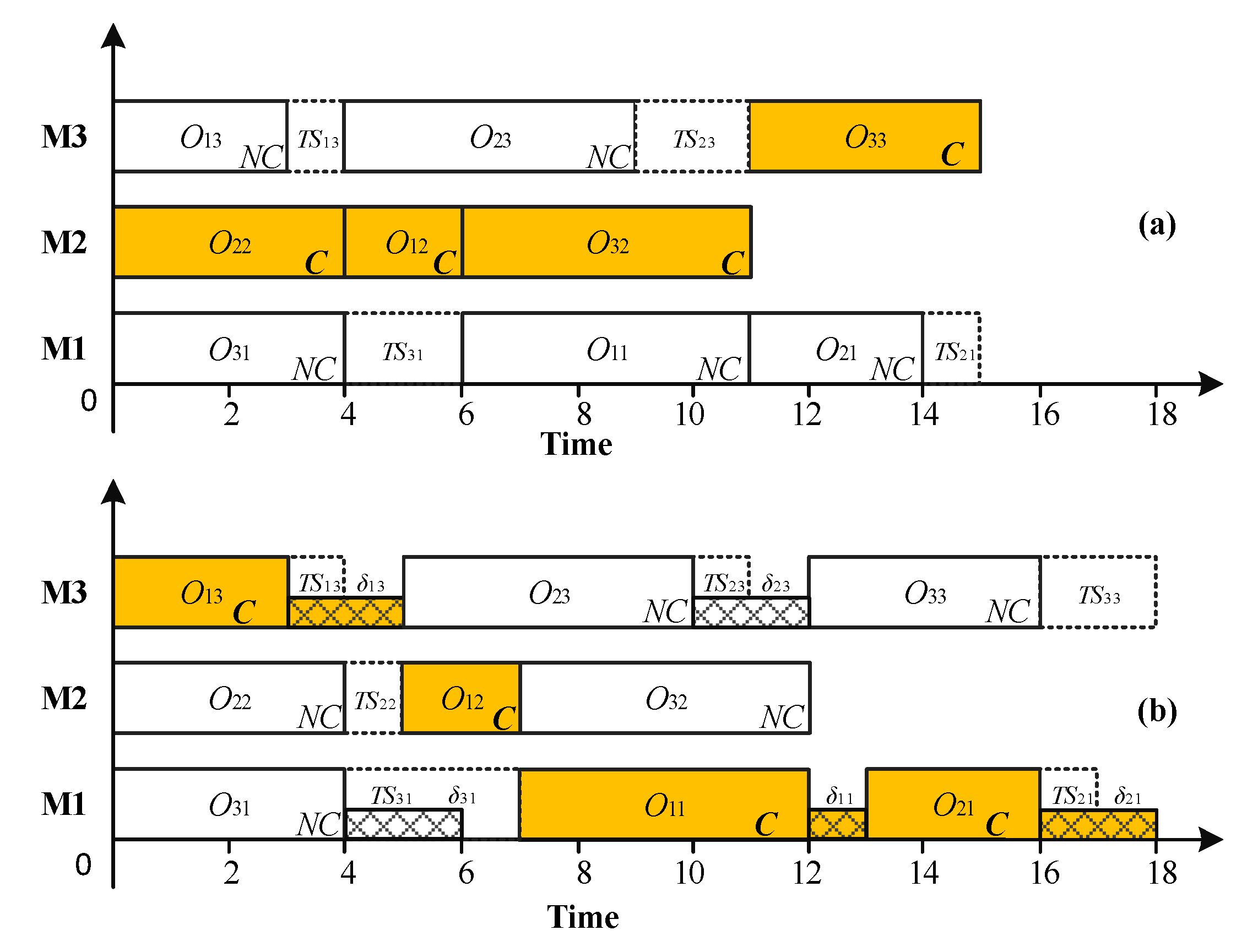
The disturbances on the non-critical path can be partially or totally absorbed due to the existence of total slacks while the disturbances occurred on the critical path would lead to higher robustness degradation since there is no slack time to absorb the disturbance. Therefore, to absorb as much disturbance as possible, the disturbances allocated to the critical path should be less. However, inspired by the surrogate measure proposed by Goren et al. [21], when it comes to design the SMs for SJSSP, it is not reasonable to simply consider the disturbance on the critical path. If non-critical operations are allocated with so much disturbance that cannot be totally absorbed by the slacks, the non-critical operation would possibly become a critical operation and affect the predictive makespan of the schedule. To demonstrate the importance of considering the disturbance on both the critical path and non-critical path, we provide an example with three jobs and three machines supposing partial operations are uncertain. The process information of the operations is listed in

Table 1. An stochastic job shop scheduling problem (SJSSP) instance with three jobs and three machines.

Jobs	The Process Constraints of Each Job $({\mathit{M}}_{\mathit{j}}, {\mathit{\mu }}_{\mathit{i}\mathit{j}}, {\mathit{\sigma }}_{\mathit{i}\mathit{j}}^2)$
	Operation 1	Operation 2	Operation 3
J1	(3, 3, 0.74)	(2, 2, 0)	(1, 5, 0.18)
J2	(2, 4, 0)	(3, 5, 0.74)	(1, 3, 0)
J3	(1, 4, 0)	(2, 5, 0)	(3, 4, 0)

, which are denoted by the vector $(M_j, {\mu }_{ij}, {\sigma }_{ij}^2)$.

One scheduling scenario given in Table 1 is analyzed as shown in Figure 1. The makespan of the schedule is 15 time units, shown in Figure 1a; the critical operations are indicated by bolded C, and non-critical operations are indicated by NC. The possible realized schedule when considering the potential disturbances is shown in Figure 1b. The total slacks that can be used to absorb the disturbances are denoted by $T{S}_{ij}$ (seven time units in total) while the disturbance denoted by ${\delta }_{ij}$ is represented by the upper bound of the stochastic processing time. For example, if we set $\alpha =0.01$, then the maximal disturbance is estimated by ${\delta }_{ij}=2.33{\sigma }_{ij}$. If the predictive schedule is executed, the possible maximal total performance degradation caused by the disturbance will be less than three time units with a probability of 0.99. From Figure 1a, we assume that all of the operations with stochastic processing times are located on the non-critical path while some of the non-critical operations are possibly turned into critical operations. Comparing Figure 1a, and Figure 1b, the critical operations $O_{22}$, $O_{32}$ and $O_{33}$ would possibly turn into non-critical operations due to the processing times of non-critical operations $O_{13}$, $O_{11}$ and $O_{21}$ are increased and turned into critical operations. In this case, assigning all of the operations with disturbances to the non-critical path is unreasonable. In fact, the disturbance should be assigned to both the critical operations and non-critical operations so as to balance the robustness degradation of the non-critical path and the critical path from an overall perspective.

Essentially, the capability of absorbing disturbances of a schedule is determined by the total amount of free slacks. However, the free slacks may be shared by several non-critical operations because they may have the common total slacks. To make full use of the slacks, the total slacks and free slacks are focused on in the following section with the aim of assessing the ability to absorb the disturbance’s effect for the scheduling solutions.

3.2.3. New SMs for Robustness Scheduling

As the previous analysis, minimizing the disturbances on the critical path may allocate more disturbances on the non-critical operations. Therefore, it is important to balance the disturbances assigned to the critical operation set and to the non-critical operation set. Meanwhile, there are two possibilities that determine the maximum robustness degradation when the predictive schedule is executed in the real-world manufacturing environment. The first possibility is that the total disturbances on the critical path determine the robustness degradation. The second possibility is that the disturbances on the non-critical path play a leading role when the disturbances assigned to the critical path are apparently less than those assigned to the non-critical path. Therefore, minimizing the maximum robustness degradation can be conducted by considering two strategies. We first suggest SM4 to estimate and optimize the scheduling robustness based on minimizing the total influence of disturbances on the critical path and non-critical path from an overall perspective. Then, we suggest SM5 minimizing the maximum of the robustness degradation on the critical operation set and on the non-critical operation set. The suggested SMs are represented by Equations (14) and (15):

$$SM4 = S{M}_{\mathrm{cp}}+S{M}_{\mathrm{ncp}}$$

(14)

$$SM5 = \max \{S{M}_{\mathrm{cp}},\hspace{0.17em}\hspace{0.17em}S{M}_{\mathrm{ncp}}\}$$

(15)

where $S{M}_{\mathrm{cp}}$ and $S{M}_{\mathrm{ncp}}$ denote the estimated robustness degradation on the critical path and the non-critical path, respectively. SM4 is based on minimizing the overall possible robustness degradation of the predictive schedule. The reasonability of SM5 is that the non-critical operations would absorb a certain amount of disturbances; meanwhile, the critical operations may transform into non-critical operations and get a certain amount of disturbance absorption capability. Therefore, it will also have the ability to estimate the possible robustness degradation by minimizing the maximum robustness degradation on the critical path and non-critical path.

In SM4 and SM5, the calculation of $S{M}_{\mathrm{cp}}$ should consider all of the critical operations. The reason is that if only the critical path with the largest sum variance is considered, other critical operations would be neglected since the robustness evaluation of the non-critical operation set will not consider the remaining critical operations. Therefore, the total disturbance on the critical operation set should be estimated to consider all of the variance of the critical operations. Given that there is no slack on the critical operations, the maximum possible disturbance on the critical operation set is estimated by:

$$S{M}_{\mathrm{cp}}{= \mathrm{Z}}_{\alpha }\sqrt{{\displaystyle \sum _{h=1}^{N_{\mathrm{cp}}}{\sigma }_h{}^2}},h=1,2,...,N_{\mathrm{cp}}$$

(16)

where $N_{\mathrm{cp}}$ denotes the total number of critical operations and ${\mathrm{Z}}_{\alpha }$ denotes the critical value determined by the predefined confidence level $(1-\alpha )$.

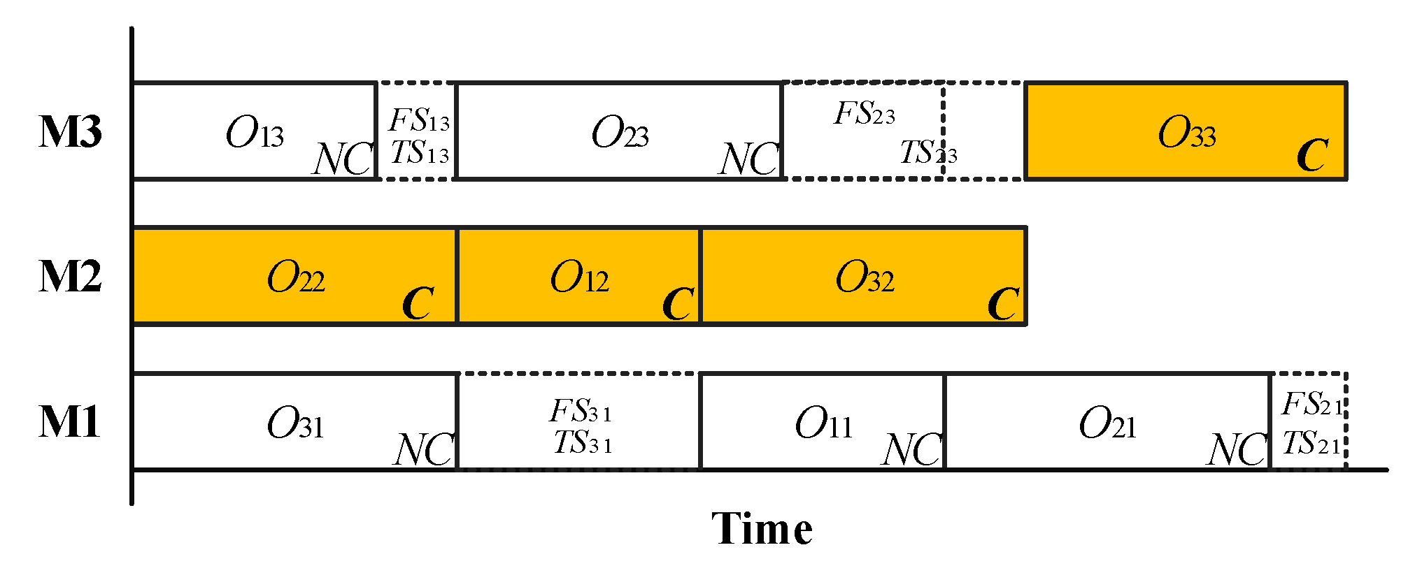
In the non-critical operation sets, the disturbances can be partially or totally absorbed by the total slacks. Then the maximum disruptions can be estimated by using the maximum possible disturbance that is estimated by the right-sided probability distribution function. Therefore, the main problem that should be tackled is how to determine the disturbance absorption capability based on the total slacks and free slacks in the predictive schedule. As shown in Figure 2, a Gantt chart is used to analyze the strategy of assessing the disturbance absorption capability.

In the non-critical operation set, there are five operations that have total slacks to absorb disturbances, namely $O_{13}$, $O_{23}$, $O_{31}$, $O_{11}$, and $O_{21}$. However, the total slacks of some operations are greater than its corresponding free slacks. For example, $F{S}_{23}<T{S}_{23}$ for operation $O_{23}$, so the disturbance in $O_{23}$ will occupy the total slack of the succeeding operation $O_{21}$ if the disturbance cannot be completely absorbed in the case of $F{S}_{23}<{\delta }_{23}$. Besides, $F{S}_{11}$ of operation $O_{11}$ is equal to zero when $T{S}_{11}=T{S}_{21}$, which means $F{S}_{21}$ of operation $O_{21}$ is shared by the operations $O_{11}$, $O_{21}$ and possibly $O_{23}$ if $F{S}_{23}$ cannot absorb the disturbance completely. From the above analysis, the total slacks may be occupied by a single operation or shared by several operations, which leads to directly evaluating the disturbance absorption capability intractable. To estimate the disturbances absorptive capability, an approximate equivalent method is proposed to calculate the occupation rate of total slacks for the operations that share the common total slacks. The basic idea is that the maximum capability of absorbing the disturbances is determined by the total quantity of free slacks. We use the mean ratio to denote the occupation coefficient of each operation since the total slacks are shared by all non-critical operations. The average slack occupation coefficient of each operation for any schedule is estimated by:

$${\epsilon }_0={\displaystyle \sum _{i=1}^n{\displaystyle \sum _{j=1}^{m}F{S}_{ij}}}/{\displaystyle \sum _{i=1}^n{\displaystyle \sum _{j=1}^{m}T{S}_{ij}}}$$

(17)

where ${\epsilon }_0$ denotes the basic average occupation coefficient of total slacks. However, the average occupation coefficient should be modified because the critical operations in the predictive schedule need to be excluded when calculating the average occupation coefficient of non-critical operations. Therefore, the average occupation coefficient should be modified by considering that the critical operations do not share the free slacks. After removing the critical operations, the average occupation coefficient is modified as:

$$\epsilon =\frac{1}{(1-N_{\mathrm{cp}}/mn)}{\epsilon }_0=\frac{mn}{(mn-N_{\mathrm{cp}})}{\epsilon }_0$$

(18)

where $\epsilon$ is adopted to estimate the occupation rate of each operation in a schedule. Then, the disturbance absorption capability $C_k$ for each operation is estimated by:

$$C_k=\frac{mn{\displaystyle \sum _{i=1}^n{\displaystyle \sum _{j=1}^{m}F{S}_{ij}}}}{(mn-N_{\mathrm{cp}}){\displaystyle \sum _{i=1}^n{\displaystyle \sum _{j=1}^{m}T{S}_{ij}}}}T{S}_k, k=1, ...,N_{\mathrm{ncp}}$$

(19)

Therefore, the possible robustness degradation in non-critical operation set is calculated by:

$$S{M}_{\mathrm{ncp}}={\displaystyle \sum _{k=1}^{N_{\mathrm{ncp}}}{\delta }_k},k=1, 2, ..., N_{\mathrm{ncp}}$$

(20)

where ${\delta }_k$ represents the processing time deviation of any non-critical operation in the non-critical operation set with $N_{\mathrm{ncp}}$ elements. Therefore, the maximum possible disturbance of each non-critical operations is estimated by:

$${\delta }_k=\{\begin{array}{cc}\left|C_k-Z_{\alpha }{\sigma }_k\right|, & \mathrm{if} C_k-Z_{\alpha }{\sigma }_k<0\\ 0,& \mathrm{otherwise}\end{array}$$

(21)

After the robustness evaluation function has been formulated, SM4 and SM5 are rewritten as:

$$SM4{=\mathrm{Z}}_{\alpha }\sqrt{{\displaystyle \sum _{h=1}^{N_{\mathrm{cp}}}{\sigma }_h{}^2}}+{\displaystyle \sum _{k=1}^{N_{\mathrm{ncp}}}{\delta }_k}$$

(22)

$$SM5=\max \left\{{\mathrm{Z}}_{\alpha }\sqrt{{\displaystyle \sum _{h=1}^{N_{\mathrm{cp}}}{\sigma }_h{}^2}},\hspace{0.17em}\hspace{0.17em}{\displaystyle \sum _{k=1}^{N_{\mathrm{ncp}}}{\delta }_k}\right\}$$

(23)

where $h=1, ...,N_{\mathrm{cp}}$, $k=1, ..., N_{\mathrm{ncp}}$. By using the above quantified equations, the robustness of the predictive schedule can be effectively estimated. Therefore, the robust predictive schedule can be identified by using the presented SMs.

4. HEDA for SJSSP

4.1. Framework of HEDA

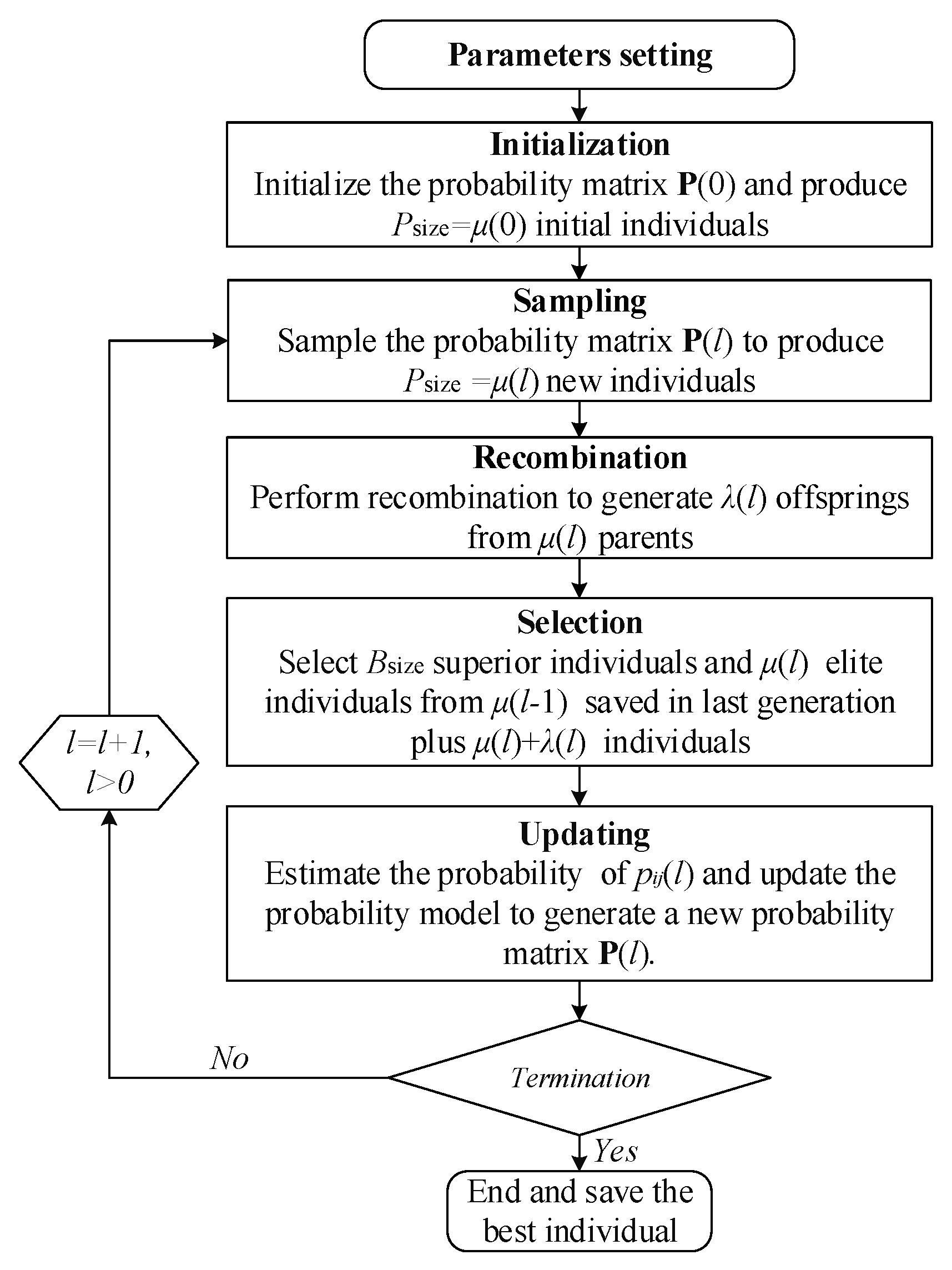
To optimize the SJSSP, the HEDA proposed by Xiao et al. [34] is adopted. To enhance the population diversity of EDA [35], the recombination process and $(\mu +\lambda )$ selection method of $(\mu +\lambda )-\mathrm{ES}$ [36] are combined with EDA. The procedure is shown in Figure 3.

The first step is to set the parameters, and then the probability matrix for sampling the initial individuals is initialized. The recombination method is executed to enhance the population diversity of the EDA. In the selection process, $B_{\mathrm{size}}$ individuals for updating the probability model are selected. Meanwhile, $\mu (l)$ elite individuals are saved for the next iteration. The detailed procedures of the HEDA are presented in the following sections.

4.2. Encoding and Decoding

An operation-based encoding scheme is adopted. Each individual of the population denotes a schedule solution of the SJSSP, which is represented by a sequence of the operations. The operations of the job $J_i$ are represented by $[(i-1)m+1,...,(i-1)m+j,...,(i-1)m+m]$. Let $\pi =[{\pi }_1,...,{\pi }_k,...,{\pi }_{m\times n}]$, where $k=1,...,m\times n$ denotes $m\times n$ positions in each individual. Under this encoding scheme, $(i-1)m+j$ in the position of ${\pi }_k$ in $\pi$ denotes that the $j\mathrm{th}$ operation of the job $J_i$ is located at the $k\mathrm{th}$ position of $\pi$. The individual is encoded under the constraints of process precedence, so it will never produce infeasible solutions in both the population initialization process and the individual sampling process. In addition, the active decoding method used in the study of Wang and Zheng [37] is adopted to decode the schedule solution, in which the set of active schedules is a subset of the semi-active ones and an optimal solution must be an active schedule to the regular index makespan. By converting the semi-active schedule to the active one, the makespan can be shortened. In this study, the decoding process uses the expected processing times when generating the predictive schedule; when conducting the simulation based robustness evaluation, the decoding process will use the simulated processing time scenario.

4.3. Probability Model and Updating Mechanism

In the HEDA, the new individuals in each generation are sampled according to their probability model such that the superior population can be generated from the most promising area in the solution space [38]. A probability matrix $P(l)=\left\{p_{ij,{\pi }_k}^l\right|i=1,2,...n;j=1,2,...,m;k=1,...,m\times n\}$ with $m\times n$ rows and $m\times n$ columns is designed for SJSSP considering the encoding scheme. A more detailed description of $P(l)$ is shown as:

$$P(l)=\left(\begin{array}{cccc}{p}_{11,{\pi }_1}^l& p_{11,{\pi }_2}^l& \cdots & p_{11,{\pi }_{m\times n}}^l\\ p_{12,{\pi }_1}^l& p_{12,{\pi }_2}^l& \dots & p_{12,{\pi }_{m\times n}}^l\\ ⋮& ⋮& ⋮& ⋮\\ p_{1m,{\pi }_1}^l& p_{1m,{\pi }_2}^l& \cdots & p_{1m,{\pi }_{m\times n}}^l\\ p_{21,{\pi }_1}^l& p_{21,{\pi }_2}^l& \dots & p_{21,{\pi }_{m\times n}}^l\\ p_{22,{\pi }_1}^l& p_{22,{\pi }_2}^l& \cdots & p_{22,{\pi }_{m\times n}}^l\\ ⋮& ⋮& ⋮& ⋮\\ p_{2m,{\pi }_1}^l& p_{2m,{\pi }_2}^l& \cdots & p_{2m,{\pi }_{m\times n}}^l\\ ⋮& ⋮& ⋮& ⋮\\ p_{n1,{\pi }_1}^l& p_{n1,{\pi }_2}^l& \cdots & p_{n1,{\pi }_{m\times n}}^l\\ p_{n2,{\pi }_1}^l& p_{n2,{\pi }_2}^l& \cdots & p_{n2,{\pi }_{m\times n}}^l\\ ⋮& ⋮& ⋮& ⋮\\ p_{nm,{\pi }_1}^l& p_{nm,{\pi }_2}^l& \cdots & p_{nm,{\pi }_{m\times n}}^l\end{array}\right)$$

(24)

The element $p_{ij,{\pi }_k}^l$ in the probability matrix $P(l)$ represents the probability of the $j\mathrm{th}$ operation of job $J_i$ located in the position ${\pi }_k$ in a schedule, and $l$ denotes the generation. The probability function of the superior population $B_{\mathrm{size}}$ is written as:

$$p_{ij,{\pi }_k}^l={\displaystyle {\sum }_{s=1}^{B_{\mathrm{size}}}\frac{I_{ij,{\pi }_k}\left(l\right)}{B_{\mathrm{size}}}},\forall i,j,k$$

(25)

where $I_{ij,{\pi }_k}(l)$ defines the statistical function as follows:

$$I_{ij,{\pi }_k}(l)=\{\begin{array}{l}\begin{array}{l}1,\mathrm{if} \mathrm{the} j\mathrm{th}\mathrm{operation} \mathrm{of} \mathrm{job} J_i \mathrm{appears}\\ \mathrm{in} \mathrm{position} {\pi }_k\mathrm{of} \mathrm{a} \mathrm{schedule}\end{array}\hfill \\ 0,\mathrm{otherwise}\hfill \end{array}$$

(26)

To update the probability matrix of each generation, an incremental learning rule in the field of machine learning is adopted. The learning function is presented as:

$$p_{ij,{\pi }_k}^{l+1}=(1-\beta )p_{ij,{\pi }_k}^l+\beta \frac{1}{B\mathrm{size}}{\displaystyle {\sum }_{s=1}^{B_{\mathrm{size}}}[I_{ij,{\pi }_k}(l)]}$$

(27)

where $p_{ij,{\pi }_k}^{l+1}$ denotes the probability of the $j\mathrm{th}$ operation of job $J_i$ located in the position ${\pi }_k$ of the generation $l+1$, and $\beta (0<\beta <1)$ denotes the learning rate.

4.4. Initializing and Sampling

In the phase of population initialization, the entire solution space would be sampled uniformly by $P(0)$ via the roulette wheel selection method. In each generation of the HEDA, the new individuals are generated via sampling the solution space according to the probability matrix $P(l)$. The individual sampling algorithm is shown as follows:

Step 1. Initialize the candidate operation matrix $Q_{m\times n}=\{O_{ij}:i=1,2,...,n,j=1,\mathrm{2....},m\}$, which is used to store the operations sequenced by considering the process constraints;

Step 2. While $k<m\times n$ do

Step 2.1. Select the optional operation vector $Q_{m\times 1}^{\mathrm{opt}}$, $Q_{m\times 1}^{\mathrm{opt}}(k)\subseteq Q_{m\times n}, k=1,...,m\times n$ by selecting only the immediate succeeding operations those needed to be processed following the process constraints;

Step 2.2. Obtain the probability of each operation in the operation set $Q_{m\times 1}^{\mathrm{opt}}(k)$, which is possibly located in the position${\pi }_k$according to the probability matrix $P(l)$;

Step 2.3. Normalize the probability of each operation that belongs to operation set $Q_{m\times 1}^{\mathrm{opt}}(k)$ by equation $p{\prime }_{ij,{\pi }_k}=p_{ij,{\pi }_k}/{\displaystyle \sum p_{ij,{\pi }_k}}$, for all $O_{ij}\in Q_{m\times 1}^{\mathrm{opt}}(k)$, and then, select an operation by the roulette algorithm according to the normalized probability, then put the selected operation in the location ${\pi }_k$ of $\pi =[{\pi }_1,...,{\pi }_k,...,{\pi }_{m\times n}]$;

Step 2.4 Delete the selected operation in candidate operation set $Q_{m\times n}$;

End While

Step 3. Return the newly generated individual S.

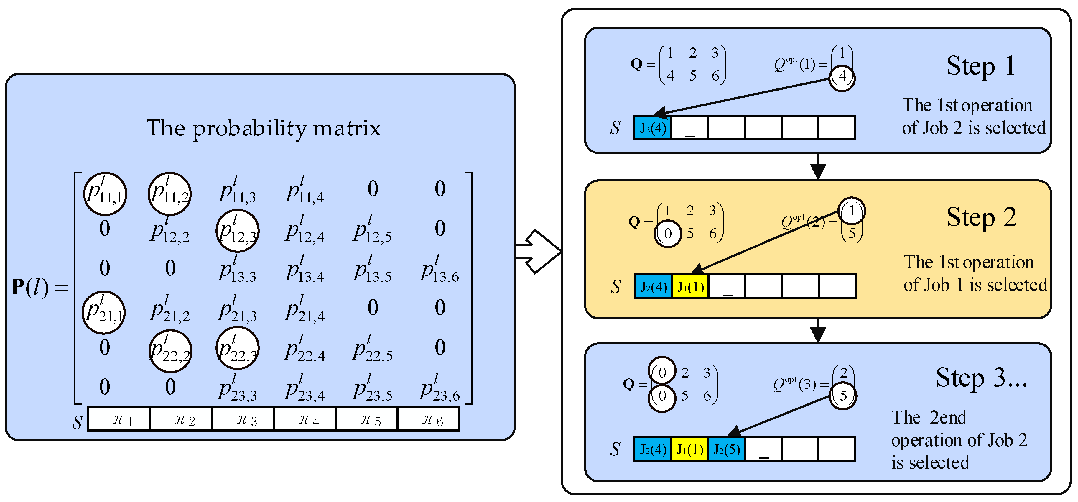
To describe the sampling algorithm more detailed, we use a problem instance with two jobs and three machines to illustrate the statistical probability of each operation. By the encoding scheme, the three operations of job $J_1$ are denoted by [1, 2, 3]; the three operations of job $J_2$ are denoted by [4, 5, 6]. By using Equation (24), the probability matrix of the problem instance is shown as Equation (28):

$$P(l)=\left[\begin{array}{cccccc}{p}_{11,1}^l& p_{11,2}^l& p_{11,3}^l& p_{11,4}^l& p_{11,5}^l& p_{11,6}^l\\ p_{12,1}^l& p_{12,2}^l& p_{12,3}^l& p_{12,4}^l& p_{12,5}^l& p_{12,6}^l\\ p_{13,1}^l& p_{13,2}^l& p_{13,3}^l& p_{13,4}^l& p_{13,5}^l& p_{13,6}^l\\ p_{21,1}^l& p_{21,2}^l& p_{21,3}^l& p_{21,4}^l& p_{21,5}^l& p_{21,6}^l\\ p_{22,1}^l& p_{22,2}^l& p_{22,3}^l& p_{22,4}^l& p_{22,5}^l& p_{22,6}^l\\ p_{23,1}^l& p_{23,2}^l& p_{23,3}^l& p_{23,4}^l& p_{23,5}^l& p_{23,6}^l\end{array}\right]=\left[\begin{array}{cccccc}{p}_{11,1}^l& p_{11,2}^l& p_{11,3}^l& p_{11,4}^l& 0& 0\\ 0& p_{12,2}^l& p_{12,3}^l& p_{12,4}^l& p_{12,5}^l& 0\\ 0& 0& p_{13,3}^l& p_{13,4}^l& p_{13,5}^l& p_{13,6}^l\\ p_{21,1}^l& p_{21,2}^l& p_{21,3}^l& p_{21,4}^l& 0& 0\\ 0& p_{22,2}^l& p_{22,3}^l& p_{22,4}^l& p_{22,5}^l& 0\\ 0& 0& p_{23,3}^l& p_{23,4}^l& p_{23,5}^l& p_{23,6}^l\end{array}\right]$$

(28)

in which the statistical probability of the operations that violate the process constraints is zero. After the operation has been selected and placed on the corresponds position, the probability of the remained optional operations needs to be normalized, then the new optional operation can be selected by the normalized probability. For example, if the first operation of Job 2 is first selected, then the first operation of Job 1 is selected, in sequence, the sampling process by using the above probability matrix can be described by Figure 4.

In Figure 4, the operations in the individual are selected according to the statistical probability. The procedure will be continued following the above sampling algorithm until the candidate operation set becomes empty. In this sampling method, the process constraints are under consideration, so there exists no infeasible individual.

4.5. Recombination and Selection

To enhance population diversity and avoid premature convergence in the evolutionary process of the EDA, a recombination method based on the inherit ratio of parent operation is used [34].

After decoding and evaluating the individuals by using the objective function, the promising individuals will be selected and saved. In the $(\mu +\lambda )$ selection process, a deterministic sorting method of evolutionary strategy is adopted. Specifically, in each generation, $\mu$ new individuals will be generated, and $\lambda$ offspring will be obtained by recombining the $\mu$ parent individuals saved in the last generation. In the selection block of the HEDA, the performance values of $N_{\mathrm{good}}$ individuals obtained by $\mu$ elite individuals in the last generation are sorted in ascending order, then the $B_{\mathrm{size}}$ superior population and $\mu$ elite individuals are saved to update the probability model for the next generation.

5. Computational Experiments

5.1. Experiment Settings

The experimental analysis approach and the HEDA are both coded by Matlab 2015b (The MathWorks, Inc., Natick, MA, USA) on a computer of Intel(R) Xeon(R) CPU E31230 @ 3.2 GHz with RAM 8.00 GB. In this study, we focus on the performance comparison of different surrogate measures of robustness. For comparability and ease of implementation reasons, all the replications of HEDA are closely related and the parameters are set to the same values.

We first set the parameters according to the experimental purpose and then conduct the simulations under the same computational environment for the purpose of a fair comparison. To improve the computational efficiency of the simulations while keeping the satisfactory performance of the HEDA, the population size ($P_{\mathrm{size}}$) and the evolutionary generation ($gen$) are both set to 100 according to a one-way ANOVA (analysis of variance), in which the experimental results demonstrate that both the evolutionary generation and the population size have no significant performance decreasing under the confidence level of 0.95 (set $\alpha =0.05$). In the next step, we use the Taguchi method of design of experiment (DOE) [39] to select a group of the key parameters of HEDA by using the benchmark FT10 [40], in which the makespan is used as the optimization objective. The value of recombination probability ($R\mathrm{p}$), the learning rate ($\beta$) and the number of the superior population ($B_{\mathrm{size}}$) are tested under four factor levels. For each parameter combination, the HEDA runs 20 times and the average of makespan is obtained. Finally, a group of good parameter combination is selected: $R\mathrm{p}$ = 0.8; $\beta$ = 0.3; $B_{\mathrm{size}}$ = 40. For the details of the experimental results of the ANOVA and the DOE, please refer to the supplementary material.

The number of simulation replications is set to $L=200$, which is enough to approximate the expected value as stated by Ahmadizar et al. [24]. The number of parents individuals (μ) is the same as the population size, by which λ = 100 new offspring will be generated through the recombination process. In addition, the number of positioning jobs is set to $\lfloor n/2\rfloor$ by referring to the previous research [34]. Therefore, the parameters setting of HEDA is shown in

Table 2. The parameters setting of HEDA.

Parameters	Values	Parameters	Values
Population size ($P_{\mathrm{size}}$)	100	Learning rate ($\beta$)	0.3
Evolutionary generations ($gen$)	100	Superior population ($B_{\mathrm{size}}$)	40
Recombination probability ($R\mathrm{p}$)	0.8	Value of μ and λ	100
Number of positioning jobs	$\lfloor n/2\rfloor$	Simulation replications $(L)$	200

.

Since there are no standard benchmark problems for SJSSP, we use the deterministic problem instances and modify them into stochastic versions by introducing variances into the processing times. The benchmarks of FT06, FT10 and FT20 provided by Muth and Thompson [40] and LA06, LA16, LA21, LA26 and LA32 provided by Lawrence [41] are selected. The expected processing times are using the deterministic processing times in the benchmarks. The variances of the processing times are set randomly and the modified benchmarks can be obtained from the authors.

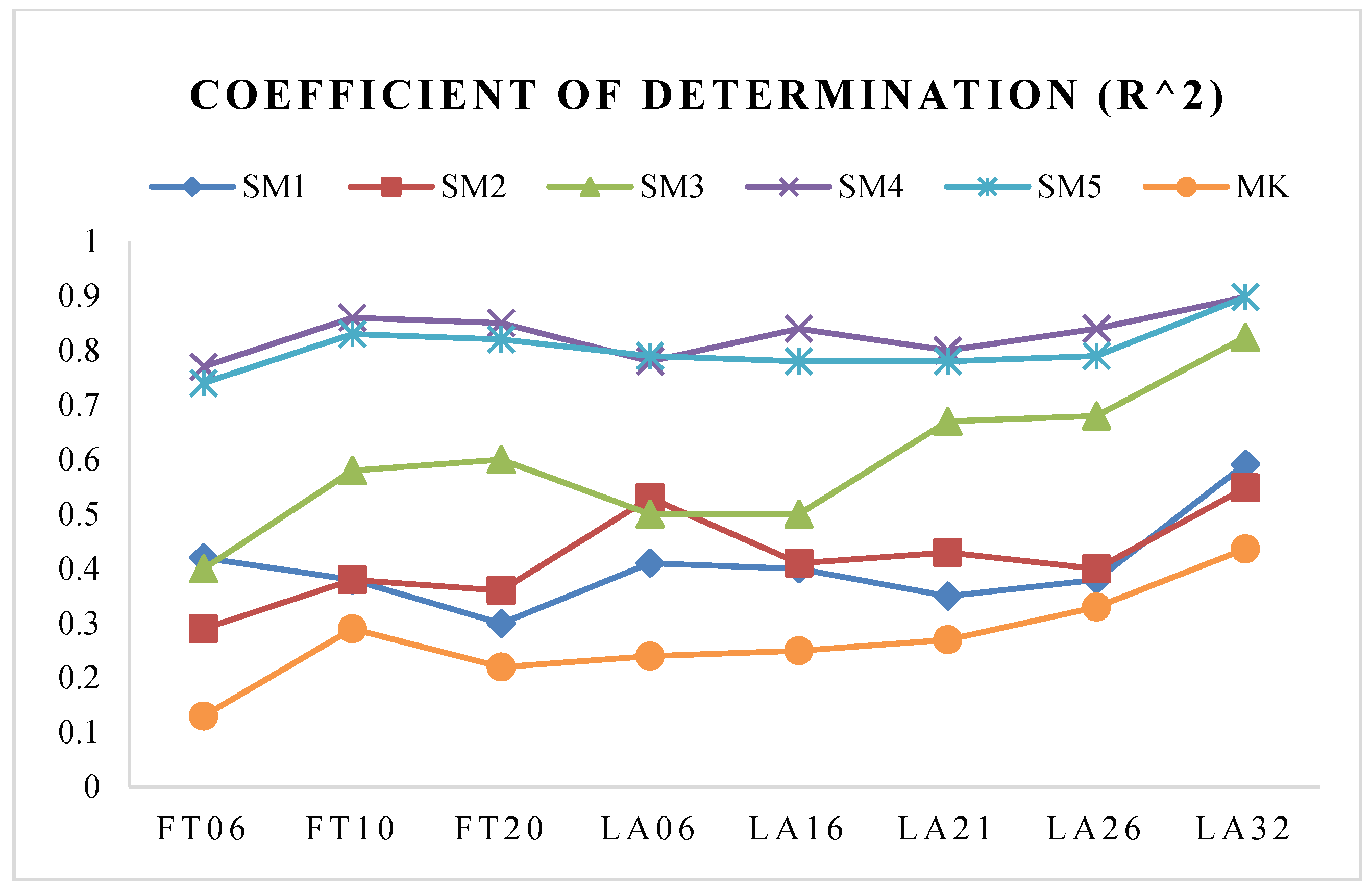
The aim of the first experiment is to investigate the correlation between the SMs and the corresponding simulation-based robustness denoted by SMsim when optimizing the robustness of SJSSP by using the SMs. The coefficient of determination (R² value) of three existing SMs (SM1, SM2, and SM3) and two presented SMs (SM4, SM5) are investigated. The second experiment includes two parts: the first part using a one-way ANOVA to analyze whether the specified confidence level $(1-\alpha )$ has a significant effect on the performance of the proposed SMs. The second part is to verify the effectiveness of SMs and the computational efficiency.

To compare the performances of SMs under different degrees of uncertainty, five ULs are considered. For example, the UL with 20% uncertain operations is denoted by UL2. The uncertain operations are randomly selected by a uniformly distributed number $x_{ij},x_{ij}\in \mathrm{U} [0,1]$with the following steps:

Step 1. For each operation $O_{ij}$, generate a number $x_{ij}$ randomly;

Step 2. If $x_{ij}<UL,UL=0.2,0.4,...,1$, the processing time of operation $O_{ij}$ is allocated with a prespecified variance ${\sigma }_{ij}^2$ and transformed into an uncertain operation; the variance is set at ${\sigma }_{ij}^2=0$, otherwise.

5.2. Correlation Analysis of the SMs

To evaluate the correlation between SMs and the corresponding simulation-based robustness (SMsim), we analyze the coefficient of determination (R² value). The weight coefficient of robustness measure is set as $\eta = 1$ then the robustness can be analyzed independently without being affected by the makespan (MK). The values of SMsim can also be calculated by Equation (1).

The R² values are obtained from the regression of the values of SMs and the corresponding SMsim in the optimization process of HEDA with 100 generations. The higher the R² values between the SMs and SMsim, the better the performance to estimate and optimize the robustness. In the simulation, the critical value is set as $Z_{\alpha }= 1.96$ with a confidence level of 0.975. The algorithm for correlation analysis is shown as follows:

Step 1. Select the best schedule in each generation, and save the values of SMs of each schedule in each run of HEDA;

Step 2. Use Monte Carlo simulation to calculate the value of SMsim for the selected schedule:

Step 2.1. Generate the processing time scenario using the known probability distribution;

Step 2.2. Decode the schedule using the randomly-generated processing time scenario and then obtain and save the possible realized makespan $\xi C_{\max }^l,l=1,2,...,L$ of each simulation replication;

Step 2.3. Repeat Step 2.2 for $L$ times, and calculate the SMsim value by Equation (1);

Step 3. Calculate the R² value between SMs and its corresponding SMsim.

The analyzed R² value in the following is represented by the average value of 20 runs of HEDA. As the comparison measures, SM1, SM2 and SM3 are investigated. The measure MK is also examined, which is conducted by only optimizing the makespan (set $\eta = 0$) to analyze the correlation between optimizing the makespan and its corresponding simulation-based robustness under different ULs.

Table 3. The R² values for the regression between SMs and SMsim. UL: uncertainty level; MK: makespan.

Benchmarks	Measures	Uncertainty Levels
		UL2	UL4	UL6	UL8	UL10	Average
FT06 Size: 6 × 6	SM1	0.44	0.46	0.29	0.55	0.53	0.45
	SM2	0.27	0.09	0.14	0.48	0.53	0.30
	SM3	0.15	0.13	0.26	0.23	0.14	0.18
	SM4	0.69	0.72	0.83	0.69	0.87	0.76
	SM5	0.71	0.77	0.74	0.73	0.76	0.74
	MK	0.15	0.17	0.14	0.10	0.14	0.14
FT10 Size: 10 × 10	SM1	0.13	0.19	0.39	0.69	0.77	0.43
	SM2	0.14	0.16	0.44	0.56	0.72	0.40
	SM3	0.53	0.57	0.59	0.48	0.70	0.57
	SM4	0.82	0.90	0.89	0.89	0.85	0.87
	SM5	0.78	0.83	0.83	0.86	0.85	0.83
	MK	0.09	0.27	0.26	0.27	0.73	0.32
FT20 Size: 20 × 10	SM1	0.03	0.12	0.35	0.48	0.76	0.35
	SM2	0.14	0.31	0.35	0.40	0.73	0.39
	SM3	0.44	0.67	0.62	0.59	0.68	0.60
	SM4	0.84	0.83	0.90	0.84	0.81	0.84
	SM5	0.84	0.76	0.87	0.79	0.82	0.82
	MK	0.11	0.06	0.18	0.30	0.67	0.26
LA06 Size: 15 × 5	SM1	0.53	0.61	0.31	0.18	0.58	0.44
	SM2	0.46	0.49	0.45	0.68	0.87	0.59
	SM3	0.51	0.56	0.29	0.52	0.40	0.46
	SM4	0.84	0.78	0.67	0.79	0.68	0.75
	SM5	0.87	0.81	0.84	0.73	0.69	0.79
	MK	0.31	0.29	0.08	0.37	0.41	0.29
LA16 Size: 10 × 10	SM1	0.11	0.29	0.46	0.45	0.81	0.42
	SM2	0.20	0.39	0.44	0.55	0.79	0.47
	SM3	0.20	0.20	0.26	0.47	0.77	0.38
	SM4	0.90	0.92	0.83	0.87	0.79	0.86
	SM5	0.81	0.75	0.73	0.81	0.80	0.78
	MK	0.06	0.16	0.28	0.31	0.71	0.30
LA21 Size: 15 × 10	SM1	0.20	0.20	0.26	0.47	0.77	0.38
	SM2	0.24	0.22	0.45	0.47	0.84	0.44
	SM3	0.55	0.59	0.57	0.71	0.68	0.62
	SM4	0.79	0.80	0.82	0.78	0.80	0.80
	SM5	0.84	0.78	0.71	0.78	0.80	0.78
	MK	0.06	0.10	0.23	0.42	0.67	0.30
LA26 Size: 20 × 10	SM1	0.10	0.15	0.37	0.64	0.71	0.39
	SM2	0.16	0.39	0.50	0.58	0.78	0.48
	SM3	0.64	0.70	0.74	0.65	0.71	0.69
	SM4	0.83	0.85	0.82	0.87	0.77	0.83
	SM5	0.81	0.83	0.80	0.84	0.82	0.82
	MK	0.08	0.12	0.41	0.56	0.70	0.37
LA32 Size: 30 × 10	SM1	0.42	0.37	0.54	0.77	0.86	0.59
	SM2	0.40	0.35	0.41	0.70	0.89	0.55
	SM3	0.67	0.83	0.88	0.87	0.87	0.82
	SM4	0.88	0.94	0.92	0.88	0.87	0.90
	SM5	0.85	0.91	0.92	0.92	0.90	0.90
	MK	0.29	0.34	0.39	0.46	0.69	0.44

shows the simulation results.

In Table 3, the average R² values under five ULs for the benchmarks are provided. The resultant average R² values of the suggested SM4, SM5 are apparently higher than those obtained by SM1, SM2 and SM3, in which the lowest value is 0.67 in LA06 under UL6. Further analysis finds that slightly lower average R² values of the suggested SMs exist in the benchmarks with a small size under lower or medium ULs, such as the cases in FT06 and LA06. The reason lies in that the disturbances are easily absorbed and then the optimization process of small-sized benchmarks under lower ULs are much easier to converge to the optimum within several generations.

The suggested SM4, SM5 are highly correlated with the robustness measure under all of the ULs. However, the variation of the R² values of SM1, SM2, SM3 and MK is quite obvious. For SM1, the average R² value is increasing gradually from UL2 to UL10, which is as high as 0.81 under UL10 of LA16, but, the average R² value is very low under lower ULs. Part of the reason lies in that SM1 only considers the average total slack while the available information is neglected. The average R² values of SM2 and SM3 show the similar characteristic as SM1, that is the higher the ULs, the higher the correlations. Therefore, the SM1, SM2, and SM3 are not well applicable to the SJSSP under all of the ULs, even if they show slightly higher correlation under higher ULs. Concerning the average R² values of MK, it is also found that the correlation is increased with the increasing of UL. The main reason is that the optimization of MK would decrease the length of the critical path, as well as the total number of operations on the longest critical path at the higher ULs, which has the potential to decrease the total disturbances on the critical path.

To further compare the average R² values of the suggested SMs and the existing SMs, the average R² values under five ULs on all of the benchmarks are shown in Figure 5. It is found that the average R² values of the suggested SM4, SM5 are apparently greater than those of SM1, SM2 and SM3 over all of the benchmarks. Among the three existing SMs, SM3 shows the highest correlation, which means that minimizing the maximum sum of variance on the critical path is better than considering only the average total slacks or the number of potential critical operations. From the above analyses, it is concluded that the correlation values of the suggested SM4, SM5 are apparently higher than those of the existing SMs, so the suggested SMs can estimate the robustness of the schedule more accurately. The performance of the optimal robustness needs to be evaluated further. However, the performance analyses of SM1, SM2 and SM3 are not conducted, since the average R² values are apparently lower.

5.3. The Performance of the SMs

5.3.1. One-Way ANOVA Analysis for Different Confidence Levels

To further investigate the effect of the different predefined confidence levels of the processing time’s disturbance on the performance of the proposed SMs, a one-way ANOVA test on the average R² values of the presented SMs is performed by using the modified benchmarks of FT06, FT10 and FT20. The UL10 is selected because the trial would be more reliable under the most severe UL, which means all of the operations are uncertain. We first conduct the normality test of the data before the implement the ANOVA. The effects are considered significant if the p-value is less than 0.05.

In this experiment, three confidence levels for setting the maximum disturbances of stochastic processing times, i.e., 0.95, 0.975 and 0.99 are tested. Therefore, the corresponding critical values can be obtained by finding the table of right-sided normal distribution, which are $Z_{\alpha }=1.65$, 1.96 and 2.33, respectively. The null hypothesis is that different $Z_{\alpha }$ values have no significant effect on the mean values of the R² values. If the calculated p-value is greater than the prespecified significant level 0.05, we accept the null hypothesis and conclude that the tested factors have no significant effects on the average R² values.

Table 4. One-way ANOVA results concerning three confidence levels.

Factor	FT06
	SM4		SM5
	F-Ratio	p-Value	F-Ratio	p-Value
$Z_{\alpha }$ value	2.34	0.12	2.38	0.11
	FT10
	SM4		SM5
	F-Ratio	p-Value	F-Ratio	p-Value
$Z_{\alpha }$ value	0.56	0.57	0.71	0.49
	FT20
	SM4		SM5
	F-Ratio	p-Value	F-Ratio	p-Value
$Z_{\alpha }$ value	1.59	0.22	1.72	0.19

shows the F-ratio and the p-value of the one-way ANOVA results for SM4, SM5.

Seen from Table 4, the lowest p-value is equal to 0.11, which is still greater than 0.05; therefore, we conclude that the predefined confidence level of processing time’s disturbance has no significant effect on the performance of SMs at the significance level of 0.05. Hence, the presented SMs provide more choices to the decision makers when different risk averse levels are required.

5.3.2. The Performance Analysis of the SMs

In this section, the performance of the suggested SMs for the robustness optimization is analyzed. As the comparison experiments, the simulation-based robustness values obtained by optimizing the makespan and RMsim are adopted. Optimizing makespan would obtain the schedule with the best makespan without considering robustness, while optimizing the RMsim would get the best robustness without taking the makespan into consideration. The weight $\eta$ in the Equation (3) is set to zero when MK is optimized; $\eta$ is set to one when SMs or RMsim is optimized.

The critical value of the disturbances is set as $Z_{\alpha }=1.96$ with the confidence level of 0.975. The optimization of the measure MK is used to demonstrate the effectiveness of the SMs by comparing the robustness values between using and not using the SMs. The robustness values obtained by SM4, SM5, as well as MK would be transformed into SMsim by using Equation (1), in which the robustness obtained by directly optimizing MK is denoted by RMmk. The average and the standard deviation (Std.) of robustness as well as the associated predictive makespan (with 20 simulation replications) that obtained by optimizing SM4, SM5, RMsim and MK are reported in

Table 5. The average and standard deviation (Std.) of robustness for the comparison measures.

Benchmarks	UL	The Comparison Measures
		SM4		SM5		RMsim		RMmk
		Average	Std.	Average	Std.	Average	Std.	Average	Std.
FT06 Size: 6 × 6	UL2	0.06	0.02	0.90	0.77	0.30	0.73	5.64	0.64
	UL4	0.21	0.37	3.66	0.74	0.35	1.59	7.49	0.35
	UL6	7.37	1.08	5.01	0.52	2.18	0.64	12.06	0.47
	UL8	8.55	1.02	11.61	0.47	8.63	0.96	15.24	0.49
	UL10	15.06	0.95	14.57	0.53	13.15	0.62	17.52	0.26
FT10 Size: 10 × 10	UL2	0.00	0.00	0.00	0.00	0.00	0.00	18.40	6.23
	UL4	6.50	3.11	7.80	7.42	1.50	2.83	46.68	9.73
	UL6	31.24	8.16	28.51	3.84	17.60	2.45	81.26	8.41
	UL8	66.54	5.72	57.13	7.22	54.06	5.82	88.32	5.05
	UL10	103.23	5.84	98.89	4.37	93.14	4.81	108.61	4.95
FT20 Size: 20 × 5	UL2	0.00	0.00	0.00	0.01	0.01	0.03	45.03	5.91
	UL4	0.64	1.18	0.41	0.78	0.00	0.01	79.68	7.68
	UL6	43.46	7.04	24.65	7.62	14.80	2.64	80.19	6.44
	UL8	83.93	6.12	66.37	6.96	51.84	8.04	121.03	4.33
	UL10	126.85	4.31	126.02	2.75	119.65	4.11	132.93	3.90
LA06 Size: 15 × 5	UL2	0.00	0.00	0.00	0.00	0.00	0.00	21.98	0.74
	UL4	0.20	0.66	0.20	0.53	0.00	0.00	27.12	1.62
	UL6	8.52	3.06	4.16	3.18	3.45	1.29	33.69	1.67
	UL8	31.18	2.60	21.78	5.84	14.14	1.53	40.56	2.79
	UL10	45.52	2.37	47.23	3.99	43.60	1.84	60.32	2.87
LA16 Size: 10 × 10	UL2	0.01	0.03	0.08	0.24	0.01	3.27	26.05	0.01
	UL4	5.38	2.53	5.15	0.47	5.25	6.13	24.79	1.69
	UL6	17.73	2.12	20.22	6.28	8.90	4.27	37.59	2.79
	UL8	35.07	3.28	37.78	3.96	30.68	4.17	51.36	1.52
	UL10	64.63	2.09	61.87	1.88	60.90	2.96	68.72	1.79
LA21 Size: 15 × 10	UL2	0.01	0.04	0.01	0.02	0.00	0.00	32.04	5.95
	UL4	2.88	2.67	1.32	2.59	1.69	1.61	31.87	5.91
	UL6	19.55	5.06	21.73	5.31	16.30	1.81	49.93	5.28
	UL8	53.97	5.38	48.16	6.78	46.89	4.80	74.43	6.30
	UL10	87.30	3.94	84.01	4.98	77.43	3.63	90.91	3.12
LA26 Size: 20 × 10	UL2	0.01	0.02	0.00	0.00	0.00	0.00	21.74	5.41
	UL4	4.16	2.43	4.88	4.10	1.06	1.35	39.72	4.85
	UL6	32.79	4.69	28.30	7.52	21.00	3.96	64.40	6.76
	UL8	55.19	7.59	54.45	6.75	54.94	6.08	76.40	7.01
	UL10	90.84	4.54	91.55	6.33	86.54	2.59	99.17	5.72
LA32 Size: 30 × 10	UL2	0.01	0.02	0.09	0.36	0.00	0.01	30.06	10.58
	UL4	24.04	4.12	21.79	6.76	16.32	3.46	58.65	8.85
	UL6	41.91	4.95	34.77	5.97	32.15	6.69	77.71	12.18
	UL8	92.83	7.36	89.33	9.83	87.96	8.98	111.93	10.89
	UL10	134.16	4.74	130.21	7.59	120.98	5.63	144.34	8.99

and

Table 6. The average and Std. of the makespan for the comparison measures.

Benchmarks	UL	The Comparison Measures
		SM4		SM5		RMsim		MK
		Average	Std.	Average	Std.	Average	Std.	Average	Std.
FT06 Size: 6 × 6	UL2	89.5	7.9	80.1	5.3	96.0	11.6	55.0	0.0
	UL4	95.4	12.3	78.1	7.8	75.1	5.7	55.0	0.0
	UL6	78.5	7.9	77.6	4.7	84.8	8.6	55.0	0.0
	UL8	72.1	3.9	70.6	5.6	69.6	2.2	55.0	0.0
	UL10	71.3	4.2	65.7	1.9	64.7	2.7	55.0	0.0
FT10 Size: 10 × 10	UL2	1853.9	142.3	1949.2	170.2	2084.9	110.2	1008.8	17.9
	UL4	1644.3	142.9	1799.2	147.2	1859.0	88.9	1015.7	26.6
	UL6	1523.7	72.5	1477.6	47.5	1674.2	77.4	1019.9	26.4
	UL8	1429.6	49.5	1457.5	68.1	1410.9	77.3	1003.3	32.0
	UL10	1315.1	60.0	1177.8	34.0	1167.6	50.4	1028.4	44.2
FT20 Size: 20 × 5	UL2	2095.5	160.1	2009.8	130.5	2098.9	201.2	1266.9	26.1
	UL4	1800.3	108.3	1953.7	77.4	1990.9	129.9	1257.8	23.5
	UL6	1802.1	89.9	1590.1	38.6	1628.2	58.7	1247.5	25.6
	UL8	1635.9	50.8	1552.5	47.4	1623.4	41.8	1272.9	23.0
	UL10	1461.9	29.1	1383.3	20.8	1418.7	36.2	1251.7	16.5
LA06 Size: 10 × 5	UL2	1451.9	168.1	1543.4	101.7	1608.3	156.6	926.0	0.0
	UL4	1388.9	90.3	1285.0	78.5	1365.6	103.0	926.0	0.0
	UL6	1131.9	67.3	1214.0	76.1	1183.0	55.5	926.0	0.0
	UL8	1070.9	57.2	1156.3	76.1	1083.6	51.0	926.0	0.0
	UL10	1017.4	33.8	991.1	37.5	989.4	13.8	926.0	0.0
LA16 Size: 10 × 10	UL2	1703.7	138.3	1653.9	144.3	1674.1	8.0	998.0	150.4
	UL4	1533.9	117.1	1498.8	76.7	1494.5	16.1	978.0	68.9
	UL6	1347.5	98.5	1318.9	69.1	1377.6	20.5	1014.0	96.8
	UL8	1209.7	54.1	1208.0	47.3	1245.4	16.3	1001.0	98.0
	UL10	1157.2	38.2	1094.9	35.1	1055.3	17.5	987.0	36.3
LA21 Size: 15 × 10	UL2	2149.2	159.0	2322.1	186.1	2232.3	145.5	1188.0	26.0
	UL4	1908.6	132.1	1933.0	118.6	1976.7	130.6	1168.0	28.9
	UL6	1788.0	119.1	1646.9	96.8	1824.0	71.5	1180.0	28.9
	UL8	1547.6	82.6	1610.1	71.6	1529.5	79.9	1230.0	27.5
	UL10	1425.2	65.9	1426.7	70.3	1367.5	44.0	1126.0	29.3
LA26 Size: 20 × 10	UL2	2584.8	280.9	2497.9	152.6	2651.4	203.3	1412.1	48.8
	UL4	2328.3	207.1	2315.6	179.5	2373.7	171.7	1415.3	33.8
	UL6	2168.6	108.9	2178.7	124.5	2119.6	98.2	1398.1	35.7
	UL8	1995.5	64.9	1929.7	62.7	1951.1	131.3	1404.3	29.6
	UL10	1804.4	70.9	1765.2	87.6	1658.8	66.6	1423.7	38.2
LA32 Size: 30 × 10	UL2	3528.4	219.2	3546.9	266.7	3664.8	264.2	2166.4	60.6
	UL4	3310.9	259.8	3174.6	184.2	3282	189.3	2158.3	59.0
	UL6	3136.6	185.6	3027.8	154.8	3090	164.6	2159.7	54.6
	UL8	2897.4	166.7	2913.8	130.9	2774	140.6	2139.4	41.4
	UL10	2708	117.07	2560.5	108.7	2467	121.2	2128.8	51.8

, respectively. Since we mainly focus on the effectiveness of SMs for robustness estimation, the data of the makespan are obtained by decoding the schedule solution using the expected processing times, which is used to show the trend of the makespan when optimizing the robustness by using SMs.

Seen from Table 5, the average of robustness and Std. are almost equal to zero under the lower ULs for all of the benchmarks. The reason is that all of the disruptions can be easily absorbed by assigning the slacks to possible uncertain operations appropriately. Moreover, by comparing the performance between SMs and RMsim, it is evident that the performance of SMs is nearly the same as RMsim under the lower ULs. Meanwhile, the SMs can still improve the robustness of SJSSP efficiently even under the highest UL. As for the Std., the values obtained under different ULs have no noticeable trend except that the Std. of SMs and RMsim are smaller than that obtained by optimizing MK under the lower UL. The variation of the standard deviation is caused by either the randomly-generated uncertain operations in each run of HEDA or by the different optimal solutions of HEDA.

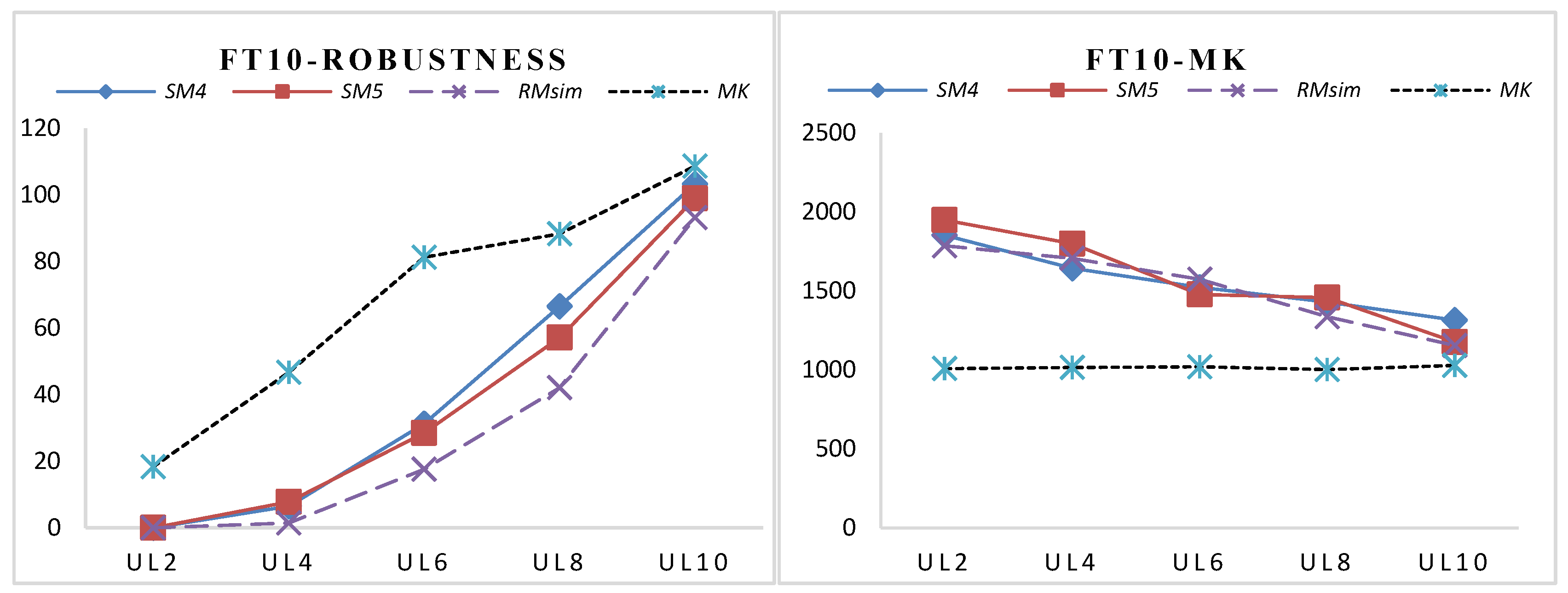
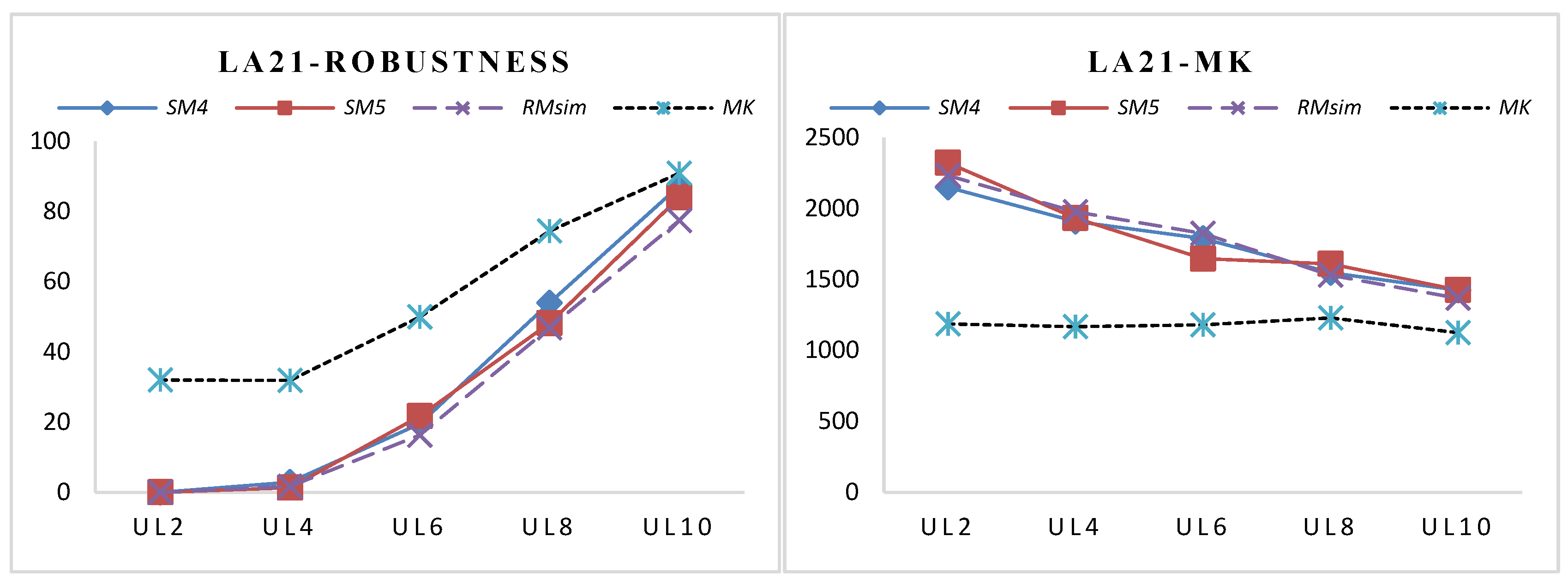
The associated makespan obtained by optimizing the robustness measure would certainly be worse than the makespan by optimizing makespan directly, which can be clearly found in Table 6. However, after the effectiveness of SMs for robustness estimation has been verified, the robust predictive schedule with satisfactory makespan can be easily obtained by optimizing the SMs and the predictive makespan simultaneously with a tremendously lower computational burden. Seen from Table 6, we also find that the average makespan has the trend of decreasing with the increasing of the UL. To show the trend of the SMsim and the associated makespan when the ULs increases, the average of the SMsim and the makespan of two typical benchmarks (FT10 and LA21) are selected and shown in Figure 6 and Figure 7, as the results of other benchmarks show a similar trend.

From Figure 6 and Figure 7, the robustness obtained by only optimizing makespan shows the worst performance, while the robustness obtained by RMsim shows the best in all comparison measures. For all of the benchmarks, the robustness value is increased with the higher ULs. The increasing of the robustness value lies in that the higher the UL, the more serious the disruptions caused by the uncertainties. The performance of each SM will be further analyzed later. Before the analysis, the trend of MK will be discussed.

Seen from the right-side of Figure 6 and Figure 7, we found that as the UL increases, the average makespan values of SMs and RMsim have decreased. The reason lies in that more uncertain operations lead to the increase of the total potential disturbances in the schedule. Consequently, the disturbances on the critical path would also be increased. The robustness degradation on the critical path will decrease when minimizing the SMs; therefore, the makespan would be decreased under higher ULs. The trade-off interval of makespan can be obtained by directly optimizing makespan and the makespan obtained by optimizing robustness measures. Meanwhile, the trade-off range of robustness is determined by the robustness values that are obtained by only optimizing makespan or RMsim under the corresponding ULs.

From Figure 6 and Figure 7, we also find that the trade-off range of robustness and makespan is becoming smaller with the increase of the uncertainty level. It is known that the disturbance of stochastic processing time for non-critical operations can be partially absorbed by its slack time, but not for critical operations. Therefore, the greater the number of uncertain operations being non-critical operations is, the better the robustness will be. However, with the increase of the UL, there will be more random operations, and it will require more slack time for the non-critical operations to absorb the disturbance. It is natural that a schedule with a larger makespan may have more slack time for the non-critical operations. However, especially for the high UL, it is inevitable that there will be more critical operations with stochastic processing time, the operations of which will directly reduce the robustness. Therefore, the efficiency of robustness improvement by increasing the makespan will reduce with the increase of UL. This is why there is no significant improvement in robustness when the UL is 10. The trend of the figures demonstrates that when the total disturbance exceeds the total disturbance absorption capability of the predictive schedule, the robustness improvement by sacrificing the makespan is not cost effective.

Back to Table 5, the average robustness values obtained by SMs (SM4, SM5) and RMsim are approximately equal to zero under the lower ULs, which leads to the inappropriate performance comparison based on the absolute difference. To tackle this problem, we use the relative performance to conduct the performance comparison. RMsim represents the lower bound of robustness. The robustness obtained by optimizing only the makespan is the upper bound of robustness. From Figure 6 and Figure 7, it is obvious that nearly all of the SMsim values are falling into the interval of [RMsim, RMmk] under all ULs. Therefore, the effectiveness of SMs can be verified by comparing the robustness improvement with RMmk. The formula that calculates the percentage of robustness improvement (Imp%) compared with RMmk is shown in Equation (29):

$$Imp\% =(1-\frac{SM\mathrm{sim}-RM\mathrm{sim}}{RM\mathrm{mk}-RM\mathrm{sim}})100\%$$

(29)

To avoid the negative values, the value of SMsim subtracting RMsim is set at zero when SMsim are slightly smaller than RMsim. Hence, the performance of SMs is evaluated by the relative improvement in the robustness comparison with RMmk. The percentage improvement for the presented SMs under five ULs are shown in

Table 7. The percentage improvement (Imp%) of robustness.

Benchmarks	Measures	Uncertainty Levels
		UL2	UL4	UL6	UL8	UL10	Average
FT06	SM4	100.00	100.00	47.51	100.00	56.19	80.74
Size: 6 × 6	SM5	88.63	83.70	71.35	54.92	67.52	73.22
FT10	SM4	100.00	88.95	78.58	47.09	34.75	69.87
Size: 10 × 10	SM5	100.00	86.07	82.86	67.42	62.83	79.84
FT20	SM4	100.00	99.20	54.05	53.62	45.75	70.52
Size: 20 × 5	SM5	100.00	99.49	84.93	78.99	52.01	83.08
LA06	SM4	100.00	99.28	83.23	35.48	88.53	81.30
Size: 15 × 5	SM5	100.00	99.28	97.66	71.08	78.30	89.27
LA16	SM4	99.99	99.36	69.23	78.79	52.29	79.93
Size: 10 × 10	SM5	99.74	100.00	60.56	65.66	87.55	82.70
LA21	SM4	99.96	96.07	90.33	74.29	26.73	77.48
Size: 15 × 10	SM5	99.97	100.00	83.85	95.39	51.14	86.07
LA26	SM4	99.97	91.99	72.84	98.81	65.92	85.90
Size: 20 × 10	SM5	100.00	90.12	83.18	100.00	60.31	86.72
LA32	SM4	99.97	81.77	78.57	79.68	43.56	76.71
Size: 30 × 10	SM5	99.69	87.09	94.25	94.29	60.46	87.16

along with the average values.

As shown in Table 7, under the lower ULs, such as UL2, most of the percentage of improvement is approximately equal to 100%, which means SMs have nearly the same performance on the robustness optimization of SJSSP. With the increased UL, some average Imp% of the SMs decrease, which means that the performance of SMs is slightly worse than the best robustness obtained by RMsim. Under UL8 and UL10, which denote more severe uncertainty environment, the average Imp% shows a slightly lower improvement value. This is because when nearly all of the operations are uncertain, there will be more critical operations and potential critical operations to make the estimation of robustness more complicated. When we analyze the performance from an overall perspective, the average Imp% under five ULs for each SM can be adopted to compare the performance of SM4, SM5. The Imp% of SM5 ranges from 73.22% to 89.27%. The improvement of SM4 ranges 69.87% to 85.90%, which is an apparent improvement on robustness. In addition, when comparing the performance of SM4 and SM5, we found that SM5 shows greater values of average robustness improvement in seven of the eight benchmarks, which are bolded in Table 7.

From the above analysis, the proposed SMs are valid for the robust scheduling of SJSSP with a satisfactory robustness improvement. Moreover, the primary reason for the decision makers to choose the SMs for robustness optimization lies in the computational efficiency. To investigate the computational efficiency of SMs, we report the average computational times (CT) of SMs and RMsim in

Table 8. Average Computational times (CT) (in seconds) and the decreasing percentage of computational time (PT) (%) under five ULs for each measure.

Benchmarks	Type of Measures
	SM4		SM5		RMsim
	CT (Seconds)	PT	CT (Seconds)	PT	CT (Seconds)
FT06	20.67	96.02	19.88	94.83	384.87
FT10	39.41	95.15	38.82	93.43	590.63
FT20	40.97	93.58	40.90	92.59	551.92
LA06	46.31	90.05	48.22	90.47	506.00
LA16	38.45	92.43	40.64	93.27	604.20
LA21	53.63	92.04	70.69	90.00	706.97
LA26	89.79	88.91	93.55	88.73	829.66
LA32	233.41	90.24	238.58	90.04	2397.34

. Furthermore, the decreasing percentage of computational time (PT) consumed by SMs compared with that consumed by RMsim is calculated by Equation (30) for easier comparison:

$$PT=100 \times (\frac{\mathrm{CT}\mathrm{of}RMs\mathrm{im} - \mathrm{CT}\mathrm{of}\mathrm{SMs}}{\mathrm{CT}\mathrm{of}RMs\mathrm{im}})\%$$

(30)

According to the results in Table 8, the computational efficiency of SMs is apparently superior to RMsim, which is reduced by 88.73%~96.02% when compared with the computational time consumed by RMsim. Therefore, it can be concluded that the suggested SMs can obtain apparent robustness improvement for the robustness scheduling of SJSSP while the computational time is tremendously lower than that of RMsim.

6. Conclusions

This paper presented two new SMs for robust scheduling of SJSSP with the aim of decreasing the computational burden. To develop effective SMs, a statistical estimation approach is provided, which converts the disturbances of stochastic processing time into an estimated value under a prespecified confidence level. The disturbance absorption capability of the schedule was analyzed. Furthermore, the stochastic processing time’s probability distribution along with the disturbance absorption capability of the predictive schedule was integrated for estimating the robustness of SJSSP. By analyzing the existing SMs and the characteristics of SJSSP, two SMs were suggested to be used as the estimator of RMsim.

The effectiveness and the performance of SMs were verified by two experiments. The first one studied the correlation between the SMs and the corresponding SMsim, which was used to explore the reason why the SMs can be used for robust scheduling of SJSSP. It was found that the correlation of the proposed SMs is apparently higher than that of the existing SMs. In the second experiment, a one-way ANOVA was conducted under different critical values that were determined by the prespecified confidence level. The results showed that the confidence level has no significant effect on the performance of SMs. Secondly, the performance of SMs for robustness optimization was compared against the robustness value obtained by optimizing MK and RMsim. According to the results, it was found that the robustness can be effectively improved by using the presented SMs. Moreover, the computational efficiency of SMs was validated by comparing the computational time with that of the RMsim under the same simulation environment. Therefore, we concluded that the proposed SMs could effectively optimize the robustness of SJSSP with a lower computational burden, which decreased at least 88.73%. By using the suggested SMs for SJSSP, the identified predictive schedule is not only capable of absorbing the potential disturbances but also provides the decision makers with acceptable computational time.

As future work, the proposed SMs will be further explored for SJSSP under different types of probability distributions of stochastic processing times, such as lognormal, exponential, and uniform. Another direction is to develop a multi-objective optimization approach that can provide a multi-objective solution for the decision makers with different robustness and efficiency preference by using the suggested SMs. Meanwhile, the parameters tuning should also be studied to improve the performance of the HEDA for the robust scheduling of SJSSP by using the presented SMs.

References

- Aytug, H.; Lawley, M.A.; McKay, K.; Mohan, S.; Uzsoy, R. Executing production schedules in the face of uncertainties: A review and some future directions. Eur. J. Oper. Res. 2005, 161, 86–110. [Google Scholar] [CrossRef]
- Ouelhadj, D.; Petrovic, S. A survey of dynamic scheduling in manufacturing systems. J. Sched. 2009, 12, 417–431. [Google Scholar] [CrossRef]
- Lei, D. Simplified multi-objective genetic algorithms for stochastic job shop scheduling. Appl. Soft Comput. 2011, 11, 4991–4996. [Google Scholar] [CrossRef]
- Herroelen, W.; Leus, R. Project scheduling under uncertainty: Survey and research potentials. Eur. J. Oper. Res. 2005, 165, 289–306. [Google Scholar] [CrossRef]
- Goren, S.; Sabuncuoglu, I. Optimization of schedule robustness and stability under random machine breakdowns and processing time variability. IIE Trans. 2009, 42, 203–220. [Google Scholar] [CrossRef]
- Jorge Leon, V.; David Wu, S.; Storer, R.H. Robustness measures and robust scheduling for job shops. IIE Trans. 1994, 26, 32–43. [Google Scholar] [CrossRef]
- Ghosh, S.; Melhem, R.; Mossé, D. Enhancing real-time schedules to tolerate transient faults. In Proceedings of the 16th IEEE Real-Time Systems Symposium, Pisa, Italy, 4–7 December 1995; pp. 120–129. [Google Scholar]
- Ghosh, S. Guaranteeing Fault Tolerance through Scheduling in Real-Time Systems. Ph.D. Thesis, University of Pittsburgh, Pittsburgh, USA, 1996. [Google Scholar]
- Herroelen, W.; Leus, R. Robust and reactive project scheduling: A review and classification of procedures. Int. J. Prod. Res. 2004, 42, 1599–1620. [Google Scholar] [CrossRef]
- Van de Vonder, S.; Demeulemeester, E.; Herroelen, W. Proactive heuristic procedures for robust project scheduling: An experimental analysis. Eur. J. Oper. Res. 2008, 189, 723–733. [Google Scholar] [CrossRef]
- Lambrechts, O.; Demeulemeester, E.; Herroelen, W. Time slack-based techniques for robust project scheduling subject to resource uncertainty. Ann. Oper. Res. 2011, 186, 443–464. [Google Scholar] [CrossRef]
- Kuchta, D. A new concept of project robust schedule—Use of buffers. Procedia Comput. Sci. 2014, 31, 957–965. [Google Scholar] [CrossRef]
- Salmasnia, A.; Khatami, M.; Kazemzadeh, R.B.; Zegordi, S.H. Bi-objective single machine scheduling problem with stochastic processing times. Top 2014, 23, 275–297. [Google Scholar] [CrossRef]
- Jamili, A. Robust job shop scheduling problem: Mathematical models, exact and heuristic algorithms. Expert Syst. Appl. 2016, 55, 341–350. [Google Scholar] [CrossRef]
- Al-Hinai, N.; ElMekkawy, T.Y. Robust and stable flexible job shop scheduling with random machine breakdowns using a hybrid genetic algorithm. Int. J. Prod. Econ. 2011, 132, 279–291. [Google Scholar] [CrossRef]
- Jensen, M.T. Improving robustness and flexibility of tardiness and total flow-time job shops using robustness measures. Appl. Soft Comput. 2001, 1, 35–52. [Google Scholar] [CrossRef]
- Jensen, M.T. Generating robust and flexible job shop schedules using genetic algorithms. IEEE Trans. Evolut. Comput. 2003, 7, 275–288. [Google Scholar] [CrossRef]
- Artigues, C.; Billaut, J.-C.; Esswein, C. Maximization of solution flexibility for robust shop scheduling. Eur. J. Oper. Res. 2005, 165, 314–328. [Google Scholar] [CrossRef]
- Ghezail, F.; Pierreval, H.; Hajri-Gabouj, S. Analysis of robustness in proactive scheduling: A graphical approach. Comput. Ind. Eng. 2010, 58, 193–198. [Google Scholar] [CrossRef]
- Hazır, O.; Haouari, M.; Erel, E. Robust scheduling and robustness measures for the discrete time/cost trade-off problem. Eur. J. Oper. Res. 2010, 207, 633–643. [Google Scholar]
- Goren, S.; Sabuncuoglu, I.; Koc, U. Optimization of schedule stability and efficiency under processing time variability and random machine breakdowns in a job shop environment. Nav. Res. Logist. (NRL) 2012, 59, 26–38. [Google Scholar] [CrossRef]
- Xiong, J.; Xing, L.-N.; Chen, Y.-W. Robust scheduling for multi-objective flexible job-shop problems with random machine breakdowns. Int. J. Prod. Econ. 2013, 141, 112–126. [Google Scholar] [CrossRef]
- Xiao, S.-C.; Sun, S.-D.; Yang, H.-A. Proactive scheduling research on job shop with stochastically controllable processing times. J. Northwest. Polytech. Univ. 2014, 52, 929–936. (In Chinese) [Google Scholar]
- Ahmadizar, F.; Ghazanfari, M.; Fatemi Ghomi, S.M.T. Group shops scheduling with makespan criterion subject to random release dates and processing times. Comput. Oper. Res. 2010, 37, 152–162. [Google Scholar] [CrossRef]
- Chaari, T.; Chaabane, S.; Loukil, T.; Trentesaux, D. A genetic algorithm for robust hybrid flow shop scheduling. Int. J. Comput. Integr. Manuf. 2011, 24, 821–833. [Google Scholar] [CrossRef]
- Wang, K.; Choi, S.; Qin, H. An estimation of distribution algorithm for hybrid flow shop scheduling under stochastic processing times. Int. J. Prod. Res. 2014, 52, 7360–7376. [Google Scholar] [CrossRef]
- Goren, S.; Sabuncuoglu, I. Robustness and stability measures for scheduling: Single-machine environment. IIE Trans. 2008, 40, 66–83. [Google Scholar] [CrossRef]
- Al-Fawzan, M.A.; Haouari, M. A bi-objective model for robust resource-constrained project scheduling. Int. J. Prod. Econ. 2005, 96, 175–187. [Google Scholar] [CrossRef]
- Chtourou, H.; Haouari, M. A two-stage-priority-rule-based algorithm for robust resource-constrained project scheduling. Comput. Ind. Eng. 2008, 55, 183–194. [Google Scholar] [CrossRef]
- Gu, J.; Gu, M.; Cao, C.; Gu, X. A novel competitive co-evolutionary quantum genetic algorithm for stochastic job shop scheduling problem. Comput. Oper. Res. 2010, 37, 927–937. [Google Scholar] [CrossRef]
- Wang, K.; Choi, S.H.; Lu, H. A hybrid estimation of distribution algorithm for simulation-based scheduling in a stochastic permutation flowshop. Comput. Ind. Eng. 2015, 90, 186–196. [Google Scholar] [CrossRef]
- Lamas, P.; Demeulemeester, E. A purely proactive scheduling procedure for the resource-constrained project scheduling problem with stochastic activity durations. J. Sched. 2015, 19, 409–428. [Google Scholar] [CrossRef]
- Graham, R.L.; Lawler, E.L.; Lenstra, J.K.; Kan, A.R. Optimization and approximation in deterministic sequencing and scheduling: A survey. Ann. Discret. Math. 1979, 5, 287–326. [Google Scholar]
- Xiao, S.-C.; Sun, S.-D.; Yang, H.-A. Hybrid estimation of distribution algorithm for solving the stochastic job shop scheduling problem. J. Mech. Eng. 2015, 51, 27–35. (In Chinese) [Google Scholar] [CrossRef]
- Larranaga, P.; Lozano, J.A. Estimation of Distribution Algorithms: A New Tool for Evolutionary Computation; Springer Science & Business Media: New York, NY, USA, 2002. [Google Scholar]
- Horng, S.-C.; Lin, S.-S.; Yang, F.-Y. Evolutionary algorithm for stochastic job shop scheduling with random processing time. Expert Syst. Appl. 2012, 39, 3603–3610. [Google Scholar] [CrossRef]
- Wang, L.; Zheng, D.-Z. An effective hybrid optimization strategy for job-shop scheduling problems. Comput. Oper. Res. 2001, 28, 585–596. [Google Scholar] [CrossRef]
- Wang, S.-Y.; Wang, L.; Liu, M.; Xu, Y. An effective estimation of distribution algorithm for solving the distributed permutation flow-shop scheduling problem. Int. J. Prod. Econ. 2013, 145, 387–396. [Google Scholar] [CrossRef]
- Montgomery, D.C. Design and Analysis of Experiments; John Wiley & Sons: Phoenix, AZ, USA, 2005. [Google Scholar]
- Muth, J.F.; Thompson, G.L. Industrial Scheduling; Prentice-Hall: Upper Saddle River, NJ, USA, 1963. [Google Scholar]
- Lawrence, S. Resource Constrained Project Scheduling: An Experimental Investigation of Heuristic Scheduling Techniques (Supplement); Graduate School of Industrial Administration: Pittsburgh, PA, USA, 1984. [Google Scholar]
Figure 1.
A schedule suffers from partial disturbances caused by stochastic processing times (a) the schedule before being disrupted; (b) the schedule after being disrupted.
Figure 2.
The Gantt chart of a schedule with common total slacks.
Figure 3.
The procedures of hybrid estimation of distribution algorithm (HEDA) for SJSSP.
Figure 4.
A problem instance to show the sampling process.
Figure 5.
The coefficient of determination of the robustness on the tested benchmarks.
Figure 6.
The average value of robustness and MK for FT10 under different ULs.
Figure 7.
The average value of robustness and MK for LA21 under different ULs.