
A Unified Trading Model Based on Robust Optimization for Day-Ahead and Real-Time Markets with Wind Power Integration

1
College of Electrical Engineering and Automation, Fuzhou University, Fuzhou 350116, Fujian, China
2
Energy System Operation and Management, Center for Electric Power and Energy, Department of Electrical Engineering, Technical University of Denmark, Elektrovej, 2800 Kgs. Lyngby, Denmark
*
Author to whom correspondence should be addressed.
Energies 2017, 10(4), 554; https://doi.org/10.3390/en10040554
Submission received: 6 February 2017
/
Revised: 31 March 2017
/
Accepted: 12 April 2017
/
Published: 18 April 2017
(This article belongs to the Section F: Electrical Engineering)
Abstract
:In a conventional electricity market, trading is conducted based on power forecasts in the day-ahead market, while the power imbalance is regulated in the real-time market, which is a separate trading scheme. With large-scale wind power connected into the power grid, power forecast errors increase in the day-ahead market which lowers the economic efficiency of the separate trading scheme. This paper proposes a robust unified trading model that includes the forecasts of real-time prices and imbalance power into the day-ahead trading scheme. The model is developed based on robust optimization in view of the undefined probability distribution of clearing prices of the real-time market. For the model to be used efficiently, an improved quantum-behaved particle swarm algorithm (IQPSO) is presented in the paper based on an in-depth analysis of the limitations of the static character of quantum-behaved particle swarm algorithm (QPSO). Finally, the impacts of associated parameters on the separate trading and unified trading model are analyzed to verify the superiority of the proposed model and algorithm.
1. Introduction
In a conventional day-ahead electricity market, in order to obtain the minimum purchase cost, bidding is organized according to the load forecast and security constraints. After the day-ahead market is closed, the real-time market is organized typically within 1 h before the operating hour based on the very short-term load forecast by taking into account the constraints such as power network topology, generators’ operation, and so on. Participants can bid their upward regulating power or downward regulating power as well as their prices in the real-time market. Then bids are accepted so that the minimum regulating cost and power balance are ensured for the next period without grid congestions in the real-time market. The above electricity market operational mechanism has been widely used. Similar mechanisms and frameworks have been built in China, where electricity markets are not fully deregulated and the main market participants are conventional generators at present.
With the increasing connection of wind power to the grid, more uncertain factors emerge in the power system, and electricity trading is becoming more complicated [1,2]. A number of studies have investigated the impacts of large-scale wind power integration on the day-ahead market [3,4,5,6]. In [3], a two-stage stochastic programming model is used to clear the day-ahead market, instead of deterministic models, for handling uncertainties better. The impact of wind power on the day-ahead market prices in the PJM electricity market is examined by using robust economic models and statistical inference [4]. Furthermore, the impacts of demand response and wind power on the day-ahead market prices are described in [5,6]. The day-ahead scheduling with wind power is presented in [7,8,9]. When a large amount of intermittent renewable energy is connected to the grid, the higher ramping capability of dispatchable generation is required. An improved day-ahead scheduling is therefore proposed by taking multiple-period ramping capability into account [7]. The authors in [8] demonstrate a chance-constrained stochastic programming model for the day-ahead scheduling, taking into account load forecast errors, stochastic renewable sources, and random outages of the power system components. Robust optimization is suggested in [9] because of the randomness of the wind generation. The above summarized literature focuses on reforming approaches to the day-ahead electricity markets.
On the other hand, for the real-time market, reference [10] optimizes the cost of the dispatchable generators’ regulating power and forecast errors of wind power based on the fact that wind speed fits the normal distribution in a short-period. The authors in [11] review advanced typical real-time markets respectively in the North America, Australia, and Europe for integrating renewable energy and demand response in electricity markets. It also explains the classical market architecture which contains the independent day-ahead and real-time markets. In [12], the day-ahead and real-time markets are treated separately; firstly, the day-ahead market is cleared; then the real-time market is modeled on the basis of the day-ahead market clearing results. The analysis indicates that the real-time market is helpful for reducing the uncertainty of wind power and the demand of operating reserves, thereby making power system operation more economical.
In the above literature, electricity trading activities in the day-ahead and real-time markets are considered independent of each other in the power system with high wind power penetration. In the separate trading scheme, energy trading is performed in the day-ahead market according to the difference between the hourly load forecast and wind power forecast to make full use of wind power, while imbalance power is dealt with in the real-time market through real-time prices that are typically different from the day-ahead market prices. Because of the strong randomness of wind power, imbalance power increases greatly in the real-time market, which makes the separate trading scheme not optimal. One possible way of improving the market efficiency is to combine the separate trading activities in the day-ahead and real-time markets into one unified optimum strategy which includes the forecasts of real-time prices and imbalance power into the day-ahead trading scheme. The combination has already been applied in strategic bidding to maximize the benefit of market participants such as virtual power plants , micro-grids, and wind farms [13,14], which did not discuss how to build a unified trading model from the market operators’ point of view yet. The authors in [15] establish the day-ahead market clearing model considering the mean adjustment cost of the real-time market, which is calculated based on definite cost coefficients of thermal generators instead of uncertain clearing prices. In [16], a unified market for the day-ahead and real-time markets is proposed for the dispatch strategy of VPP, which utilizes definite real-time prices. In fact, the forecasted real-time prices are uncertain due to the fact that it is difficult to predict real-time prices accurately and obtain their correct probability distribution function since they are always subject to many factors, such as uncontrolled market conditions, balance between supply and demand, flow congestion, and so on [17,18,19]. So this optimum strategy may be unrealistic if we use fixed prices in the unified trading model. Moreover, the increase of wind power penetration in a power system will make the performance even worse due to the increased fluctuation of both the imbalance power and the corresponding real-time prices. To improve the unified trading model further, the real-time market price needs to be regarded as a random variable without an explicit probability distribution. Now there are three optimization approaches for dealing with stochastic variables: stochastic optimization, fuzzy optimization, and robust optimization. The stochastic optimization method works only when the variables’ probability distribution functions are known a priori, while the fuzzy optimization method needs more information to convert fuzzy problems into clear ones, and the solutions may not be single. Compared to those two, the robust optimization method is effective even when only the interval of a stochastic variable is known rather than its probability distribution function. Although the solution derived via robust optimization is a little conservative, it is a feasible solution no matter how the stochastic variables change. The robust optimization has recently been widely applied in different areas [9,18,20]. So this paper proposes a robust optimization-based approach to address the optimality challenge of the unified trading scheme.
The main contributions of this paper are as follows:
- (1)
- A unified trading model of the day-ahead and real-time markets based on robust optimization is described considering the uncertainty of the load, wind power, and real-time market price, where the hourly purchase power is regarded as an optimized variable instead of forecast in the day-ahead market.
- (2)
- The static character of the quantum-behaved particle swarm algorithm (QPSO) is analyzed to show its limitations in solving the problem and an improved QPSO algorithm (IQPSO) is presented.
- (3)
- In order to demonstrate the superiority of the robust unified trading model, we compare it with a separate trading scheme in the day-ahead and real-time markets. Additionally, an analysis is conducted to examine the impacts of several key influencing factors on the trading results, including the robust coefficient, forecast accuracy of wind power, load, and real-time market price.
The rest of the paper is organized as follows. The unified trading scheme is presented in Section 2. The unified trading model based on robust optimization is formulated in Section 3. IQPSO is introduced in Section 4. The numerical results are presented and analyzed in Section 5 and the conclusions are drawn in Section 6.
2. Scheme of Unified Trading with Wind Power
Wind power forecast accuracy is relatively low because of the randomness and fluctuation of wind power. Given that the short-term forecast error is about 5% to 20% [21], the increasing demand of imbalance power in the real-time market with large-scale wind power is foreseeable. This paper will brush aside the power imbalance caused by reliable factors’ change in the power grid, such as accidental outages, generators’ forced outages, and so on, to highlight its research emphasis. The power imbalance is taken into account as shown in Equation (1):
The wind power forecast error at time t is also presumed to be normally distributed [23], as shown below:
In the separate trading scheme, energy trading is executed in the day-ahead market according to the value (t) (i.e., (t) = (t) − (t)). (t) is the equivalent load forecast at time t in the day-ahead market, and also equals the purchase power forecast at time t when neglecting power loss. Then in the real-time market, upward regulating power is purchased when the system imbalance power is insufficient at time t (i.e., ), and downward regulating power is sold when the system imbalance power is excessive at time t (i.e., ) in order to adopt more wind power.
The above trading scheme does not consider the organic combination of the day-ahead and real-time markets, and the purchase cost is not optimal, nor is the generators’ power settlement. In particular, randomness and low forecast accuracy of wind power may generate bigger errors of bidding power at time t based on (t) when plenty of wind power is integrated, which will result in a higher purchase cost during a power shortage or a lower sale revenue during a power surplus in the real-time market. Since there is a higher cost for the separate trading scheme, we can unify the day-ahead and real-time trading into a corporate trading scheme where the purchase power at time t in the day-ahead is (t) which needs to be optimized and is a decision variable rather than (t) in the day-ahead market. For the unified trading scheme, is presented as follows:
where (t) is the decision variable to be optimized, i.e., the equivalent load, and also equals the purchase power at time t in the day-ahead market when the power loss is omitted.
The probability distribution for in the unified trading scheme is:
The day-ahead and real-time markets are combined closely through optimizing (t) instead of (t), which will reduce the total trading cost.
3. Model of Unified Trading
3.1. Objective Function
Nowadays, there are two types of market price: the Market Clearing Pay (MCP) and Pay As Bid (PAB). This paper clears the unified trading by MCP.
In the day-ahead market, the purchase cost CD is given by:
where each time interval is one hour, and hourly power is the numeric equivalent of energy.
The system imbalance power is random due to the randomness of forecast errors of wind power and load in the real-time market. Since market operators cannot estimate the system imbalance power accurately in the day-ahead market, it is hard to predetermine whether the system imbalance power is positive or negative. Alternatively, the purchase cost or sales revenue in the real-time market can be calculated by the probability distribution and expectation of .
If the system imbalance power is surplus at time t in the real-time market, market operators have to sell the imbalance power that is bought in the day-ahead market. Because market operators have already paid generators according to the clearing prices and energy bids in the day-ahead market, market operators will obtain the revenue through selling the surplus power as shown in Equation (11):
Of course, market operators may abandon wind power in the above case.
If the system imbalance power is insufficient at time t in the real-time market, market operators have to purchase the imbalance power. The purchase cost is presented as follows:
Generally, the condition needs to be fulfilled in order to reduce imbalance power in the real-time market [14]. β+(t) and ΔPr(t)+ have the same probability of occurrence; the probability of occurrence of β−(t) and ΔPr(t)− is also equivalent.
According to Equation (9), we have:
where ; ; and is a normal distribution function.
The objective function of the unified trading model is presented as follows:
Although these random variables and cannot be described by definite probability distributions, their reasonable interval ranges can be determined based on statistical data and forecast results. According to these ranges, and are modeled as independent, symmetric, and bounded random variables (with unknown distribution) as follows:
The two variables take the values respectively in [, ] and [, ] with and . Because and are random variables without the determined probability distribution, we can only construct the model by robust optimization instead of stochastic optimization.
According to Equations (11) and (20), we have:
According to Equations (12) and (18), we have:
As the robust optimization gets its solution in the worst situation, the trading cost function in the real-time market is presented as follows:
According to Equations (17) and (24), the objective function of the unified trading model of the day-ahead and real-time markets is described as follows:
The box space based on Equations (18)–(21) will lead to the most conservative solution. Although each parameter may reach its boundary value, in fact, it is almost impossible to reach the respective boundary simultaneously which is decided by the central limit theorem. So an additional constraint is added in Equation (26):
where each random variable is the same as the forecast value without deviation when Γ = 0. The bigger the Γ, the higher the degree of uncertainty will be.
However, theoretically, Γ can take any value, but this paper chooses a more reasonable value in light of the central limit theorem [24]. |z+(t)| and |z−(t)| cannot be expressed by determining the probability distributions because and are random variables without a determined probability distribution. We cannot choose any biased probability distribution function against those random variables without a definite probability distribution. So |z+(t)| and |z−(t)| are presumed to be uniformly distributed in [0, 1]. According to the central limit theorem, Γ is calculated as shown in Equation (27):
If Nt = 24, J = 48, and if μz = 0.5, then when |z+(t)| and |z−(t)| are uniformly distributed.
According to Equation (25), it is very difficult to solve this model which is a Min-Max optimization problem. Therefore, we use the nonlinear duality theory to convert the maximum optimization problem of the real-time market into the minimum optimization problem.
Based on the nonlinear duality theory, we assume the original problem is:
where x = [x1, x2 … xn] is an n-dimensional optimization variable; and g(x) = [g1(x), g(x) … gm(x)]T are the set of constraints.
Its dual problem is:
where u = [u1, u2, …, um];; and .
According to the deduction, Equation (24) can be converted into the standard form of Equation (29) as follows:
where z+(t) and z−(t) symbolize x.
The partial derivatives with respect to x are deduced according to Equation (29). However, Equation (30) contains the absolute values of z+(t) and z−(t), and we need to introduce the piecewise functions as follows:
Furthermore, Equation (30) can be converted into:
where is an additional item.
According to Equations (25) and (32), we have:
Now the objective function belongs to the minimum optimization problem.
3.2. Constraints
The power balance in the day-ahead market is:
The power balance in the real-time market is:
The capacity limits of conventional generators in the day-ahead market are expressed as:
The capacity limits of conventional generators in the real-time market are expressed as:
The ramping rate limits of conventional generation are expressed as:
The AC flow constraint is formulated as shown in Equation (40):
4. Solving the Model: IQPSO
4.1. QPSO Introduction
The Particle Swarm Optimization (PSO) is characterized as a simple heuristic of a well-balanced mechanism with robust search ability and fast computation, which is widely used to solve power system optimization problems [25,26]. However, once it traps in the local optimum, it is hard to break away from the local optimum. In order to improve the global search ability, the quantum-behaved particle swarm optimization algorithm (QPSO) according to quantum mechanics was proposed in 2004 [27].
The state of the particle for QPSO is determined by the wave function. Particles’ move can be obtained according to the following Equations:
where μ(h) takes a value from [0, 1]. If μ(h) > 0.5, then “ ±” becomes “+”, otherwise it becomes “−”. α is the only parameter for QPSO except for the number of iterations and the population size. QPSO has a strong global search ability and a low convergence speed when α is large. When α is small, QPSO has a strong local search ability and a high convergence speed. Particles will move to Pi during the search process.
QPSO does not need the velocity information of particles. It has simpler evolution equations, less control parameters, faster convergence speed, and a simpler operation than PSO.
4.2. IQPSO
Although QPSO is superior to the standard PSO, it does not always guarantee the discovery of globally optimal solutions when the dimensions of a particle are large by the tests. In the next paragraph we will analyze the static character of QPSO and discuss its shortcomings compared to the improved method proposed in this paper.
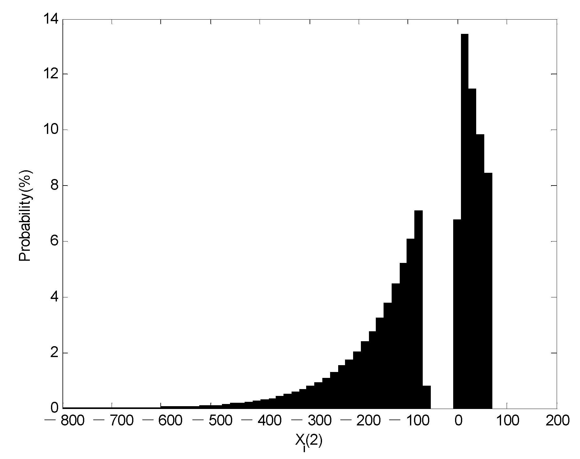
For simplicity, this paper tests the static character of a particle in one-dimensional space since the multidimensional variable can be formed by multi and independent one-dimensional variables. Some parameters take the following values: mbest = 0, Pi = 0, Xi(1) = 100, and α = 1. According to Equation (41), we test Xi(2) 100,000 times at random and obtain the frequency distribution histogram of Xi(2) as shown in Figure 1.
Figure 1 illustrates:
- (1)
- The upward search ability of QPSO is limited because the probability of Xi(2) > 70 is zero. Meanwhile, the downward search ability of QPSO is limited because the probability of −70 < Xi(2) < 0 is zero. There are dead-band searching problems for QPSO and the dead zones vary with the number of iterations.
- (2)
- There is a higher convergence speed when the optimal solution is close to the lower boundary because the static character of QPSO is asymmetric on both sides of Pi and there is a lower convergence speed when the optimal solution is close to the upper boundary.
- (3)
- There are different dead zones for every iteration and a particle needs at least two iterations in order to search the dead-band space, which reduces the search ability and increases the number of iterations when the optimal solution is in the dead-band space.
Since every dimension has dead zones during the iteration of every multi-dimensional particle, the dead zones grow in size and number with the increase of dimensions. The search range of the population is the union of the search ranges of all particles while iterating. When a particle has less dimensions, the dead zones decrease in size and number, which makes it easier to cover the whole search space by the union of the search ranges of all particles, leading to better convergence performance of the algorithm. When the population size remains the same, the increased dimensions of a particle increase dead zones in size and number, which brings about the difficulty in achieving coverage for the whole search space by the union of the search ranges of all particles, causing worse convergence performance of the algorithm.
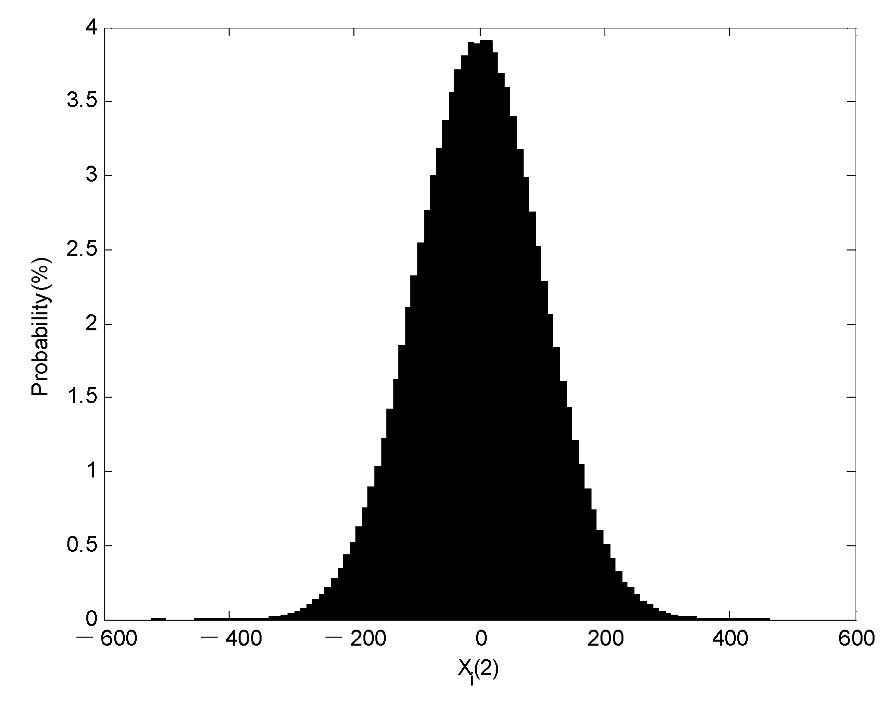
In order to enhance the convergence performance of QPSO, this paper proposes improvements in the static character since it suffers from the above analyzed shortcomings, meeting the following conditions:
- (1)
- There is no dead zone.
- (2)
- It is symmetric on both sides of Pi.
- (3)
- There is higher search probability in the neighborhood of Pi to guarantee the local search ability, and there is a certain search probability even if the space is far away from Pi to guarantee the global search ability by mutating.
In summary, in the proposed IQPSO method, Equation (41) is replaced by Equation (44) as follows:
4.3. Programming of IQPSO
The contraction-expansion coefficient α affects the convergence performance of QPSO. At the beginning of an iteration process, the algorithm must have the global search ability, and at the end of an iteration process, the algorithm must have the local search ability. To meet this requirement, α changes with the number of iterations as follows [28]:
The major steps are described as follows:
- (1)
- Some parameters are set such as ε, maxgen, M, and βz.
- (2)
- The population with the dimensions of Nt × Nj is initialized.
- (3)
- h is set equal to 1.
- (4)
- The fitness value CU(i) of particle i is calculated, according to Equation (25).
- (5)
- The best previous personal position Pbesti and the best personal fitness value fPbesti of particle i are obtained, and the global best position Gbest and the global best fitness value fGbest are obtained.
- (6)
- If max[CU(i)] − min[CU(i)] < ε or h = maxgen, it proceeds to step (11), otherwise to step (7).
- (7)
- Pi and mbest are calculated according to Equations (42) and (43).
- (8)
- α is calculated according to Equation (45).
- (9)
- The position of particle i is updated according to Equation (44).
- (10)
- h = h + 1, and then it proceeds to step (4).
- (11)
- The global best position Gbest and the global best fitness value fGbest are obtained.
5. Case Studies
5.1. Test System Data
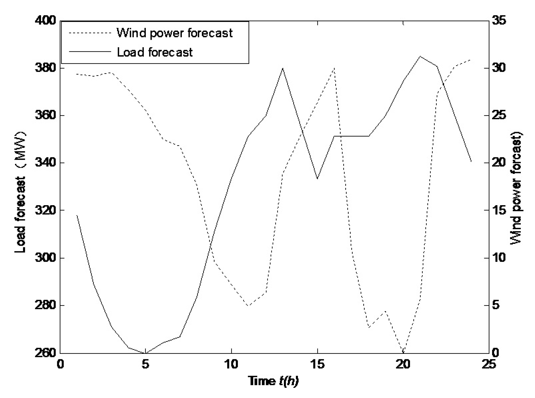
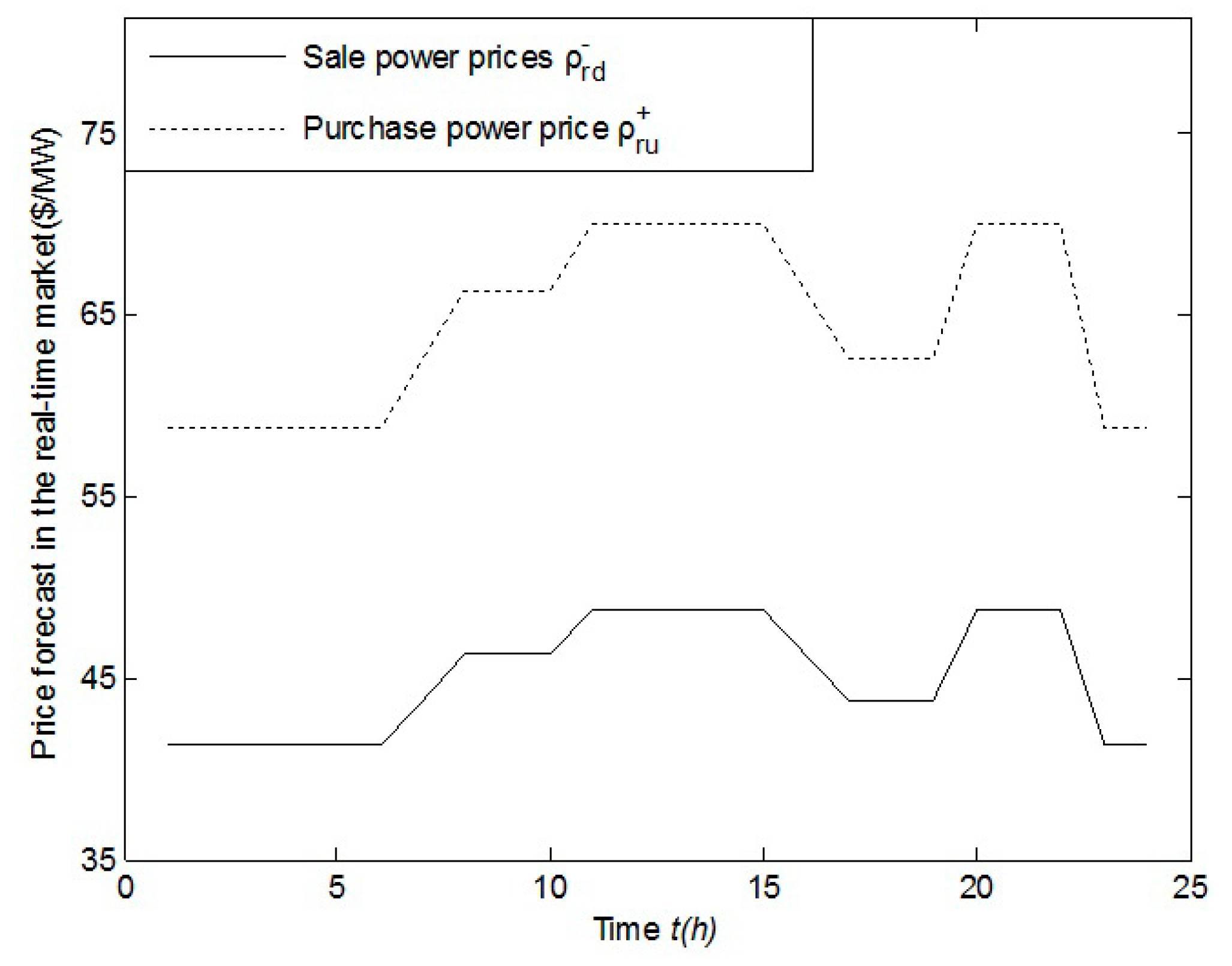
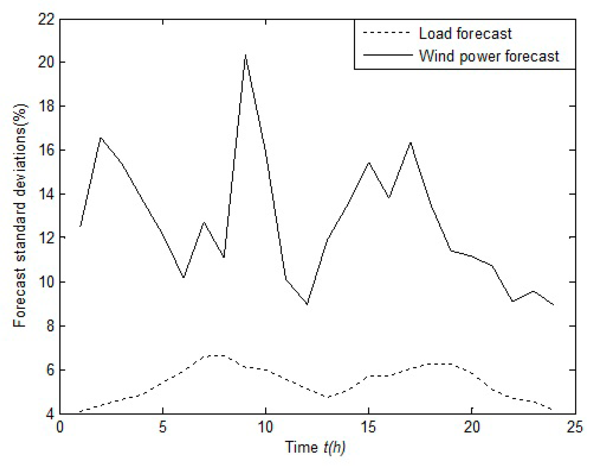
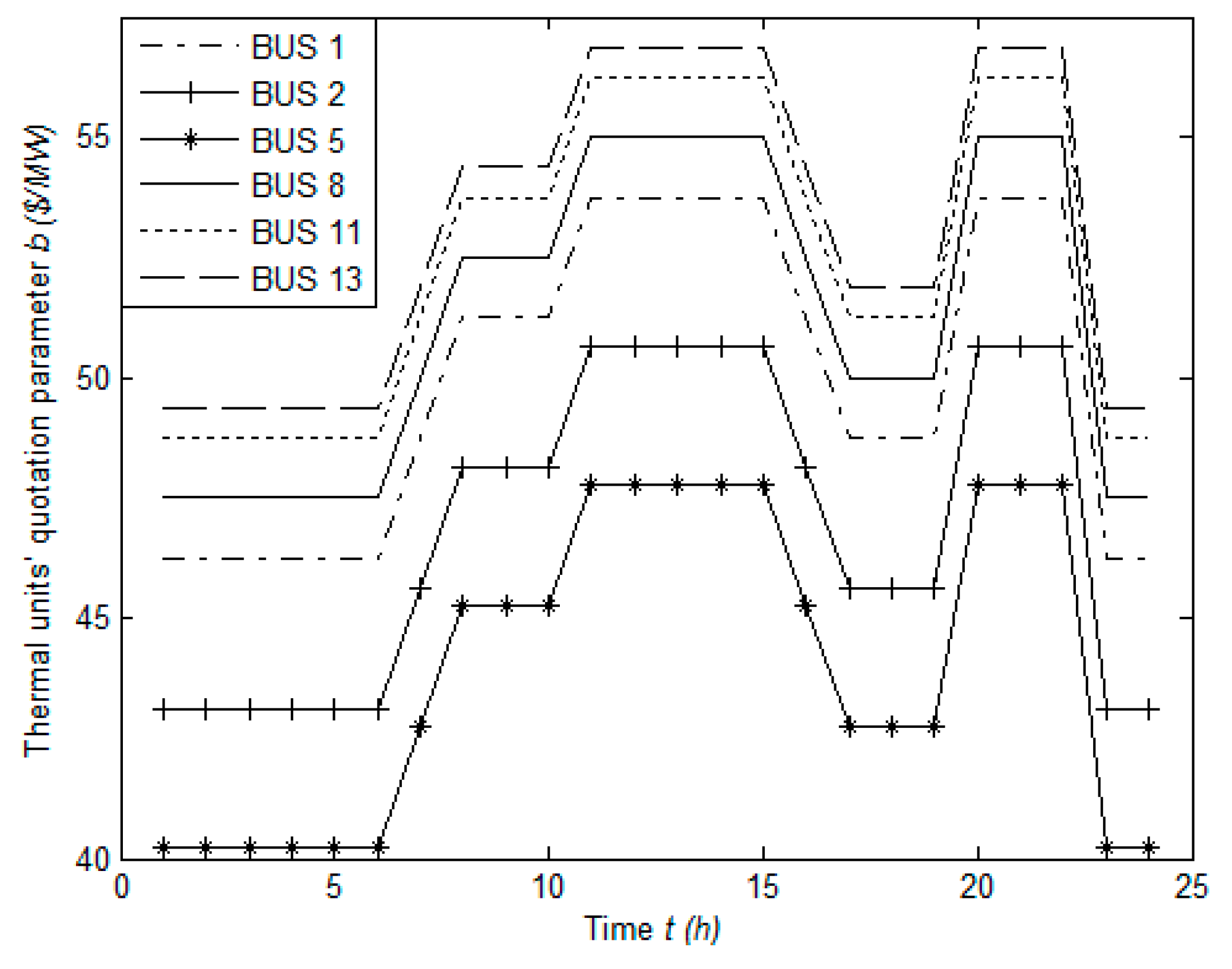
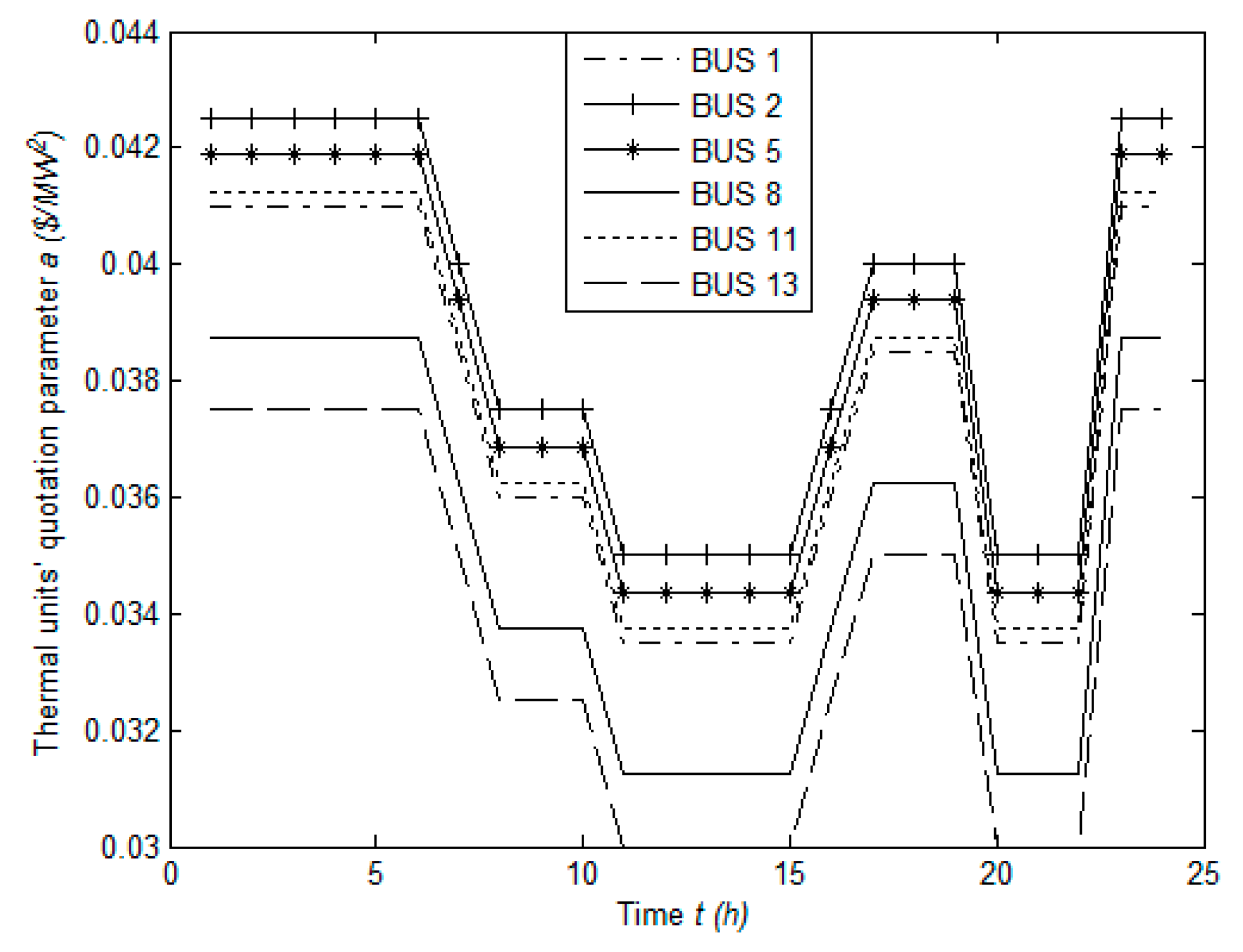
A numerical case for evaluating the proposed model and algorithm is performed on an IEEE 30-bus system. The thermal generators’ parameters are shown in Table 1. Hourly load forecast and wind power forecast are shown in Figure 3. Purchase and sale power average prices forecast in the real-time market are shown in Figure 4. Standard deviations of hourly load forecast and wind power forecast are shown in Figure 5. According to Equation (27), Γ = 28.1. Other parameters take the following values: er = 10%, βz = 0.98, maxgen = 2000, and M = 50. The thermal generators’ quotation function is given as follows:
where bj(t) and aj(t) are shown in Figure 6 and Figure 7, respectively.
5.2. Algorithm Comparison
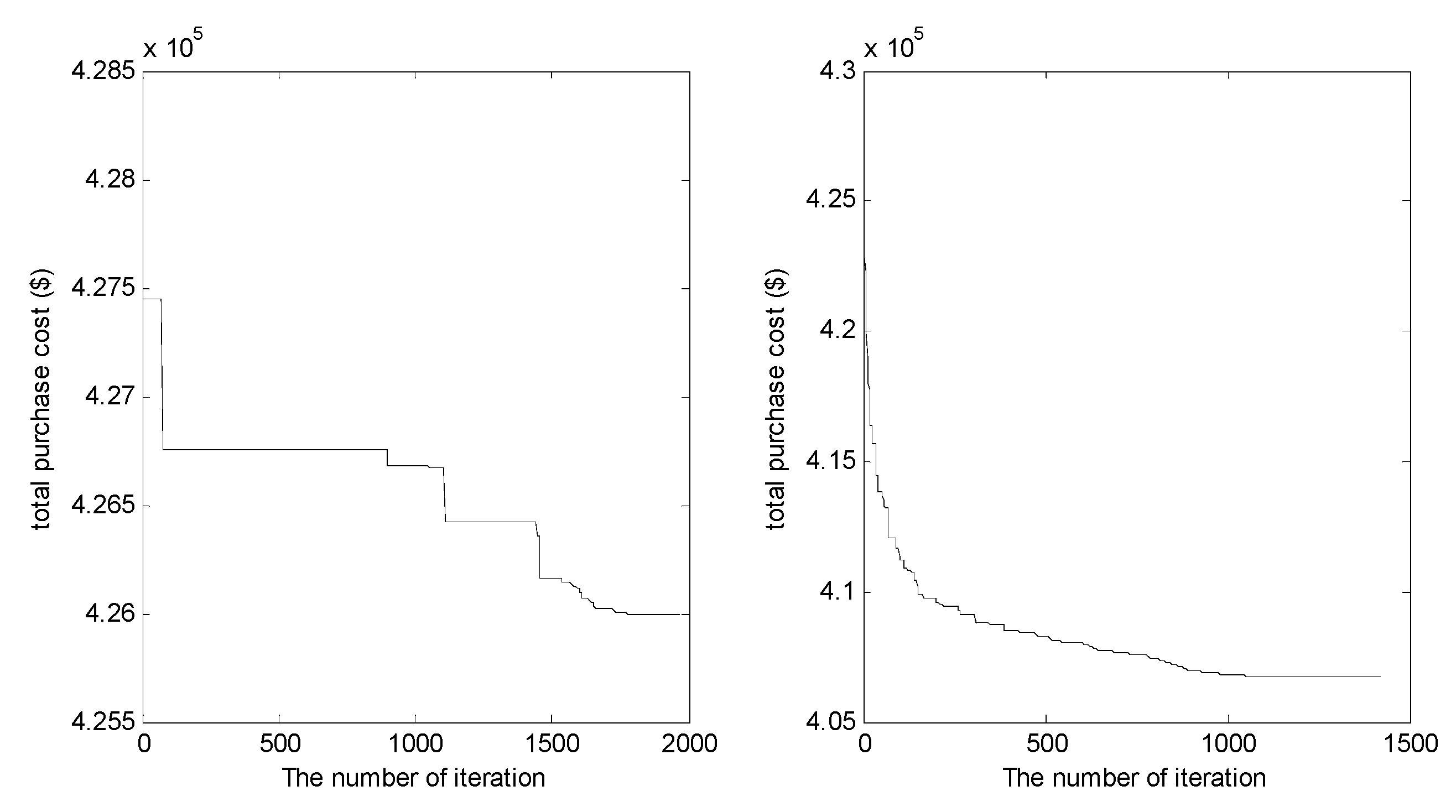
According to the above robust optimization model and case parameters, the results are shown in Table 2 with a comparison between QPSO and IQPSO.
Figure 8 visualizes the convergence process of QPSO on the left-hand side and IQPSO on the right-hand side. It can be seen that IQPSO has the better global search ability while QPSO is trapped in the local optimum.
5.3. Comparison of Purchase Power in the Day-Ahead Market for the Unified and Separate Trading
The optimal purchase power schedule for the unified and separate trading schemes in the day-ahead market is shown in Table 3 with IQPSO applied to achieving the optimal solutions. In Table 3, UT is short for the unified trading and ST is short for the separate trading. On the basis of the above parameters, the hourly total purchase power (t) is less when applying UT than the amount (t) when applying ST.
5.4. Impact Analysis of Price Forecast in the Real-Time Market
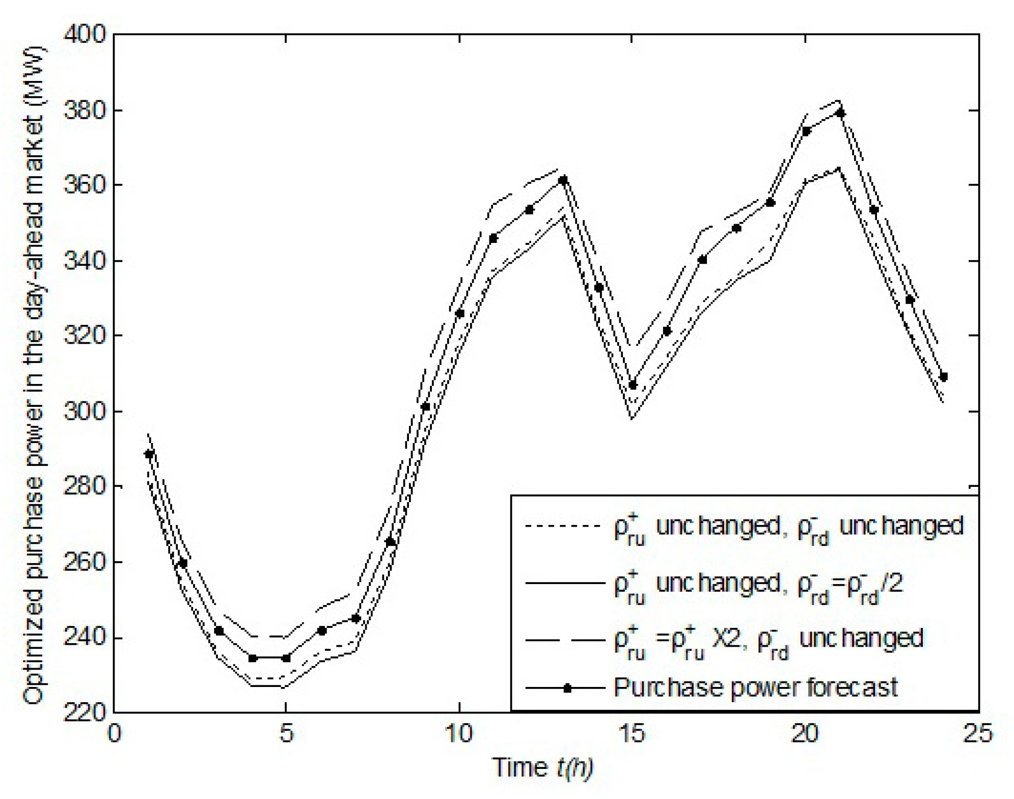
The comparison between (t) and (t) in the day-ahead market is further shown in Figure 9 with different prices in the real-time market.
The comparison between (t) (dotted line) and (t) (solid line with dot) is shown in the baseline scenario as explained in Figure 4, where (t) < (t), as seen in Table 3. Following an increase of the purchase power prices in the real-time market, the re-derived (t) (dashed line) becomes higher than the baseline value (t). While increasing the sale power prices in the real-time market, the re-derived (t) (solid line) is lower than (t) and (t) (dotted line).
5.5. Impact of σr, Γ, er
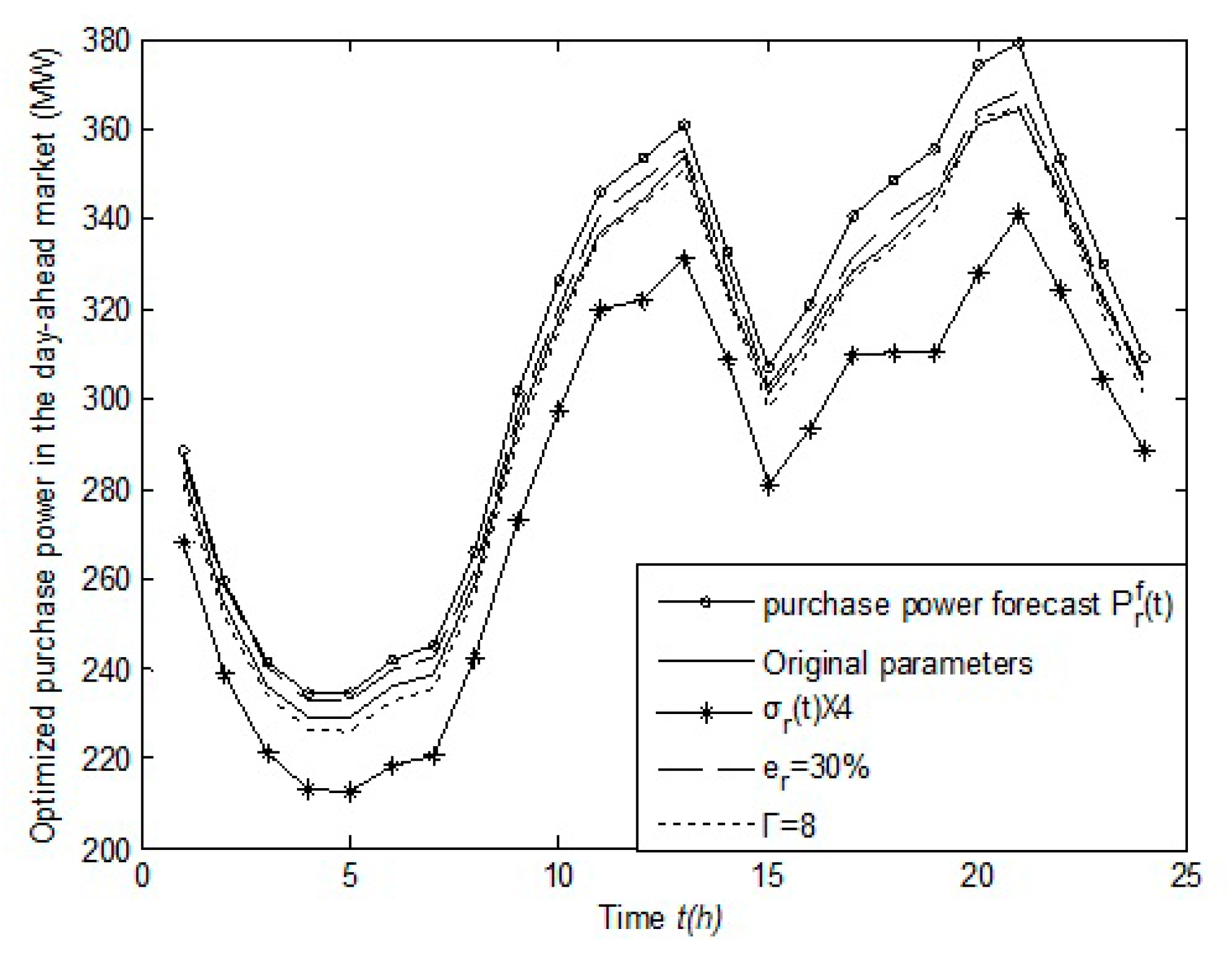
As the robust optimization focuses on the worst performance of the real-time market, the total purchase cost of the real-time market will increase when increased er (i.e., the price forecast deviation ratio at time t in the real-time market) makes the purchase environment worse; meanwhile, the total sale revenue of the real-time market will decline so that the purchase power strategies of the day-ahead market are more conservative, which reduces the difference between (t) (solid line with circle ) and (t) (dashed line) when er increases, according to Figure 10.
The decrease of Γ reduces the confidence level βz and facilitates the better economic environment of the real-time market, which increases the difference between (t) and (t) (dotted line), leaving more power for trading in the real-time market.
According to Figure 9, (t) < (t) when (t) and (t) remain unchanged, showing that the economic environment for selling power is worse than for purchasing power in the real-time market, so that it is necessary to reduce (t) (solid line with star) in order to reduce the sale power in the real-time market with the increase of σr(t). On the other hand, the power for trading in the real-time market increases because the increase of σr(t) reduces the accuracy of the purchase power forecast. For these two reasons, the difference between (t) and (t) (solid line with star) increases (i.e., (t) decreases) with the increase of σr(t), as illustrated in Figure 10.
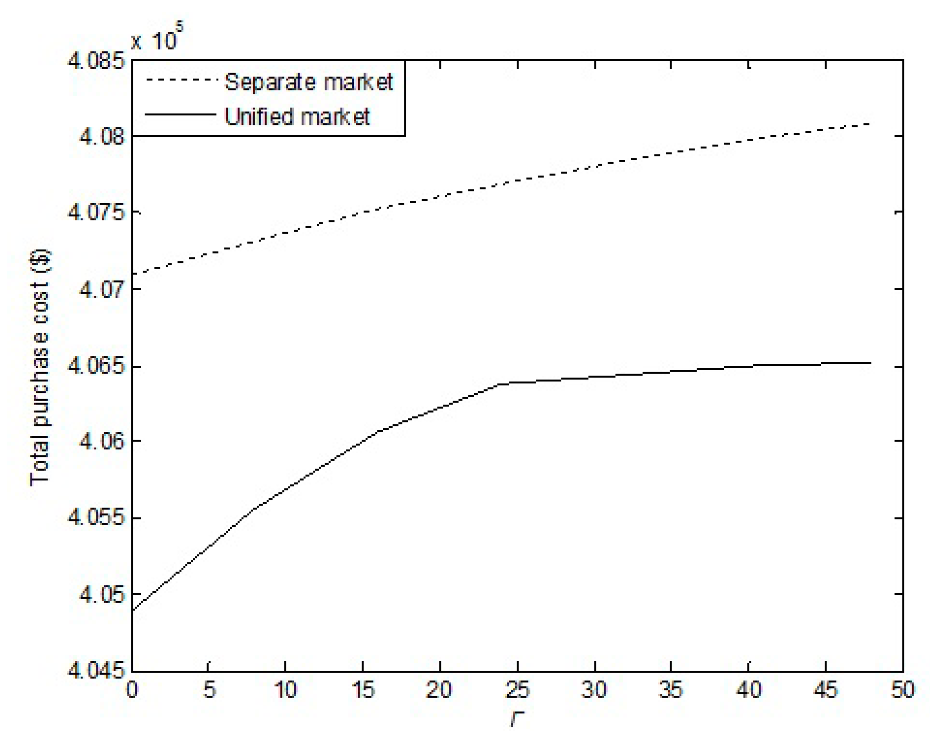
The impact of Γ on the total purchase power cost is shown in Figure 11, which shows that the total cost of the separate trading scheme (dotted line) is higher than the unified trading scheme (solid line).
The increase of Γ increases the total costs because the stronger robustness and the higher confidence level βz lead to considering worse scenarios. In addition to that, it can be seen that the growth rate of the total cost of the unified trading becomes slower with the increase of Γ. According to Figure 9, (t) < (t) when (t) and (t) are kept the same as the prices in Figure 4, which shows that a portion of the purchase power is transferred to the real-time market from the day-ahead market, leaving more power to be purchased and less power to be sold in the real-time market. In this case, the impact of on the total cost is bigger than the impact of . The robust optimization works in the worst case of the real-time market, which will firstly consider the highest so that the total cost increases quickly until reaches the maximum and then a smaller is taken into account in the robust optimization while Γ continues to increase. As mentioned above, the total cost is less affected when the sale power is reduced, resulting in the curve slowing down at the end.
In separate trading, the impact of the economic environment for purchasing power on the total cost is the same as that for the selling power because the power forecast errors are symmetrical, which leads to a smoother cost curve.
The total costs are shown in Table 4 when σr is multiplied based on the data in Figure 5 and Γ = 28.1.
In Table 4 above:
As shown in Table 4, the increase of σr leads to the increase of both the total cost and the reduction ratio of cost. For the increase of the total cost, this is because the low power forecast accuracy results in more power for trading increases in the real-time market. For the reduction ration of cost, there are two reasons. Firstly, in the separate trading scheme, the energy trading is performed according to (t) and the purchase cost is fixed in the day-ahead market in any case, but the power for trading increases greatly in the real-time market with the increase of σr, making the total cost of the separate trading increase quickly in light of ; Secondly, in the unified trading model, the energy trading is implemented based on (t) in the day-ahead market and the power for trading increases slowly in the real-time market with the increase of σr, which leads to less cost increase in the unified trading than that in the separate trading. In view of the above analysis, the unified trading model is superior to the separate trading model with the increase of σr. In particular, the unified trading model is more advantageous when large-scale wind power is integrated into the grid.
As is seen in Figure 10, the difference between (t) and (t) decreases with the increase of er, meaning that the total cost of the unified trading is closer to the total cost of the separate trading. Table 5 reports that the unified trading model with robust optimization is less advantageous because the economic environment for purchasing power is worse in the real-time market with the increase of er.
6. Conclusions
The day-ahead and real-time markets are combined to form a unified trading scheme with wind power integration in this paper. The robust optimization model is adopted by taking into account the uncertainty of the real-time market prices, load, and wind power, and then IQPSO is proposed to solve the optimization problem. The conclusions are as follows:
- The unified trading model based on robust optimization can optimize the purchase power in the day-ahead market and reduce the total cost for the two markets, which shows it is superior to the separate trading model due to large-scale wind power connected into the power systems.
- It is proven that the IQPSO has a higher convergence speed and stronger global search ability when compared with the standard QPSO.
In addition, the impact analysis of each parameter is summarized as follows:
- ♦
- The strategy of purchasing power in the day-ahead market is directly affected by the real-time price. The optimized purchase power will increase in the day-ahead market with higher purchase power prices and lower sale power prices in the real-time market and vice versa.
- ♦
- The unified trading model is superior when the power forecast errors become greater.
- ♦
- The lower the accuracy of the real-time market prices forecast, the worse the economic environment of the real-time market is. This reduces the economic efficiency of the unified trading model because the purchase strategy in the day-ahead market is more conservative.
- ♦
- The economic efficiency of the unified trading model is degraded when the confidence level is higher with the increase of the uncertain operator Γ. We can use the rational value of Γ to improve the economic efficiency as much as possible, following the requirement of the confidence level.
A direction for further research will consider the units’ startup and shutdown for the unified trading model and apply algorithms such as PSO, benders decomposition [20,29], genetic algorithm, and so on to solve the above optimization problem with comparisons in terms of the optimality, efficiency, and scalability.
Author Contributions
Yuewen Jiang conceived of the project and proposed the methodological framework and implementation roadmap; Meisen Chen performed the simulations; Shi You reviewed and improved the methodological framework. All authors discussed and approved of the simulation results. Yuewen Jiang mainly wrote this paper.
Conflicts of Interest
The authors declare no conflict of interest.
Nomenclature
| Indices | |
| t Index of time periods | Running from 1 to Nt, 1 h for every time period |
| j Index of dispatchable generators | Running from 1 to Nj |
| l Index of line | Running from 1 to L |
| m, n | Index of bus of line l |
| Decision Variables | |
| (t) | Optimized purchase power at time t in the day-ahead market |
| Pj(t) | Power purchase schedule for dispatchable generator j at time t in the day-ahead market |
| (t)/(t) | Upward/downward regulating power for generator j at time t in the real-time market |
| Other Variables | |
| Load forecast error at time t in the day-ahead market | |
| Wind power forecast error at time t in the day-ahead market | |
| / | Real load/real wind power at time t |
| / | Load forecast/wind power forecast standard deviation at time t in the day-ahead market |
| / | Load forecast/wind power forecast at time t in the day-ahead market |
| Imbalance power at time t in the real-time market | |
| (t) | Purchase power forecast at time t in the day-ahead market |
| CD | Purchase cost in the day-ahead market |
| Day-ahead market clearing price at time t | |
| / | Revenue/purchase cost in the real-time market |
| / | Purchase power/sale power price at time t in the real-time market |
| ΔPr(t)+/ΔPr(t)− | Power shortage/power surplus expectation at time t in the real-time market |
| β+(t)/β−(t) | Probability of ‘upward regulation’/‘downward regulation’ at time t in the real-time market |
| Difference between purchase power forecast and the optimized purchase power at time t | |
| Imbalance power standard deviation in the unified trading scheme at time t | |
| Total cost of the unified trading | |
| z = z+(t), z−(t) | Random variables in [–1, 1] |
| μz | Mean value of interval variables z+(t) and z−(t) |
| σz | Standard deviation of interval variables z+(t) and z−(t) |
| Vm/Vn | Voltage magnitudes at bus m/bus n of line l |
| θmn | Difference of voltage phase-angle between at bus m and bus n of line l |
| μ(h) | Random variable for the hth iteration in [0, 1] |
| Xi(h) | Position of particle i for the hth iteration |
| Pi | Center of the potential well |
| h | Number of current iterations |
| Random variable in [0, 1] | |
| mbest | Central position of personal best positions |
| Pbesti | Personal best position of particle i |
| Gbest | Global best position |
| Stochastic variable with standard normal distribution | |
| Constants and Parameters | |
| er | Deviation ratio to the expected price in the real-time market |
| / | Deviation from the expected price at time t in the real-time market |
| / | Purchase power/sale power expected price at time t in the real-time market |
| Γ | Degree of uncertainty for random variables |
| J | Number of interval variables z+(t) and z−(t) |
| / | Minimum/maximum capacity of the dispatchable generator j |
| / | Ramp down/up rate limit of the generator j |
| Upper limit for power flow of line l | |
| gmn/bmn | Conductance/susceptance of line l |
| M | Population size |
| α | Contraction-Expansion Coefficient |
| ε | Convergence accuracy |
| βz | Interval confidence level |
| maxgen | Maximum number of iterations |
| aj(t), bj(t) | Thermal generators’ quotation parameters of generator j at time t |
References
- Aparicio, N.; MacGill, I.; Abbad, J.R.; Beltran, H. Comparison of wind energy support policy and electricity market design in Europe, the United States, and Australia. IEEE Trans. Sustain. Energy 2012, 3, 809–818. [Google Scholar] [CrossRef]
- Martín, S.; Smeers, Y.; Aguado, J.A. A stochastic two settlement equilibrium model for electricity markets with wind generation. IEEE Trans. Power Syst. 2015, 30, 1–13. [Google Scholar] [CrossRef]
- Abbaspourtorbati, F.; Conejo, A.; Wang, J.; Cherkaoui, R. Pricing electricity through a stochastic non-convex market-clearing model. IEEE Trans. Power Syst. 2017, 32, 1248–1259. [Google Scholar] [CrossRef]
- Gil, H.A.; Lin, J. Wind power and electricity prices at the PJM market. IEEE Trans. Power Syst. 2013, 28, 3945–3953. [Google Scholar] [CrossRef]
- Yousefi, A.; Iu, H.H.C.; Fernando, T.; Trinh, H. An approach for wind power integration using demand side resources. IEEE Trans. Sustain. Energy 2013, 4, 917–924. [Google Scholar] [CrossRef]
- Papavasiliou, A.; Oren, S.S. Large-scale integration of deferrable demand and renewable energy sources. IEEE Trans. Power Syst. 2014, 29, 489–499. [Google Scholar] [CrossRef]
- Khodayar, M.E.; Manshadi, S.D.; Wu, H.; Lin, J. Multiple period ramping processes in day-Ahead electricity markets. IEEE Trans. Sustain. Energy 2016, 7, 1634–1645. [Google Scholar] [CrossRef]
- Wu, H.; Shahidehpour, M.; Li, Z.; Tian, W. Chance-constrained day-ahead scheduling in stochastic power system operation. IEEE Trans. Power Syst. 2014, 29, 1583–1591. [Google Scholar] [CrossRef]
- Hu, B.; Wu, L.; Marwali, M. On the robust solution to SCUC with load and wind uncertainty correlations. IEEE Trans. Power Syst. 2014, 29, 2952–2964. [Google Scholar] [CrossRef]
- Yuewen, J.; Buying, W. Real-time market dispatch based on ultra-short-term forecast error of wind power. Electr. Power Autom. Equip. 2015, 35, 12–17. (In Chinese) [Google Scholar]
- Wang, Q.; Zhang, C.; Ding, Y.; Xydis, G.; Wang, J.; Østergaard, J. Review of real-time electricity markets for integrating distributed energy resources and demand response. Appl. Energy 2015, 138, 695–706. [Google Scholar] [CrossRef]
- Farahmand, H.; Aigner, T.; Doorman, G.L.; Korpas, M.; Huertas-Hernando, D. Balancing market integration in the Northern European continent: A 2030 case study. IEEE Trans. Sustain. Energy 2012, 3, 918–930. [Google Scholar] [CrossRef]
- Dai, T.; Qiao, W. Optimal bidding strategy of a strategic wind power producer in the short-term market. IEEE Trans. Sustain. Energy 2015, 6, 207–219. [Google Scholar] [CrossRef]
- Liu, G.; Xu, Y.; Tomsovic, K. Bidding strategy for microgrid in day-ahead market based on hybrid stochastic/robust optimization. IEEE Trans. Smart Grid 2016, 7, 227–237. [Google Scholar] [CrossRef]
- Reddy, S.S.; Bijwe, P.R.; Abhyankar, A.R. Optimal posturing in day-ahead market clearing for uncertainties considering anticipated real-time adjustment costs. IEEE Syst. J. 2015, 9, 177–190. [Google Scholar] [CrossRef]
- Bai, H.; Miao, S.; Ran, X.; Ye, X. Optimal dispatch strategy of a virtual power plant containing battery switch stations in a unified electricity market. Energies 2015, 8, 2268–2289. [Google Scholar] [CrossRef]
- Conejo, A.J.; Morales, J.M.; Martinez, J.A. Tools for the analysis and design of distributed resources-part III: Market studies. IEEE Trans. Power Deliv. 2011, 16, 1663–1670. [Google Scholar] [CrossRef]
- Fanzeres, B.; Street, A.; Barroso, L.A. Contracting strategies for renewable generators: A hybrid stochastic and robust optimization approach. IEEE Trans. Power Syst. 2015, 30, 1825–1837. [Google Scholar] [CrossRef]
- Baughman, M.L.; Lee, W.W. A Monte Carlo model for calculating spot market prices of electricity. IEEE Trans. Power Syst. 1992, 7, 584–590. [Google Scholar] [CrossRef]
- Bertsimas, D.; Litvinov, E.; Sun, X.A.; Zhao, J.; Zheng, T. Adaptive robust optimization for the security constrained unit commitment problem. IEEE Trans. Power Syst. 2013, 28, 52–63. [Google Scholar] [CrossRef]
- Wu, L.; Shahidehpour, M.; Li, Z. Comparison of scenario-based and interval optimization approaches to stochastic SCUC. IEEE Trans. Power Syst. 2012, 27, 913–921. [Google Scholar] [CrossRef]
- Bo, R.; Li, F. Impact of load forecast uncertainty on LMP. In Proceedings of the 2009 Power Systems Conference and Exposition, Seattle, WA, USA, 15–18 March 2009; pp. 1–6. [Google Scholar]
- Doherty, R.; O’Malley, M. A new approach to quantify reserve demand in systems with significant installed wind capacity. IEEE Trans. Power Syst. 2005, 20, 587–595. [Google Scholar] [CrossRef]
- Bertsimas, D.; Sim, M. The price of robustness. Oper. Res. 2004, 52, 35–53. [Google Scholar] [CrossRef]
- Vlachogiannis, J.G.; Lee, K.Y. A comparative study on particle swarm optimization for optimal steady-state performance of power systems. IEEE Trans. Power Syst. 2006, 21, 1718–1728. [Google Scholar] [CrossRef]
- Meng, K.; Wang, H.G.; Dong, Z.Y.; Wong, K.P. Quantum-inspired particle swarm optimization for valve-point economic load dispatch. IEEE Trans. Power Syst. 2010, 25, 215–222. [Google Scholar] [CrossRef]
- Sun, J.; Feng, B.; Xu, W. Particle swarm optimization with particles having quantum behavior. In Proceedings of the 2004 Congress on Evolutionary Computation, Portland, OR, USA, 19–23 June 2004; Volume 1, pp. 325–331. [Google Scholar]
- Huang, W.Y.; Xu, X.J.; Pan, X.B.; Sun, Y.J.; Li, S. Control strategy of contraction-expansion coefficient in quantum-behaved particle swarm optimization. Appl. Res. Comput. 2016, 33, 2592–2595. (In Chinese) [Google Scholar]
- Zhao, L.; Zeng, B. Robust unit commitment problem with demand response and wind energy. In Proceedings of the 2012 IEEE Power and Energy Society General Meeting, San Diego, CA, USA, 22–26 July 2012; pp. 1–8. [Google Scholar]
Figure 1.
Frequency distribution histogram of Xi(2).

Figure 2.
Improved frequency distribution histogram of Xi(2).

Figure 3.
Hourly load and wind power forecasts.

Figure 4.
Purchase and sale power price forecasts in the real-time market.

Figure 5.
Standard deviations of the hourly load forecast and wind power forecast.

Figure 6.
Thermal generators’ quotation parameter bj(t).

Figure 7.
Thermal generators’ quotation parameter aj(t).

Figure 8.
Convergence curves of the two algorithms (QPSO left IQPSO right).

Figure 9.
Impact of real-time prices on (t) in the day-ahead market.

Figure 10.
(t) in the day-ahead market when σr, Γ, and er change, respectively.

Figure 11.
The impact of Γ on the total cost.


Table 1.
Parameters of the thermal generators.
| Generator Bus | 1 | 2 | 5 | 8 | 11 | 13 |
|---|---|---|---|---|---|---|
| Maximum capacity (MW) | 200 | 80 | 50 | 35 | 30 | 40 |
| Minimum capacity (MW) | 80 | 30 | 15 | 10 | 12 | 18 |
Table 2.
Optimal total cost of the two algorithms.
| Algorithms | Optimal Total Cost ($) | The Number of Iterations |
|---|---|---|
| QPSO | 4.260 × 10⁵ | 2000 |
| IQPSO | 4.064 × 10⁵ | 1447 |
Table 3.
Hourly optimal purchase power for the unified and separate trading in the day-ahead market (MW).
Table 3.
Hourly optimal purchase power for the unified and separate trading in the day-ahead market (MW).
| Hour | UT BUS1 | ST BUS1 | UT BUS2 | ST BUS2 | UT BUS5 | ST BUS5 | UT BUS8 | ST BUS8 | UT BUS 11 | ST BUS 11 | UT BUS 13 | ST BUS 13 | UT TOTAL | ST TOTAL |
|---|---|---|---|---|---|---|---|---|---|---|---|---|---|---|
| 1 | 89.62 | 87.74 | 68.94 | 70.32 | 49.81 | 49.60 | 27.13 | 34.76 | 29.91 | 28.08 | 18.00 | 18.00 | 283.4 | 288.5 |
| 2 | 87.94 | 89.28 | 79.97 | 55.10 | 25.84 | 36.25 | 26.23 | 33.83 | 16.48 | 27.34 | 18.00 | 18.00 | 254.5 | 259.8 |
| 3 | 86.18 | 85.61 | 32.21 | 78.91 | 49.54 | 15.20 | 21.72 | 13.89 | 28.60 | 29.99 | 18.00 | 18.00 | 236.3 | 241.6 |
| 4 | 87.03 | 91.76 | 30.01 | 30.28 | 49.56 | 46.20 | 29.59 | 34.99 | 14.73 | 13.27 | 18.00 | 18.00 | 228.9 | 234.5 |
| 5 | 84.74 | 86.62 | 35.16 | 35.44 | 49.21 | 34.63 | 12.05 | 34.21 | 29.80 | 25.50 | 18.00 | 18.00 | 229.0 | 234.4 |
| 6 | 83.85 | 82.08 | 41.64 | 53.72 | 47.89 | 23.88 | 14.84 | 34.45 | 29.88 | 29.77 | 18.00 | 18.00 | 236.1 | 241.9 |
| 7 | 87.96 | 87.28 | 56.77 | 44.73 | 46.78 | 48.92 | 12.08 | 27.79 | 17.19 | 18.17 | 18.01 | 18.00 | 238.8 | 244.9 |
| 8 | 93.44 | 95.08 | 54.14 | 74.06 | 43.56 | 37.90 | 32.94 | 12.15 | 17.03 | 28.51 | 18.00 | 18.00 | 259.1 | 265.7 |
| 9 | 91.07 | 99.72 | 77.47 | 77.36 | 45.58 | 47.72 | 32.30 | 33.78 | 29.96 | 24.92 | 18.01 | 18.00 | 294.4 | 301.5 |
| 10 | 104.1 | 107.8 | 79.89 | 80.00 | 49.99 | 50.00 | 35.00 | 35.00 | 29.99 | 29.99 | 19.11 | 23.28 | 318.0 | 326.1 |
| 11 | 116.6 | 120.6 | 79.66 | 80.00 | 49.98 | 50.00 | 35.00 | 35.00 | 29.84 | 30.00 | 26.06 | 30.56 | 337.2 | 346.2 |
| 12 | 119.9 | 124.1 | 80.00 | 80.00 | 50.00 | 50.00 | 34.98 | 35.00 | 29.76 | 30.00 | 29.74 | 34.46 | 344.4 | 353.6 |
| 13 | 124.5 | 127.7 | 79.81 | 80.00 | 50.00 | 50.00 | 34.85 | 35.00 | 29.98 | 30.00 | 34.90 | 38.47 | 354.1 | 361.2 |
| 14 | 110.4 | 114.3 | 79.99 | 80.00 | 49.96 | 50.00 | 34.98 | 35.00 | 29.94 | 30.00 | 19.05 | 23.43 | 324.3 | 332.7 |
| 15 | 98.76 | 96.35 | 79.91 | 79.98 | 49.88 | 48.55 | 27.40 | 34.74 | 27.44 | 29.38 | 18.00 | 18.00 | 301.4 | 307.0 |
| 16 | 101.9 | 105.4 | 79.99 | 80.00 | 49.57 | 50.00 | 34.40 | 35.00 | 29.92 | 30.00 | 18.00 | 20.65 | 313.8 | 321.1 |
| 17 | 106.2 | 111.8 | 79.98 | 80.00 | 50.00 | 50.00 | 34.94 | 35.00 | 29.97 | 30.00 | 27.52 | 33.70 | 328.5 | 340.5 |
| 18 | 109.6 | 115.6 | 79.98 | 80.00 | 49.95 | 50.00 | 34.86 | 35.00 | 29.99 | 30.00 | 31.28 | 37.89 | 335.7 | 348.5 |
| 19 | 114.0 | 120.6 | 79.99 | 80.00 | 49.98 | 50.00 | 34.98 | 35.00 | 29.99 | 30.00 | 36.06 | 40.00 | 344.9 | 355.6 |
| 20 | 127.7 | 139.4 | 79.99 | 80.00 | 50.00 | 50.00 | 34.99 | 35.00 | 29.98 | 30.00 | 38.46 | 40.00 | 361.1 | 374.4 |
| 21 | 129.5 | 144.3 | 80.00 | 80.00 | 50.00 | 50.00 | 35.00 | 35.00 | 30.00 | 30.00 | 39.97 | 40.00 | 364.5 | 379.3 |
| 22 | 121.3 | 124.0 | 79.97 | 80.00 | 49.99 | 50.00 | 34.88 | 35.00 | 28.62 | 30.00 | 31.23 | 34.30 | 346.0 | 353.3 |
| 23 | 100.9 | 104.2 | 79.97 | 80.00 | 49.82 | 50.00 | 33.86 | 35.00 | 29.93 | 30.00 | 27.00 | 30.60 | 321.5 | 329.8 |
| 24 | 92.55 | 94.41 | 79.18 | 80.00 | 49.94 | 50.00 | 34.38 | 35.00 | 30.00 | 30.00 | 18.00 | 19.89 | 304.1 | 309.3 |
Table 4.
The impact of σr on the total costs.
| Multiple of σr | Total Cost of the Unified Trading (UTTC) ($) | Total Cost of the Separate Trading (STTC) ($ ) | Reduction Ratio of Cost (%) |
|---|---|---|---|
| 1 | 4.066 × 10⁵ | 4.078 × 10⁵ | 0.33 |
| 2 | 4.078 × 10⁵ | 4.103 × 10⁵ | 0.59 |
| 3 | 4.092 × 10⁵ | 4.127 × 10⁵ | 0.85 |
| 4 | 4.108 × 10⁵ | 4.152 × 10⁵ | 1.06 |
Table 5.
Impact of er on the total purchase costs.
| er (%) | Total Cost of the Unified Trading ($ ) | Total Cost of the Separate Trading ($ ) | Reduction Ratio of Cost (%) |
|---|---|---|---|
| 10 | 4.066 × 10⁵ | 4.078 × 10⁵ | 0.33 |
| 20 | 4.077 × 10⁵ | 4.085 × 10⁵ | 0.20 |
| 30 | 4.088 × 10⁵ | 4.092 × 10⁵ | 0.11 |
| 40 | 4.096 × 10⁵ | 4.099 × 10⁵ | 0.07 |
© 2017 by the authors. Licensee MDPI, Basel, Switzerland. This article is an open access article distributed under the terms and conditions of the Creative Commons Attribution (CC BY) license (http://creativecommons.org/licenses/by/4.0/).
Share and Cite
MDPI and ACS Style
Jiang, Y.; Chen, M.; You, S. A Unified Trading Model Based on Robust Optimization for Day-Ahead and Real-Time Markets with Wind Power Integration. Energies 2017, 10, 554. https://doi.org/10.3390/en10040554
AMA Style
Jiang Y, Chen M, You S. A Unified Trading Model Based on Robust Optimization for Day-Ahead and Real-Time Markets with Wind Power Integration. Energies. 2017; 10(4):554. https://doi.org/10.3390/en10040554
Chicago/Turabian StyleJiang, Yuewen, Meisen Chen, and Shi You. 2017. "A Unified Trading Model Based on Robust Optimization for Day-Ahead and Real-Time Markets with Wind Power Integration" Energies 10, no. 4: 554. https://doi.org/10.3390/en10040554
Note that from the first issue of 2016, this journal uses article numbers instead of page numbers. See further details here.