1. Introduction
Wireless sensor networks (WSN) can be used to collect data of interest with high spatial and temporal resolution. Such networks are made up of nodes consisting of the required sensors, wireless communications hardware, energy storage, and a microprocessor to facilitate data processing and other tasks [
1]. When outfitted with energy harvesting devices, these sensor nodes can be deployed without the need for large power supplies or frequent maintenance visits. This is of particular interest for long-term deployment in remote locations where trips to the field may be prohibitively expensive, impossible, or otherwise troublesome. Additionally, especially in environmental monitoring applications, certain energy sources are undesirable (e.g., large lead acid batteries that are difficult to transport) and therefore cannot be utilized to increase deployment length [
2]. Such applications include ecosystem monitoring in tropical dry forests, the arctic, and on glaciers [
3,
4,
5].
In order to realize the longest deployment possible while still collecting useful data, a node’s energy must be managed. There are a number of different methods of managing energy within WSNs. They can be divided into three different levels [
6]. At the component level, the choice of individual parts with low power operating modes and other similar optimizations are important for reducing the overall energy usage of the nodes. At the node level, adaptive duty cycling, as well as data transmission reducing schemes can be used to manage energy. Network level strategies include dynamic selection of network sinks and energy aware message routing to distribute energy usage intelligently [
7,
8,
9,
10]. The focus of this work is on the use of node level adaptive duty-cycling.
Without energy harvesting, duty-cycle based management is simple, as estimates of node energy usage and storage capacity can be used to directly determine its duty cycle. Management becomes more complex with the addition of harvesting, where differences in harvesting opportunities and limited storage necessitate striking a balance between energy conservation and consumption [
11]. On one side, liberal energy consumption runs the risk of missed measurements or outright node failure. On the other side, highly conservative energy management can lead to its inefficient use, e.g., when incoming energy can be neither used directly nor stored because the energy storage device is already full. With proper energy management, harvesting allows for smaller energy storage devices, as well as for longer deployment times, potentially approaching perpetual operation [
12].
Energy management strategies vary in complexity, based on the information available for decision making. Foreknowledge of harvesting opportunities may be included, e.g., extracted from the experienced harvesting opportunities. Adaptive duty cycling for energy-harvesting sensor nodes is discussed in [
13] with energy prediction based on an exponentially weighted average. The implemented controller allowed 58% more environmental energy utilization when compared to the case where power management is used without harvest awareness. Adaptation of sensor node parameters based on a prediction of future energy is shown in [
14]. There, the parameters are set based on the incoming energy, sensing rate and the usage of local memory. A power estimator based on the output of a numerical weather forecast model and integrated into a dynamic power management scheme is discussed in [
15]. This scheme affects energy intensive node operations, such as the duration of video transmitted back to the base station.
Fuzzy logic control is often used to implement adaptive duty cycling for individual nodes [
4,
6,
16]. Inputs to such fuzzy controllers generally include the state-of-charge of available energy storage devices, but may also include the amount of data stored on a node. Of particular interest to increasing usage of harvested energy is an input associated with energy forecast. Early estimates of incoming energy may allow for increased energy usage in cases when the incoming energy would support it, or to reduce energy consumption when a dearth of incoming energy is expected.
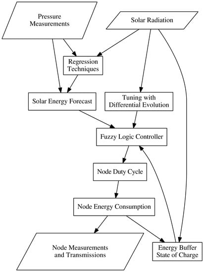
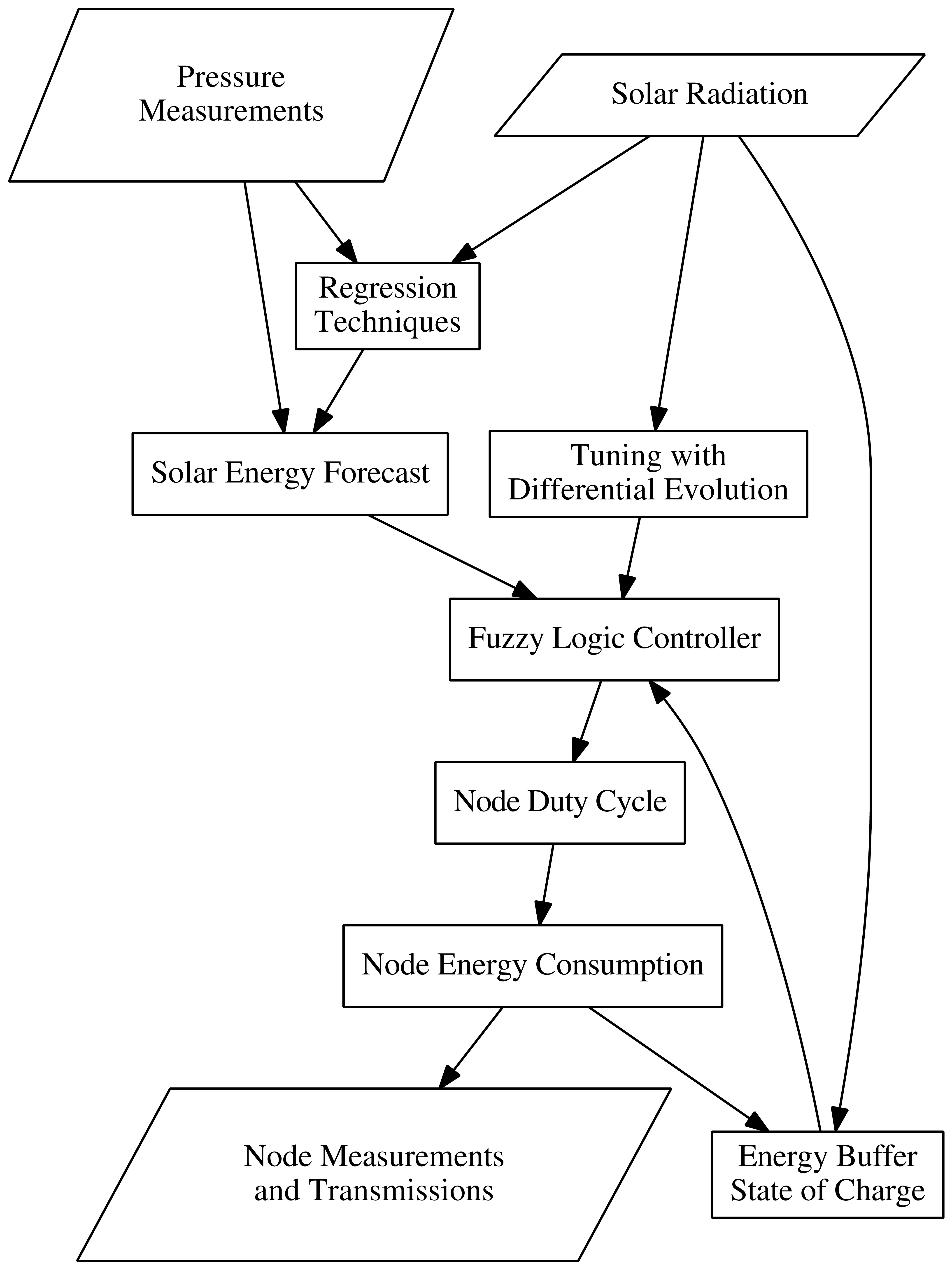
In this contribution, forecasts of daily solar energies are developed using measurements of atmospheric pressure. These forecasts are then combined with fuzzy logic controllers tuned using differential evolution. The ensuing system provides node-level energy management through adaptive duty cycling. This system was then applied to a simulation of a simple WSN in order to examine its behavior. While not fully representative of actual deployment conditions, simulations allow initial development of energy management strategies. The use of sophisticated simulation tools allows WSN development to occur faster and with lower costs compared to experimental trials with hardware prototypes. At the same time, they also provide repeatability that facilitates comparison between different strategies [
2]. This is especially important when applying optimization methods that require consistent approach to solution evaluation.
This paper is comprised of six sections. The materials and methods used are described in
Section 2.
Section 3 shows the development of a solar energy forecast based on measurements of atmospheric pressure. Design and optimization of the fuzzy logic controller is discussed in
Section 4. Results of simulations for a small wireless sensor network are presented in
Section 5. Major conclusions and potential directions of future work are outlined in
Section 6.
3. Energy Forecast
An energy forecast is an important component of an energy management scheme that allows to increase the amount of harvested energy used. With foreknowledge of harvesting opportunities, energy buffers may be depleted in advance of high amounts of incoming energy, or preserved if low amounts of energy are expected. Forecasts of daily solar energy have also become more important with the increased interest in renewable energy and smart agriculture. Tools for their modeling often require daily solar energy as an input. However, it may not have been measured due to the high cost of the required instrumentation [
36,
37,
38]. More common meteorological observations may be available and can be used to estimate the amounts of solar energy. These alternative methods usually make use of the difference between observed maximum and minimum daily temperatures, with some models including other variables (e.g., minimum relative humidity) to improve the estimates [
39,
40,
41,
42,
43]. Difficulty arises when applying regressions performed for one location to another, as differences in prevailing weather conditions may be quite significant.
With the limited hardware available in a sensor node, simple forecasts are preferable to more complex ones requiring intense computation. Additionally, meteorological variables useful for prediction of solar energy may not be required for the sensor nodes actual purpose, meaning that the inclusion of these values would require additional measurement instrumentation as well as energy expenditure and storage space that may not contribute to the main goal of the sensor network deployment.
In this work, we selected atmospheric as the predictor for solar energy forecasts, because of its relationship with changing weather conditions and cloud cover [
44]. Measurements of pressure have already been used for simple weather forecasts in consumer products for a number of years [
45,
46]. Proper measurement of this variable may also be simpler than others, e.g., siting requirements of temperature measurements require the instrument to be shaded and provided with adequate airflow [
47]. Additionally, appropriate sensors are available with low energy requirements (e.g., 2.7 mJ [
48]) when compared to some other sensors and other node operations [
2].
Creating the forecast begins by making an analytical estimate of the amount of incoming solar energy for a given location. The actual forecast target is an estimate of the transmissivity coefficient associated with cloud cover,
. This forecast value is then multiplied by the analytical estimate of incoming daily solar energy,
, which can be calculated as [
49,
50]:
where
and
are, respectively, the sunrise and sunset angles of the location, while
G is an estimate of the incoming solar radiation given by:
where
N is the day of the year and
is the solar irradiance reaching the Earth at the edge of atmosphere.
A simple model of clear sky atmospheric transmissivity,
, is added to account for some of the absorption and scattering in the atmosphere:
where
h is the site elevation in meters [
51]. This model was developed through a linearization of Beer’s Law (see [
52]) with respect to elevation, and is valid for site elevations of less than 6000 m with relatively clean air. It ignores some of the more complex factors including water vapor and atmospheric contaminants, making it an ideal estimate for cases where this additional information is not available and the assumptions are reasonable. A site specific model may be used instead for increased accuracy, but it would require calibration that may not be possible in practice.
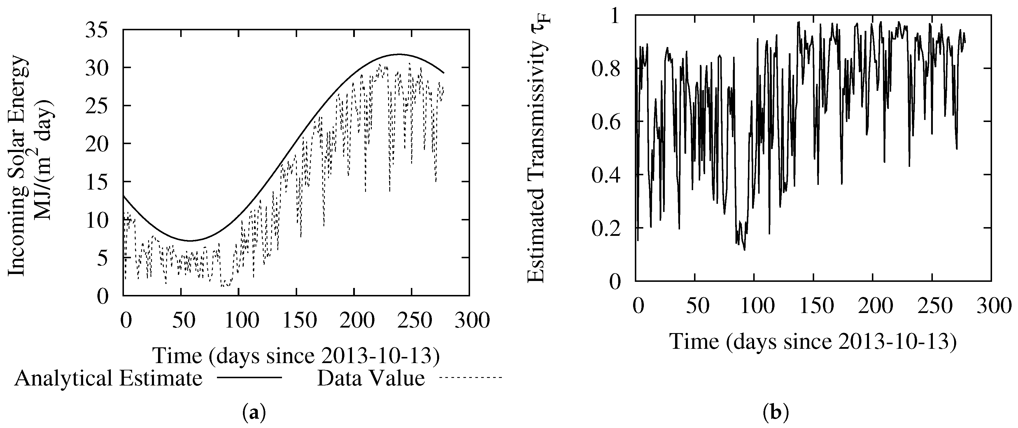
Dividing the measured daily solar energy by this analytical value, one can obtain an estimate of the transmissivity to be used as the forecast target,
. Samples of the measured incoming solar energy, the analytical estimate and the estimated transmissivity are shown in
Figure 1.
Using the calculated analytical estimate as the solar energy forecast for the different stations results in the mean absolute percentage errors (MAPE) and root mean squared errors (RMSE) shown in
Table 2.
For comparison purposes, an alternative possible model for estimating the incoming daily solar energy has been evaluated:
where
is the energy estimated using the Samandi-Hargreaves relationship,
is an empirical constant (a value of 0.17 is used here),
and
are the measured maximum and minimum temperatures of the day, and
is the analytical energy estimate [
41]. Applying this relationship to the available data sets for the prediction of the next-day solar energy resulted in the MAPE and RMSE values tabulated in
Table 3. These values are an improvement based on just using
as the predictor, both in terms of MAPE and RMSE.
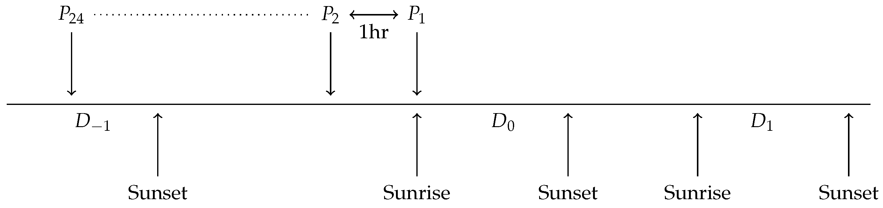
In our previous work, sets of pressure pairs and their differences were included as predictors, and only the energy for the upcoming day was predicted [
53]. Here, at sunrise of a given day
, the incoming solar energy for that day is predicted, as well as the incoming energy for the next five days (
,
, …,
). This approach is based on the most recent 24 hourly measurements (
,
, …,
), as shown in
Figure 2. The differences between the individual pressure measurements were calculated and supplied as inputs as well, since the change in pressure over time is considered a major indicator of weather changes.
In the previous exploration, there was no input corresponding either to the time of the year or to the expected amount of incoming energy. However, a dependence between the time of the year and the size of the prediction error was noted when longer time series were used. Attempting to lower these errors and improve the overall error metrics, the analytic estimate of the total incoming energy (Equation
1) was also provided as an input. Forecasts for the upcoming daylight hours (i.e.,
) and beyond (
and onwards) can also be made using the same measurements with , with the expectation that the longer forecasting horizon may improve performance of the controller to be developed later. However, because of the limited capacity of a sensor node’s energy buffer, there is expected to be a limit to the size of a useful forecasting horizon.
To design desired predictor, CART, RF, ELM, and MLP methods were used. The hidden layer sizes of the ELM and MLP neural networks were expanded to 50 nodes, and the maximum number of training iterations allowed for the network trained with backpropagation increased to 1000. The inputs for the neural network methods were scaled to , while the CART and RF inputs retained their original values. Models were trained on randomly selected training sets comprising 50% of the total available days. Ten trials were run for each prediction method and data set.
Trials were run for both cases where forecast models were created for each individual station, as well as for the case where all data was combined and used to create one model for all stations. Single tailed t-tests were used to compare the mean absolute errors of these forecasts and not found to provide a significant improvement. This could simplify deployment of WSN if this method were used for energy management.
Calculated MAPE values for
training set predictions for the various methods are shown in
Table 4, while RMSE values are shown in
Table 5. Selecting the trial runs with the lowest MAPE from the training set and applying them to the reserved test set yields the values shown in
Table 6. These error measures show that the NN based methods see larger increases in the error values than the tree based method when applied to the test set. Compared to the error values for these sites using the temperature measurements, the MAPE values were slightly higher, but the RMSE values were lower, meaning that there were fewer instances of large errors with these methods. This is an important finding, as larger errors can cause greater problems when used for energy management.
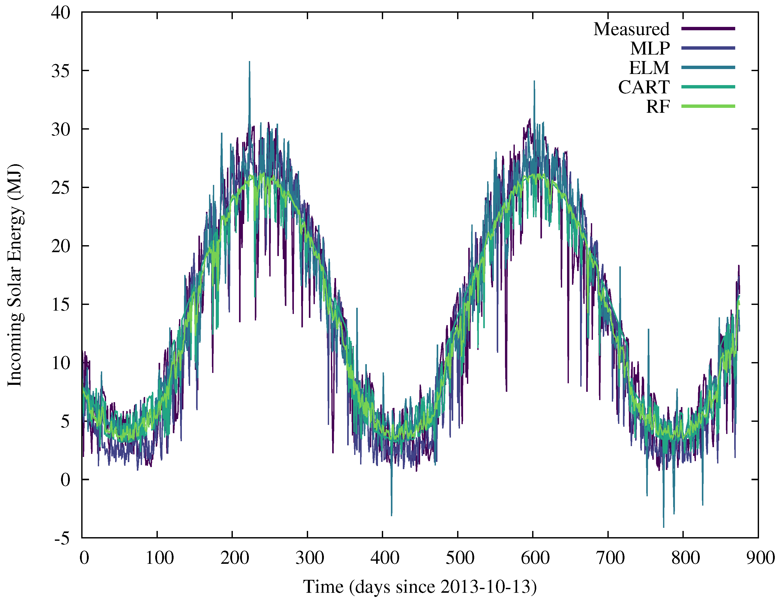
A time series of the predictions made for one of the stations is shown in
Figure 3. This figure shows that the CART and RF regressions have less deviation from the analytical estimate, while the NN methods had larger deviations. The ELM prediction had a number of impossible values, i.e., negative solar energies, that could be filtered out, but this is unlikely to make this method competitive.
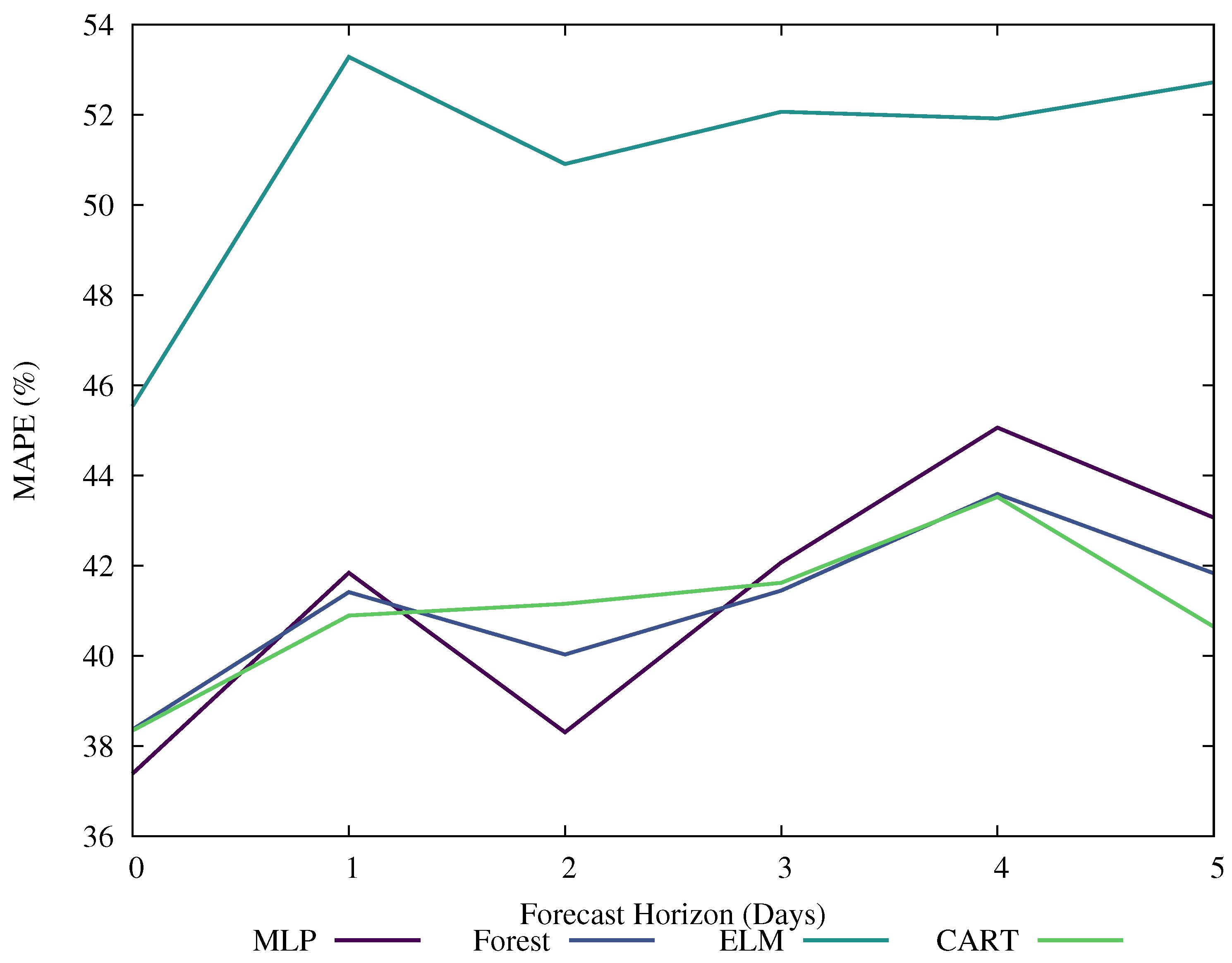
Figure 4 shows the test set results for models with the lowest MAPE values for larger forecasting horizons. With the increasing prediction time, the error values generally increased, as expected. Compared to the other methods, ELM had much higher error values for all forecasting horizons.
4. Controller Optimization
One strength of fuzzy logic is the ability to use linguistically meaningful terms to describe the system’s desired behavior, and to form the controller based on this description. However, the overall performance of the controller can be improved through optimization of the fuzzy membership functions. These functions are encoded as vectors of real valued numbers representing their individual parameters and operated on by an optimization method. In order to evaluate candidate solutions, the vectors are decoded into a fuzzy controller that is executed, and fitness values are calculated based on its performance.
After the randomization of the optimization algorithm, additional considerations should be made to ensure that a sound fuzzy controller is created. Preference for a semantically sound fuzzy set during optimization ensures consistency of the resulting controller and increases its transparency. Two important aspects of semantic soundness are coverage and distinguishability [
30]. Metrics related to these two aspects can be calculated and added to the fitness function.
Our previous work on optimization of similar controllers included 5 membership functions for each input [
54]. The resulting partitions for that optimization contained membership function with a large amount of overlap, leading to the selection of a lower number in the current work, i.e., 3 membership functions per input.
The membership functions of a fuzzy logic controller that determine the duty cycle of the sensor nodes were tuned using DE (c.f.
Section 2). The inputs for the candidate controllers were the state of the energy buffer, and either one or two days of future energy. The output of the controller was a node activity value,
, that was used to determine the number of operations a node attempted to complete in a day.
The time between measurements is allowed to vary from 60 to 3600 s (1 min–1 h), while the time between transmissions from 120 to 86,400 s (2 min–1 day). In these simulations,
is used to modulate both operations. The relationship between the number of operations occurring in a 24 h period,
O, and
is expressed using:
where
O may be either measurement or transmission. Selection of
and
is used as a simple way of ensuring that measurements of certain variables are made with a sufficient frequency. Two updates of node activities are performed, one at the sunrise of the current day and one at the sunset. For cases where energy forecasts are used, new forecasts are not made as part of the sunset update, but those made during the sunrise update are used if appropriate.
In order to compare the performances of candidate solutions, a fitness function,
f, is defined as:
where
represents unused environmental energy,
is the energy used from the primary battery reserves, and the final terms,
and
, represent penalties related to increasing the input variables distinguishability (i.e., that the membership functions do not overlap so much as to not be meaningfully unique) and coverage (i.e., that the entire input space is covered), respectively. Scaling constants
a,
b and
c define the relative importance of the individual fitness components. In this work,
is defined as the energy present in the environment that is neither immediately used, nor stored for future use. That is, energy that is not harvested because the energy buffer is already full and the node operates at its highest activity level.
The relative importance of and in this fitness function depends on a number of factors, including the length of desired deployment, the expected amount of energy available for harvest, and the value of individual measurements. For this particular case, a has been set to since the typical amount of uncaptured and unused energy from previous simulations is on the order of 1 MJ. The reserve battery usage has a relatively high weight, . To encourage formation of meaningful fuzzy sets, c is set to a value of 5.
Energy values used for energy costs of various operations, including energy usage estimates for transmission, reception, and measurements, were taken from [
55]. Estimations of the energy used for prediction of daily solar energy [
56] were presented in [
57]. Different combinations of microcontroller, operating frequency, compilers and optimization levels were tested, resulting in power consumption ranging between 5.4
J and 5817.6
J with the bulk of the tested configurations requiring less than 100
J. As many of these energy estimates are below the estimated energy usage during sleep (56.67
J), the energy cost associated with the creation of an the energy forecast can be safely neglected.
The optimization was performed using a single location (Moxee) and the first 670 days of the 880 day data set. A single node was used in order to keep processing times low. This did remove a degree of interaction between nodes, as well as reduced the overall energy usage of the node as it did not receive any transmissions during this simulation. To compensate for the lower energy consumption, the cost of transmission was increased compared to the value used for the simulation of the entire network.
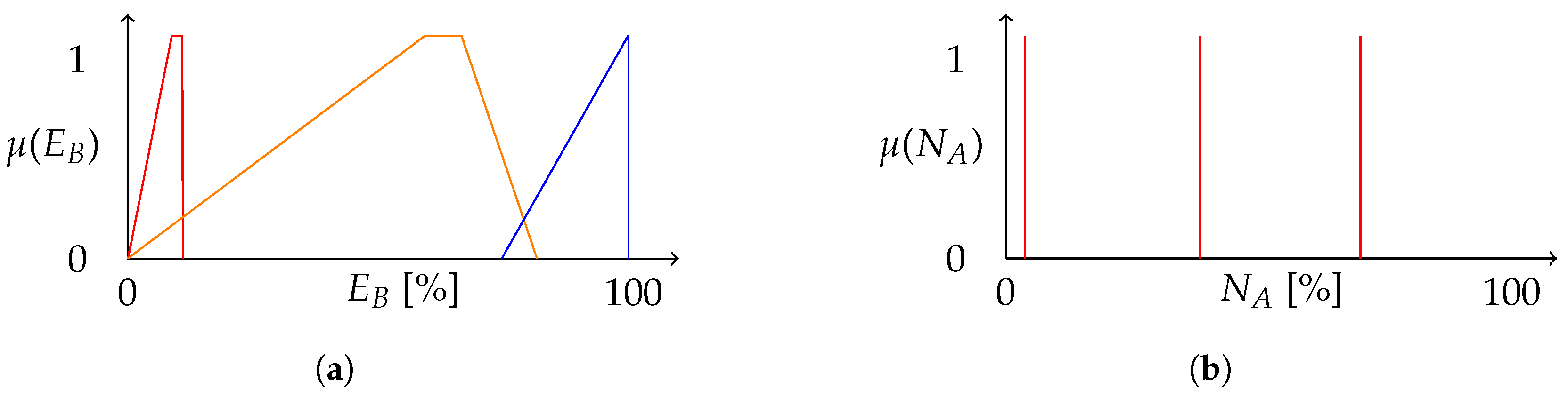
A controller was optimized for the case where no forecast was provided, and only the energy buffer’s state of charge. Three membership functions where used in this fuzzy set. The resulting input and output fuzzy sets for this controller are shown in
Figure 5.
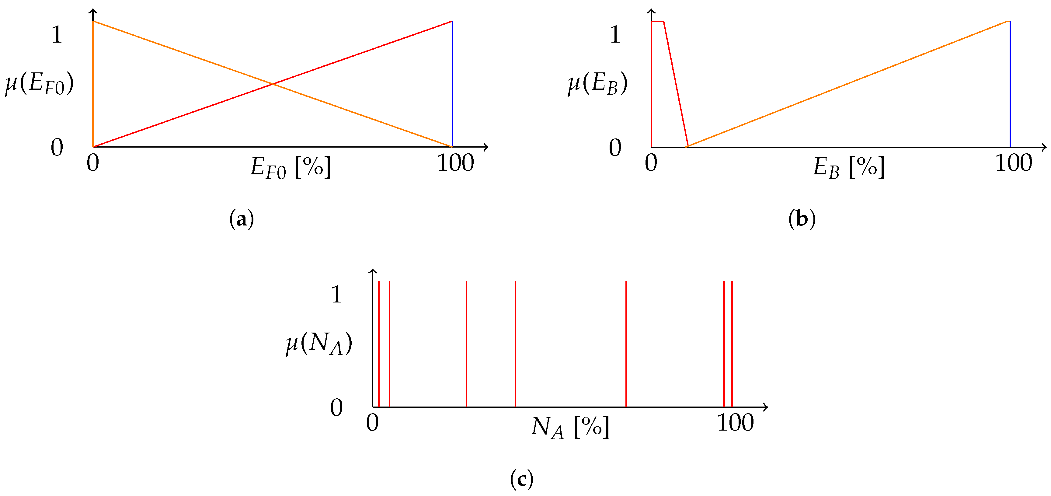
The optimization for the controller utilizing the current-day energy forecast resulted in the fuzzy sets shown in
Figure 6. In each of these inputs, one of the trapezoidal membership functions was compressed to a fuzzy singleton at 100%, overlapping with another function.
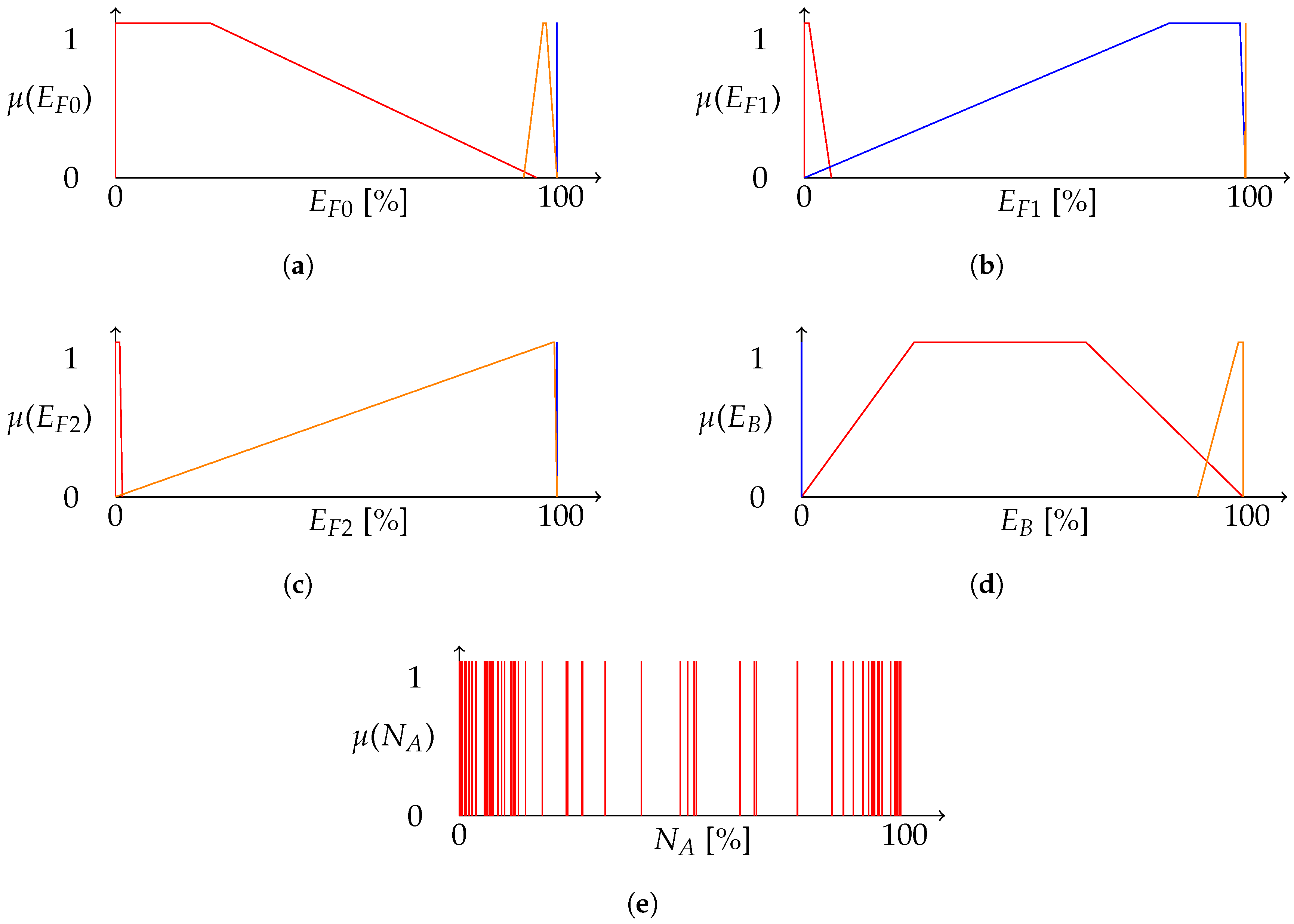
Results of the optimization where the controller was provided with current and next-day energy forecast are shown in
Figure 7. In both cases, the close proximity of singletons in the output partition may allow for reduction in the number of rules. The controller using two day forecasts optimized to a lower fitness value compared to the controller using only one day forecast (11.65 vs. 12.29).
5. Simulation Results
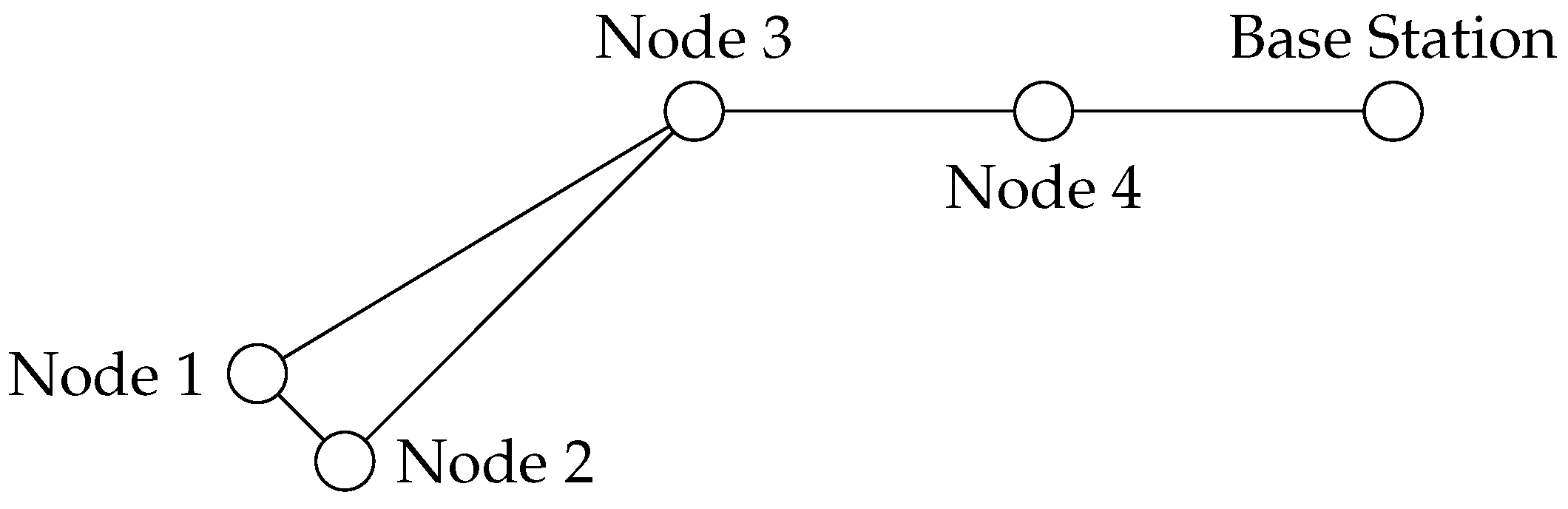
The topology of the simulated network is shown in
Figure 8. Nodes 1, 2, 3 and 4 correspond to data from the Moxee, Prosser, Lind and Garfield East stations, respectively. In this figure, the solid lines denote communication channels. This layout roughly mimics the relative positions of the actual stations. For the full simulation, all 880 days of the data set were used. During simulations, node activity levels were updated at sunrises and sunsets. An initial node activity was used prior to the first update which resulted in the bulk of the energy usage for many of the best performing simulations.
Realistic parameters associated with a node’s energy harvesting and usage have been used in this simulation [
55]. Energy storage for each node is comprised of a non-rechargeable battery and a supercapacitor used as an energy buffer. Nodes use a simple store-and-forward scheme to pass messages through the network and to the base station [
58]. The flexible nature of the simulation also allows for simple changes to be made to quickly examine a variety of different configurations, including the use of different sensors.
A human-created reference controller was used for comparison with the generated controllers [
6,
54,
55]. This controller consisted of two inputs, one for the energy forecast of the upcoming day and one for the state of the energy buffer. The fuzzy partitions for these inputs had triangular membership functions, with the energy buffer functions evenly dividing the input space and the energy forecast membership functions dividing the space based on 20% quantiles. The outputs were five fuzzy singletons, equally spaced between 0 and 100%.
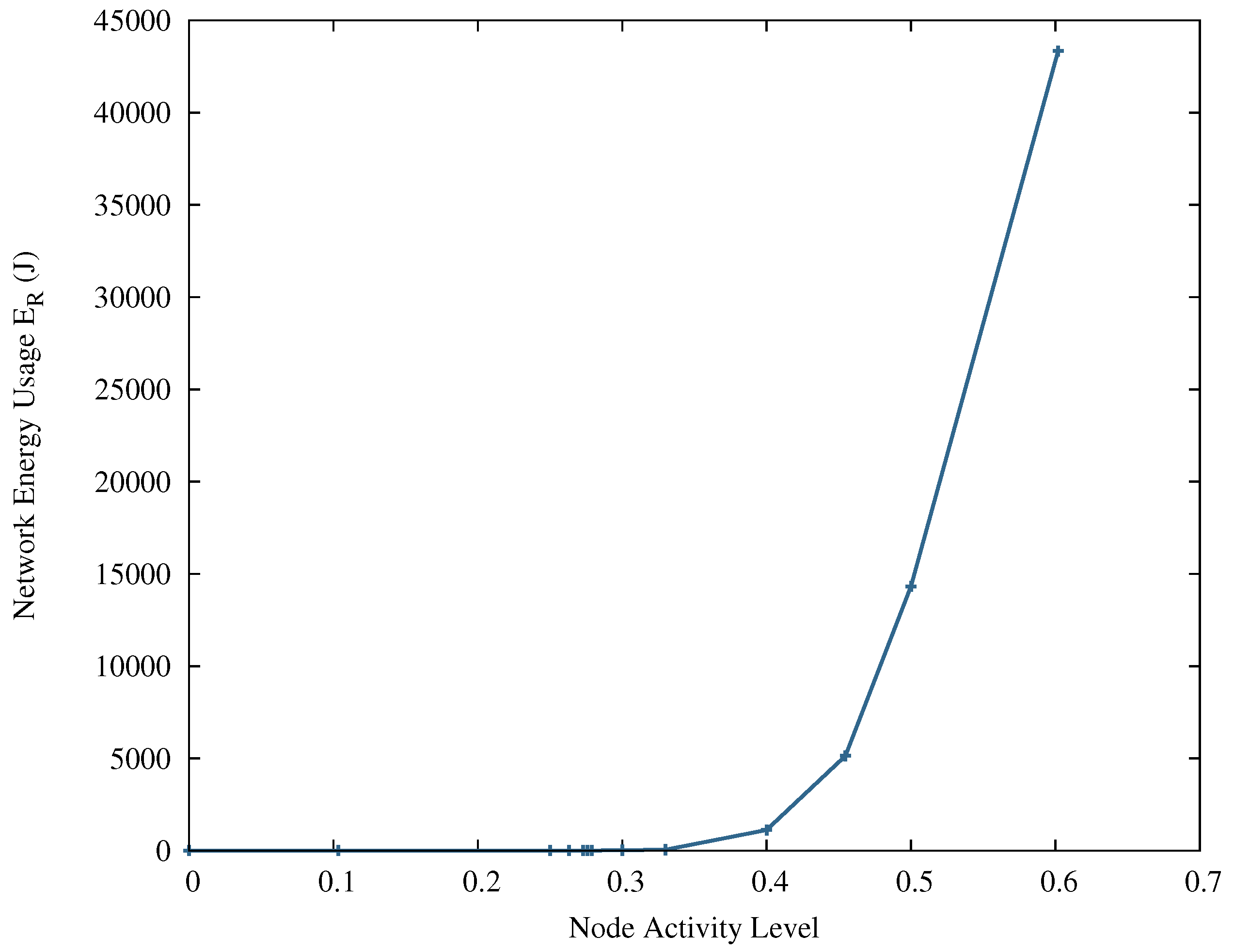
For additional comparison, simulations were performed where a constant node activity was used. A plot of energy usages for the increasing node activities is shown in
Figure 9. There was a constant amount of energy usage for simulations with node activities up to approximately 0.276, after which the amount of energy usage increased rapidly. For values of node activity above approximately 0.6, nodes began to fail due to depletion of the primary energy source. The total number of measurements taken by the network, as well as the amount of unharvested energy were both roughly linear with the increasing node activities. The linear relationship between total network measurements and the node activity allows for a regression line to be fit. The line can be described as
, where
is the total number of measurements taken during the simulation and
is the node activity.
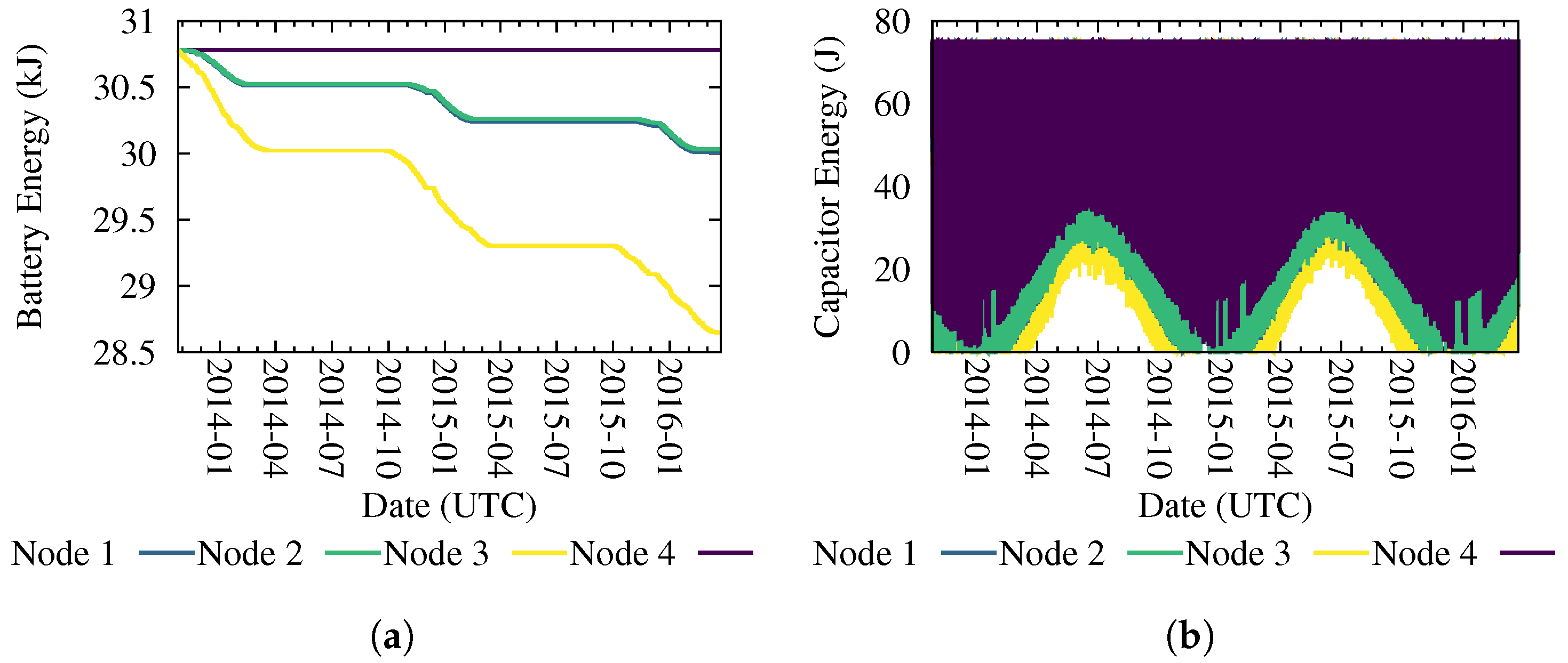
Energy values for the reference controller using a perfect energy forecast are shown in
Figure 10. The total amount of primary battery energy usage for this network during the simulation was 3646.95 J. In this simulation, the node using the largest amount of energy was Node 3, due to its central location. The node using the least amount of primary energy was Node 4, which only accepted transmissions from Node 3. The plots of supercapacitor energies in
Figure 10 support this observation, as the energy buffer for Node 4 did not drop to zero for the bulk of the simulation, while the other nodes experienced supercapacitor energy values of zero for winter months. This simulation resulted in a total of 2,391,647 measurements, with a daily minimum of 381, a daily maximum of 1162 and a daily average number of measurements of 679. Using the total number of measurements to calculate an equivalent constant node activity resulted in a value of 0.458.
Simulation results for the evolved controller using no forecast are tabulated in
Table 7. Using the total number of measurements taken, the effective activity was calculated at 0.516.
The optimized controller that used only one day of energy forecast with a perfect forecast resulted in the values shown in
Table 8. The effective activity for this controller was calculated as 0.531.
When the number of forecasts was increased to two, the simulation resulted in the values shown in
Table 9. The effective activity for this controller using a perfect forecast was calculated as 0.666.
Comparison of the simulations using the fixed values of to the reference controller shows that the human-designed controller had slightly better performance, collecting a larger number of measurements while using less energy than the equivalent constant controller. The tuned controllers improved on this performance further: they had higher equivalent constant node activities, but also used less of the total reserve energy. The no-forecast controller had a slightly lower effective activity when compared to the forecast case, but used roughly 4 times more total energy over the simulated period. The / controller uses slightly more energy while operating at a higher general activity level when compared to the controller. However, this controller demonstrates a larger variance in the number of measurements taken during a day, suggesting its greater ability to adapt to the amount of harvestable energy. The increased energy usage during this simulation is completely due to higher usage at Node 3, meaning that further improvements could be gained by allowing different nodes to employ different controllers, or through the use of an energy-aware message routing method.
When the pressure-based CART forecast is used, the summaries of the daily measurements and amounts of reserve energy usages are shown in
Table 10 and
Table 11 for the
and
/
controllers, respectively. The calculated equivalent constant node activities for these simulations were 0.520 and 0.673, respectively. Comparing these equivalent values to the values from the perfect forecast case showed a slight decrease in the case of the
controller, and an increase in the case of the
/
controller. Comparing these values to the no-forecast version, the evolved
controller had similar effective activity while still using less energy. The
/
controller still had a higher effective activity level, but at the cost of roughly 135% of the total energy usage compared to the no-forecast simulation. The increases in energy usage for the controllers utilizing a forecast arose from the errors in the generated forecast that was used as an input. The
/
controller suffered a larger increase due to the higher error associated with the forecast for the second day.
In this simulation, network energy usage climbs very quickly as the network activity level climbs past a certain point, as previously shown in
Figure 9. The
/
controller operated at a higher node activity level, which resulted in a higher energy use. When forecast errors were introduced, they took a greater toll on the energy usage for this controller because of where its usual operating point was located.
In all these cases, the tuned controllers performed better than the reference controller, with all combinations of controllers and forecasts taking more measurements while using less reserve energy during the simulation. Using perfect forecasts, the / controller had a greater equivalent node activity with a modest increase in reserve energy usage when compared to the controller, indicating a better utilization of harvestable energy. Both controllers utilizing the energy forecasts had higher activity levels and lower energy reserve usages compared to the no-forecast controller when using a perfect forecast. Comparing the differences between the perfect and pressure-based forecasts for the controller, there was an increase in reserve energy usage and a slight decrease in equivalent node activity, underscoring the importance of accurate forecasting values. For the case where two days of energy forecast were used, the controller showed a greater jump in usage of the energy reserve when comparing the perfect and pressure-based forecasts. Compared to the no-forecast controller, in this case, the / controller used more reserve energy while operating at a greater activity level.
6. Conclusions and Future Work
This contribution describes a new energy management scheme for wireless sensor nodes with solar energy harvesting capability. While energy harvesting allows nodes to replenish reserves in the field, consumption of the collected energy should be managed for its most effective usage. Estimates of energy available in the future can be used to inform rates of consumption. To that end, in this work, predictions of daily solar energies are based on hourly measurements of atmospheric pressure. These predictions are used in combination with a fuzzy logic controller to improve the usage of energy harvested by a sensor node. The membership functions of the fuzzy logic controller have been tuned using differential evolution to further improve energy utilization.
With respect to the energy forecast, the resulting forecasts using machine learning techniques provide comparable results to the estimates based on the minimum and maximum measured daily temperatures when MAPE is considered, but some methods have lower values of RMSE.
In comparison to forecasts based on minimum and maximum measured daily temperatures, the proposed machine learning forecasting techniques provide better accuracy in terms of RMSE and comparable results when MAPE is considered. The methods explored here have the additional benefits of the ease of implementation on the limited hardware that is available in sensor nodes, and a predictor variable that is easier to measure.
The controllers tuned with differential evolution outperformed the human-created reference controller, even when the perfect energy forecast was replaced with a simple solar energy forecast based on measurements of atmospheric pressure. The controller performed better than the no-forecast controller for both the perfect and generated forecasts, while the / controller saw an increases in both network activity and energy usage with respect to the no-forecast case while using the generated forecast. However, the / controllers higher network activity and larger variance in number of daily measurements with relatively modest increases in energy usage points to its more effective use of harvested energy. The relative weighting of the reserve and harvested energy values used to evaluate the potential controllers can be changed to reflect the requirements of a given application.
There are a number of possible avenues for future work. With respect to possible improvement of the simulation, a number of additional factors could be included, such as the effects of temperature, self discharge, and finite data storage capacity. An additional layer of complexity can also be included to more closely reflect deployment conditions such as occlusion of solar panels due to seasonal vegetation. These more complex facets, when added to a simulation, remain easily repeatable. The energy management scheme can be improved by increasing the frequency of activity level updates, to better follow the amount of energy present in the buffer. In addition, splitting the transmission and measurement scaling values can be considered, as these can have very different associated energy costs. Inclusion of more nodes in the simulated network will allow for the addition of the network level energy management schemes, such as energy-aware message routing and dynamic cluster head selection.


