A Comparison Study between Two MPPT Control Methods for a Large Variable-Speed Wind Turbine under Different Wind Speed Characteristics

Abstract

Variable speed wind turbines (VSWTs) usually adopt a maximum power point tracking (MPPT) method to optimize energy capture performance. Nevertheless, obtained performance offered by different MPPT methods may be affected by the impact of wind turbine (WT)’s inertia and wind speed characteristics and it needs to be clarified. In this paper, the tip speed ratio (TSR) and optimal torque (OT) methods are investigated in terms of their performance under different wind speed characteristics on a 1.5 MW wind turbine model. To this end, the TSR control method based on an effective wind speed estimator and the OT control method are firstly presented. Then, their performance is investigated and compared through simulation test results under different wind speeds using Bladed software. Comparison results show that the TSR control method can capture slightly more wind energy at the cost of high component loads than the other one under all wind conditions. Furthermore, it is found that both control methods present similar trends of power reduction that is relevant to mean wind speed and turbulence intensity. From the obtained results, we demonstrate that, to further improve MPPT capability of large VSWTs, other advanced control methods using wind speed prediction information need to be addressed.

1. Introduction

Driven by the increasing concern for environment pollution caused by traditional energy sources, electrical power generation based on renewable energy has rapidly developed during past years. As the rapidest developing renewable energy, the development of wind power generation has been impressive in recent years. According to the latest statistical data from Global Wind Energy Council [1], the global cumulative capacity of wind power has reached 486.7 GW in 2016, with a newly added capacity of 54.6 GW in 2016. It is anticipated that, in the America of 2030, more than 20% energy production will be provided by wind energy [2]. Meanwhile, Chinese government makes an energy plan [3] that non-fossil energy will rise to 15% and 20% in the national total primary energy consumption by 2020 and 2030, respectively. It is obvious that wind energy has become an important portion of energy. To further enhance its competitiveness, it is urgent to reduce the cost of wind power generation through utilizing modern technologies.

To ensure high performance while minimizing costs, optimal solutions have been developed constantly [4]. On the one side, wind turbines (WTs) have grown considerably in size over the last several years; on the other side, advanced control algorithms have been intensively studied, among which maximum power-point tracking (MPPT) method gains the most attention [5,6,7,8,9,10,11,12,13,14,15,16,17,18,19,20,21,22,23,24,25,26,27,28]. The MPPT algorithm that is used to bring the turbine to the MPP over a full wind speed range aims to maximize the efficiency of a wind turbine (WT).

In a recent study [8], MPPT algorithms were categorized into direct power controllers (DPC) and indirect power controllers (IPC). The former directly maximizes the output electrical power, while the latter maximizes the captured mechanical wind power. The DPC, which mainly refers to hill climbing search (HCS) [9], does not require WT knowledge and tracks the MPP by analyzing the power variation based on a pre-obtained system curve. However, it always takes a long time to converge. Moreover, its robust performance may not be guaranteed, for instance, when there is an oscillation around the MPP. Under the IPC, there are three types of MPPT algorithms: power signal feedback (PSF) [10], optimal torque (OT) algorithm [11] and the tip-speed ratio (TSR) algorithm [12]. The TSR algorithm depends on precise wind speed information that is hardly obtained in conventional WTs. Therefore, as alternative methods, the PSF and OT algorithms were developed and commonly used in current commercial WTs.

Principles of the PSF and OT algorithms are essentially the same and only differ in their implementation [13]: the former calculates the optimum power based on a generator speed–power table enquiry method, whereas the latter produces the optimum torque based on a conventional control unit. Since there are only several points predefined in a generator speed–power table, the PSF algorithm may be slightly inferior to the OT algorithm. However, the OT algorithm is not optimal for exploiting energy production of a large-scale WT with a large inertia. To enhance the MPPT performance, improved techniques have been proposed, such as adding a feed-forward term to assist in acceleration or deceleration [14], adopting estimation control methods to determine the accurate gain parameter [15,16] or readjusting the torque gain to match wind speed characteristics [17,18]. Nevertheless, as an alternative method, the OT algorithm is internally less accurate than the direct TSR method [8]. Therefore, to maximize power extraction, the direct TSR method is necessary to be investigated.

As the development of technology, there are now two possible TSR methods: one is to use wind information measured by an advanced sensing device, such as lidar [19,20,21], whereas the other is to use the estimated wind speed [22,23,24,25,26]. Compared to the one based on measurement devices, the estimated wind-based TSR method almost requires no additional cost and therefore receives intense attention in recent years. A typical estimated wind-based TSR method consists of two parts: an effective wind speed estimator that provides an optimal speed reference and a speed controller that tracks the speed reference. Various wind speed estimation and speed tracking algorithms have been proposed in previous studies. Nevertheless, the previous studies mainly focused on algorithm development and overlooked the impact of WT’s inertia and wind speed characteristics on obtained performance. In a study conducted by Tang et al. [27], it was shown that the power production performance of WTs under the OT algorithm was affected by both the turbine parameters and the wind speed characteristics. The study was only validated by simulation results on a 400 W WT, but the obtained result has been useful for optimizing the torque gain of the OT algorithm [17,18,28]. In this regard, an investigation on performance of the estimated wind-based TSR method under different wind speed characteristics would be helpful to understand the capability and limitation of the control method, thus potential optimization rules for MPPT method can be sorted out.

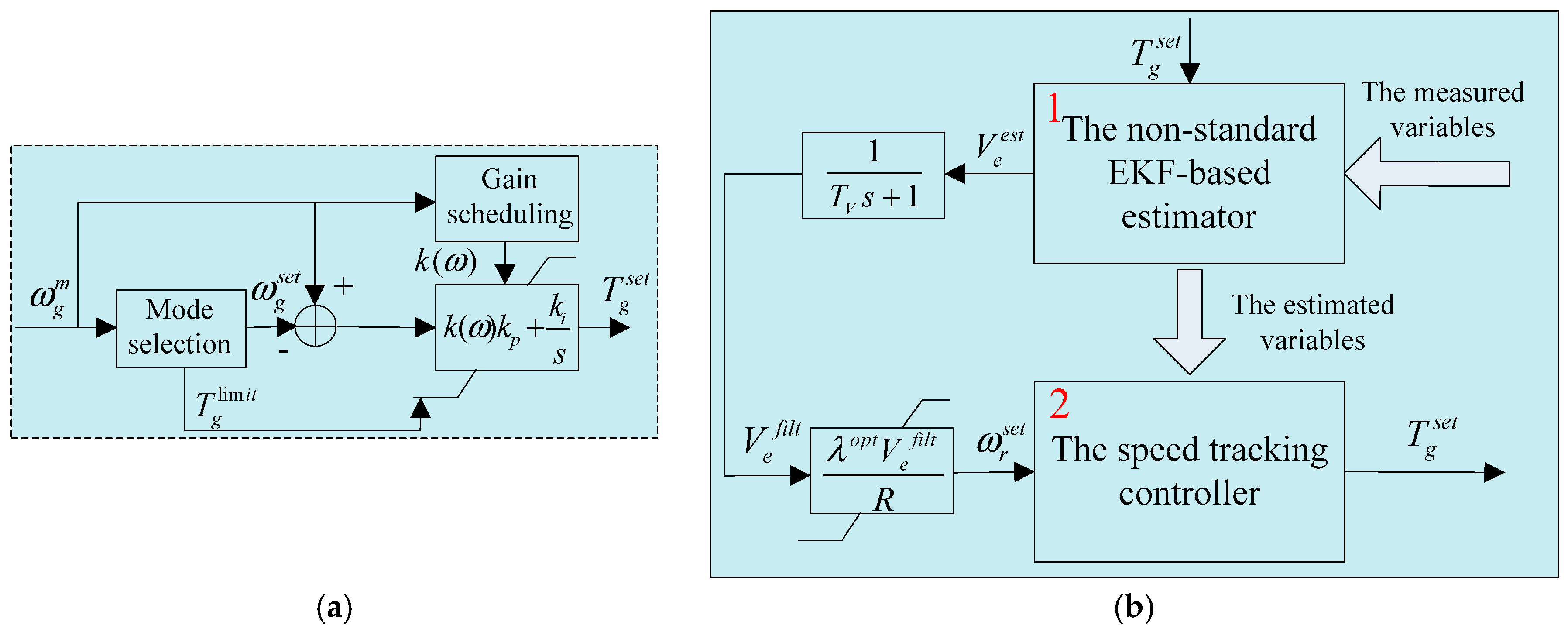
Motivated by the aforementioned observations, this paper carries out a comparison study on performance of an estimated wind-based TSR method and the OT method. The estimated wind-based TSR method tracks an optimal speed reference calculated by estimated variables from the non-standard extended Kalman filter (EKF) based wind estimation algorithm proposed in [26], whereas the OT method adopts the standard PI-based one discussed in [13]. Finally, the similarities and differences between the two methods under different wind speed characteristics are illustrated by some simulations. In addition, to provide a reliable result, a 1.5 MW variable speed WT manufactured by CMYWP (China Ming Yang Wind Power, Zhongshan, China) is used as the modeling subject and the industry-standard software for WT performance and load calculations, Garrad Hassan’s Bladed [29,30], is used to carry out simulations. Meanwhile, turbulent winds are employed to give different wind speed characteristics, thus the obtained results can be reliable and understandable.

The remainder of this work is organized as follows. The relevant WT and its modeling are introduced in Section 2. Section 3 describes the PI-based OT and the estimated wind-based TSR methods. This is followed by simulation tests and results discussions in Section 4. Finally, conclusions are drawn in Section 5.

2. The Concerned WT and Its Modeling

2.1. The Concerned WT

2.1.1. WT Basic Information

The concerned WT is a three-blade 1.5 MW doubly-fed machine with 82 m rotor diameter manufactured by the CMYWP. The WT’s specifications are shown in

Table 1. Specifications of the concerned WT.

Parameter	Value
Rotor diameters	82 m
Number of rotor blades	3
Rated electrical power	1500 kW
Rated wind speed	$10.8\mathrm{m}/\mathrm{s}$
Nominal rotor speed	$1.824\mathrm{rad}/\mathrm{s}$
Optimal TSR	9.5
Rotor moment of inertia	$4.94\times {10}^6 {\mathrm{kgm}}^2$
Generator moment of inertia	$92 {\mathrm{kgm}}^2$
Gearbox ratio	100.48
Drive train stiffness coefficient	$1.38\times {10}^8 \mathrm{Nm}/\mathrm{rad}$.
Drive train damping coefficient	$1.0\times {10}^4 \mathrm{Nms}/\mathrm{rad}$

.

The WT is a variable-speed machine with a doubly-fed induction generator (DFIG) [31,32]. As shown in Figure 1, its energy conversion system diagram includes a blade rotor, a high-ratio gearbox, a DFIG and a partial scale power converter.

2.1.2. The WT’s Characteristic Curves

By using the Bladed software, the characteristic curves of the WT are obtained. Curves of the aerodynamic power coefficient (C_p) corresponding to different TSR ($\lambda$) and pitch angle ($\beta$) are shown in Figure 2. It is known from Figure 2 that, for the concerned WT, the maximum $C_p^{max}$ is 0.483, the corresponding optimal $\beta$ and optimal $\lambda$ are 0° and 9.5, respectively. Therefore, to maximize wind energy capture, the method for the WT is to maintain its pitch angle at 0° and its TSR at 9.5.

2.2. The WT Modeling

In this paper, the WT model includes a drive train system and the blade rotor aerodynamics.

The drive train is described by two inertias interconnected by a spring and a damper. The external forces to this 2 degree of freedom (DOF) system are the aerodynamic torque on the slow speed shaft and the generator reaction torque on the high speed shaft. The governing motion equation of this model is given by:

$$\begin{array}{l}{J}_g{\dot{\omega }}_g=T_{sh}/N-T_g\\ J_r{\dot{\omega }}_r=T_a-T_{sh}\\ T_{sh}=s_{dt}\gamma +d_{dt}\dot{\gamma }\end{array}$$

(1)

where $\gamma =({\theta }_r-{\theta }_g/N)$; ${\omega }_r$ and ${\omega }_g$ are rotor and generator rotational speeds, respectively; ${\theta }_r$ and ${\theta }_g$ are rotor and generator rotational angles, respectively; $s_{dt}$ and $d_{dt}$ are stiffness and damping coefficients of drive train, respectively; $J_r$ and $J_g$ are inertias of blade rotor and generator, respectively; $T_a$ and $T_g$ are aerodynamic torque and generator torque, respectively; and $N$ is gearbox ratio.

The model of the aerodynamic power $P_a$ is expressed as:

$$P_a=T_a{\omega }_r=\rho \pi R^2{V}^3{C}_p(\lambda ,\beta )/2=\rho \pi {\omega }_r{R}^3{V}^2{C}_q(\lambda ,\beta )/2$$

(2)

where $\rho$ is air density, $R$ is rotor radius, $V$ is the effective wind speed, and $C_p(\lambda ,\beta )$ is aerodynamic power coefficient which is a nonlinear function of the TSR ($\lambda$) and pitch angle ($\beta$). The $\lambda$ is defined by:

$$\lambda ={\omega }_{r}R/V$$

(3)

3. The Two MPPT Methods

In this section, the two MPPT methods are presented and analyzed. Since the OT control method is now a standard method used in commercial WT control systems, only a short description will be given. The estimated wind-based TSR method is not standard, so this method will be elaborated in detail. The structures of the OT-based controller and the TSR-based controller with a wind speed estimator are shown in Figure 3a,b, respectively. These two controllers are explained as follows.

3.1. The Standard OT-Based Controller

As shown in Figure 3a, the OT-based controller consists of a PI unit, a gain scheduling unit and a mode selection unit. Because its design has been addressed in previous studies [13], for the sake of simplicity, only their implementations are shortly described here.

The PI unit can be formulated as:

$$T_g^{set}=(k(\omega )k_p+k_i/s)({\omega }_g^m-{\omega }_g^{set})$$

(4)

where $T_g^{set}\in [T_g^{\min },T_g^{\max }]$ and ${\omega }_g^{set}$ are the torque set-point and speed reference, respectively; the $k_p$ and $k_i$ are the proportional and integral gains, respectively; ${\omega }_g^m$ is the measured generator speed; and $k(\omega )$ is the scheduled gain.

The gain scheduling unit calculates $k(\omega )$ that is used to compensate the variation of the aerodynamic sensitivity [29]. Besides, the mode selection unit determines speed reference ${\omega }_g^{set}$ and the torque limitations $T_g^{\min }$ and $T_g^{\max }$ for the PI unit. The control rule of the mode selection unit is summarized in

Table 2. Control rule of the mode selection unit.

Condition	${\mathit{\omega }}_{\mathit{g}}^{\mathit{s}\mathit{e}\mathit{t}}$	${\mathit{T}}_{\mathit{g}}^{\mathbf{min}}$	${\mathit{T}}_{\mathit{g}}^{\mathbf{max}}$
${\omega }_g^m<({\omega }_g^{cutin}+{\omega }_g^{rated})/2$	${\omega }_g^{cut\mathrm{in}}$	0	$T_g^{opt}$
${\omega }_g^m\ge ({\omega }_g^{cutin}+{\omega }_g^{rated})/2$	${\omega }_g^{rated}$	$T_g^{opt}$	$T_g^{rated}$

.

In Table 2, ${\omega }_g^{cut\mathrm{in}}$ and ${\omega }_g^{rated}$ are the cut-in and rated generator speeds, respectively; and $T_g^{opt}$ is the optimal generator torque and given by:

$$T_g^{opt}=K^{opt}{({\omega }_g^m)}^2$$

(5)

where $K^{opt}$ is the optimal gain and calculated by:

$$K^{opt}=(1/2)\rho \pi R^5{C}_p^{\max }/{({\lambda }^{opt}N)}^3$$

(6)

3.2. The Estimated Wind-Based TSR Controller

As shown in Figure 3b, the estimated wind-based TSR controller mainly consists of a wind speed estimator and a speed tracking controller. In this section, these two parts will be elaborated as follows.

3.2.1. The Speed Tracking Controller

To design the speed tracking controller, the WT model in Equations (1) and (2) is utilized. Provided ${\omega }_r={\omega }_g/N$, Equation (1) is simplified as:

$$J_R{\dot{\omega }}_r=T_a-N{T}_g$$

(7)

where $J_R=J_r+N^2{J}_g$.

To obtain an explicit relation between ${\omega }_r$ and ${\dot{T}}_g$, time derivative of Equation (7) is deduced as:

$$J_R{\ddot{\omega }}_r=(\partial T_a/\partial {\omega }_r){\dot{\omega }}_r+(\partial T_a/\partial V)\dot{V}+(\partial T_a/\partial \beta )\dot{\beta }-N{\dot{T}}_g$$

(8)

Since the pitch angle remains constant, Equation (8) can be further simplified as:

$$J_R{\ddot{\omega }}_r=(\partial T_a/\partial {\omega }_r){\dot{\omega }}_r+(\partial T_a/\partial V)\dot{V}-N{\dot{T}}_g$$

(9)

Now considering the rotor speed tracking problem, the final closed-loop system can be assumed as an ideal second-order dynamic system denoted by:

$${\ddot{\epsilon }}_{\omega }+2{\xi }_t{\omega }_t{\dot{\epsilon }}_{\omega }+{\omega }_t^2{\epsilon }_{\omega }=0$$

(10)

where ${\epsilon }_{\omega }={\omega }_r^{set}-{\omega }_r^m$ is the tracking error, and ${\xi }_t$ and ${\omega }_t$ are the damping factor and crossover frequency, respectively. When neglecting the dynamics of the speed set-point, Equation (10) is simplified as:

$${\ddot{\omega }}_r^m=-2{\xi }_t{\omega }_t{\dot{\omega }}_r^m+{\omega }_t^2({\omega }_r^{set}-{\omega }_r^m)$$

(11)

By integrating Equations (9) and (11), with ${\omega }_r={\omega }_r^m$, the control action ${\dot{T}}_g$ can be derived as:

$${\dot{T}}_g=J_R[2{\xi }_t{\omega }_t{\dot{\omega }}_r-{\omega }_t^2({\omega }_r^{set}-{\omega }_r)]/N+[(\partial T_a/\partial {\omega }_r){\dot{\omega }}_r+(\partial T_a/\partial V)\dot{V}]/N$$

(12)

From Equation (12), it is obvious that ${\dot{T}}_g$ is determined by the rotor speed set-point ${\omega }_r^{set}$. To obtain the ${\omega }_r^{set}$, the wind speed has to be estimated. Besides, some other dynamics: $\partial T_a/\partial {\omega }_r$, $\partial T_a/\partial V$, $\dot{V}$ and ${\dot{\omega }}_r$ also need to be obtained. In this study, these variables are estimated by a non-standard EKF-based wind speed estimator.

3.2.2. Non-Standard EKF-Based Wind Speed Estimator

To design an EFK-based estimator, the concerned system has to be modeled in the following nonlinear form [33,34]:

$$\begin{array}{l}\dot{x}=f(x,u)+w\\ y=h(x,u)+v\end{array}$$

(13)

where $x$, $u$ and $y$ are state, input and measurement, respectively; $f(x,u)$ and $h(x,u)$ are state transition function and output function, respectively; and $w$ and $v$ are the process noise and the measurement noise, respectively.

According to [26], the non-standard EKF-based solution requires at least three modeling parts: the effective wind speed, aerodynamic power and drive train. Regarding the actual need of Equation (12), these three parts are modeled and given as follows.

$$\begin{array}{l}\dot{V}=V_1+w_V\\ {\dot{V}}_1=V_2+w_{V1}\\ {\dot{V}}_2=-N_b^2{\omega }_r^2{V}_1-2N_b{d}_v{\omega }_r{V}_2+w_{V2}\end{array}$$

(14a)

$${\dot{P}}_a=(\partial P_a/\partial {\omega }_r)a_r+(\partial P_a/\partial \beta ){\beta }_1+(\partial P_a/\partial V)V_1+w_{Pa}$$

(14b)

$$\begin{array}{l}{\dot{\omega }}_r=a_r+w_{\omega r}\\ {\dot{a}}_r=[{\dot{T}}_a-s_{dt}({\omega }_r-{\omega }_g/N)-d_{dt}(a_r-a_g/N)]/J_r+w_{ar}\\ {\dot{\omega }}_g=a_g+w_{\omega g}\\ {\dot{a}}_g=[s_{dt}({\omega }_r-{\omega }_g/N)/N+d_{dt}(a_r-a_g/N)/N-{\dot{T}}_g]/J_g+w_{ag}\end{array}$$

(14c)

where $V$ is the estimated effective wind speed; $V_1$ and $V_2$ are the derivative and the second derivative of $V$, respectively; $N_b$ and $d_V$ are blade number and damping factor, respectively; $w_V$, $w_{V1}$ and $w_{V2}$ are the process noises of $V$, $V_1$ and $V_2$, respectively; $a_r$ and $a_g$ are acceleration speeds of rotor and generator, respectively; $w_{\omega r}$, $w_{ar}$, $w_{\omega g}$ and $w_{ag}$ are the process noises of ${\omega }_r$, $a_r$, ${\omega }_g$ and $a_g$, respectively; and $w_{Pa}$ is the process noise of $P_a$.

Besides, the measurement part is also required. For the non-standard EKF-based wind speed estimator, the virtual wind speed measurement is derived by:

$$V^m={(2P_a/(\rho \pi R^2{C}_p(\lambda ,\beta )))}^{1/3}+v_V$$

(15a)

where $v_V$ is the measurement noise of $V$.

The aerodynamic power measurement is given by:

$$P_a^m=P_e^m+(J_r{a}_r^m+N{J}_g{a}_g^m){\omega }_r^m+v_{pa}$$

(15b)

where $v_{Pa}$ is the measurement noise of $P_a$.

Other measurements are given by:

$${\omega }_r^m={\omega }_r+v_{\omega r}$$

(15c)

$$a_r^m=a_r+v_{ar}$$

(15d)

$${\omega }_g^m={\omega }_g+v_{\omega g}$$

(15e)

$$a_g^m=a_g+v_{ag}$$

(15f)

where $v_{\omega r}$, $v_{ar}$, $v_{\omega g}$ and $v_{ag}$ are the measurement noises of ${\omega }_r$, $a_r$, ${\omega }_g$ and $a_g$, respectively.

By using Equations (14) and (15), the whole model is in the same form as that in Equation (13), where $x$, $u$ and $y$ are given by:

$$x={(V{V}_1{V}_2{P}_a{\omega }_r{a}_r{\omega }_g{a}_g)}^T$$

(16a)

$$u={({\dot{T}}_{g}0)}^T$$

(16b)

$$y={(V^m{P}_a^m{\omega }_r^m{a}_r^m{\omega }_g^m{a}_g^m)}^T$$

(16c)

After establishing the complete model set in the form of Equation (13), the estimator can be developed by using standard EKF algorithm. The standard EKF algorithm for a continuous-discrete nonlinear system is implemented in two steps [33,34]:

Step 1: update state estimation

$${\widehat{x}}_{k|k-1}={\widehat{x}}_{k-1}+f({\widehat{x}}_{k-1},u_{k-1},t_{k-1}))T_s$$

(17a)

$${\widehat{x}}_k={\widehat{x}}_{k|k-1}+K_k(y_k-h({\widehat{x}}_{k-1},u_k,t_k))$$

(17b)

Step 2: update filter gain

$$P_{k+1|k}={\mathrm{\Phi }}_k{P}_k{\mathrm{\Phi }}_k^T+{\mathrm{\Gamma }}_k{Q}_k{\mathrm{\Gamma }}_k^T$$

(18a)

$$K_{k+1}=P_{k+1|k}{H}_{k+1|k}^T{(H_{k+1|k}{P}_{k+1|k}{H}_{k+1|k}^T+R_{k+1})}^{-1}$$

(18b)

$$P_{k+1}=P_{k+1|k}-K_{k+1}{H}_{k+1|k}{P}_{k+1|k}$$

(18c)

where ${\mathrm{\Phi }}_k=\exp (T_s{F}_k)$, ${\mathrm{\Gamma }}_k={\mathrm{\Phi }}_k{F}_k^{-1}-F_k^{-1}$, $F_k=\partial f(x^{*},u_k,t_k)/\partial x$ and $H_k=\partial h(x^{*},u_k,t_k)/\partial x$.

4. Case Study

A comparison study between the PI-based OT method and the estimated wind-based TSR method is described in this section. In theory, the two MPPT methods are equivalent because they track the same optimal TSR. However, due to the large inertia of the WT, there exist differences between applying the OT method and the TSR method in terms of their dynamic performance. To illustrate these, five cases were investigated for the two methods. For each case, wind conditions were defined according to design load case 1.1 of IEC-standard [35].

4.1. Simulation Settings

The two MPPT controllers were developed and tested on the concerned WT model using Bladed. Simulation tests were carried out through the predefined wind speeds. During the simulation tests, the two controllers were employed under same wind conditions.

4.1.1. Wind Speed Characteristics

Based on the normal turbulent model defined in [35], wind speed characteristics was defined by the following equation:

$${\sigma }_1=I_{ref}(0.75V_{hub}+b)$$

(19)

where ${\sigma }_1$ is the turbulence standard deviation; $I_{ref}$ is the expected value of the turbulent intensity (TI) at 15 m/s; $V_{hub}$ is the hub height wind speed, and b = 5.6 m/s; and ${\sigma }_1/V_{hub}$ is the (TI).

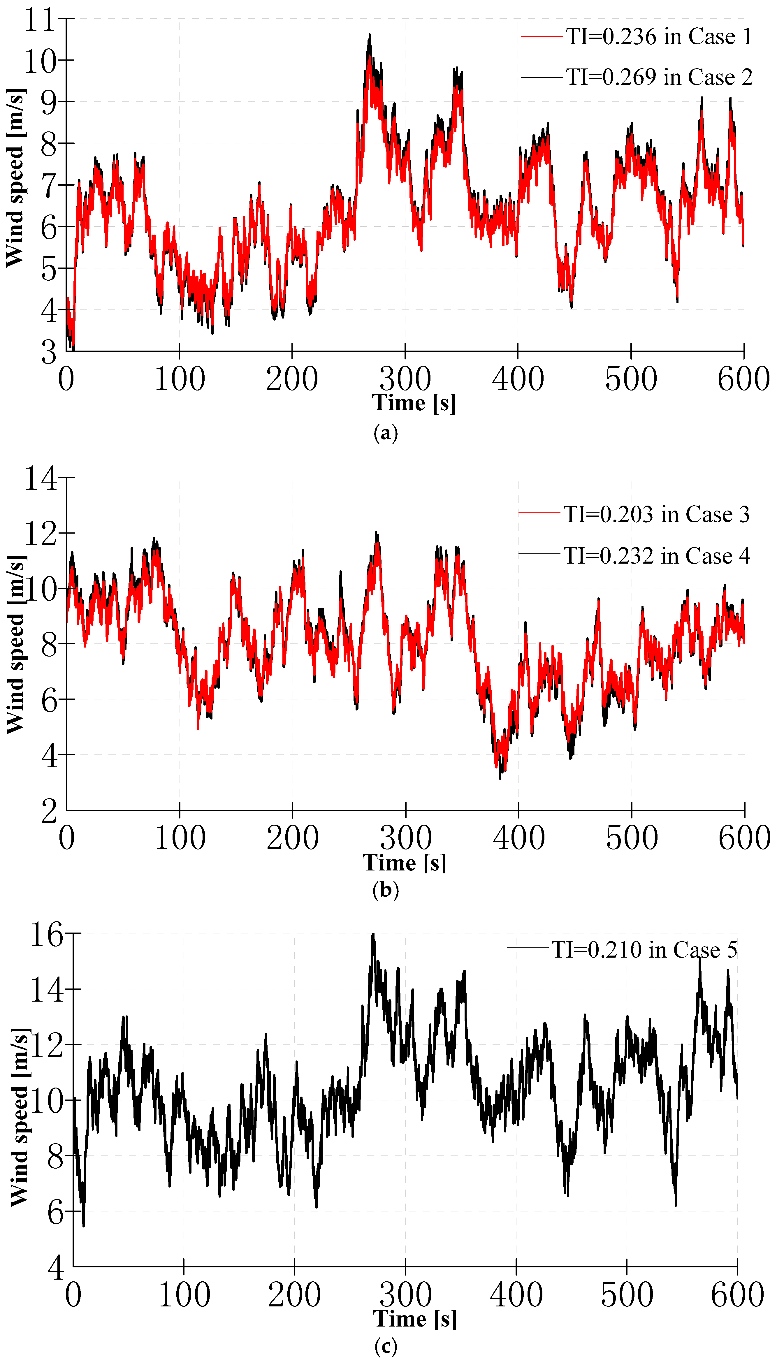
For the five simulation cases, the variables used in Equation (19) are summarized in

Table 3. Wind Speed Characteristics for Two Simulation Cases.

Simulation Case	${\mathit{V}}_{\mathit{h}\mathit{u}\mathit{b}}$	${\mathit{I}}_{\mathit{r}\mathit{e}\mathit{f}}$	${\mathit{\sigma }}_1$	TI
Case 1	6 m/s	0.14	1.414	0.236
Case 2	6 m/s	0.16	1.616	0.269
Case 3	8 m/s	0.14	1.624	0.203
Case 4	8 m/s	0.16	1.856	0.232
Case 5	10 m/s	0.16	2.096	0.210

, and the wind speed curves are shown in Figure 4.

4.1.2. Controller Parameters

For the OT controller, $K^{opt}=0.1269$; the PI gains are chosen by observation of the system response to step inputs: $k_p=88.0$ and $k_i=33.0$; and $k(\omega )=1$ because the variation of the aerodynamic sensitivity is negligible.

For the TSR controller, the damping factor and crossover frequency are selected to guarantee qualified performance for a second-order system: ${\xi }_t=0.9$ and ${\omega }_t=0.2$. The low pass filter time is set as $T_V=1.0$. For the wind speed estimator, the damping factor $d_v$ is set to 1.2. The initial state covariance ${\widehat{x}}_0$, prediction covariance $P_0$, the process variance $Q$ and measurement covariance $R$ are chosen as:

$${\widehat{x}}_0={(800P_e^m{\omega }_r^m{a}_r^m{\omega }_g^m{a}_g^m)}^T$$

(20a)

$$P_0=diag(1 \times {10}^{-1},1\times {10}^{-1},1\times {10}^{-1},1\times {10}^6,1\times {10}^{-3},1\times {10}^{-3},1\times {10}^{-2},1\times {10}^{-2})\frac{\pi }{3}$$

(20b)

$$Q=diag(1\times {10}^{-1},1\times {10}^{-2},1,1\times {10}^4,1\times {10}^{-4},1\times {10}^{-8},1\times {10}^{-2},1\times {10}^{-2})$$

(20c)

$$R=diag(1 \times {10}^{-1},1\times {10}^8,1\times {10}^{-8},1\times {10}^{-6},1\times {10}^{-6},1\times {10}^{-4})$$

(20d)

4.2. Simulation Results

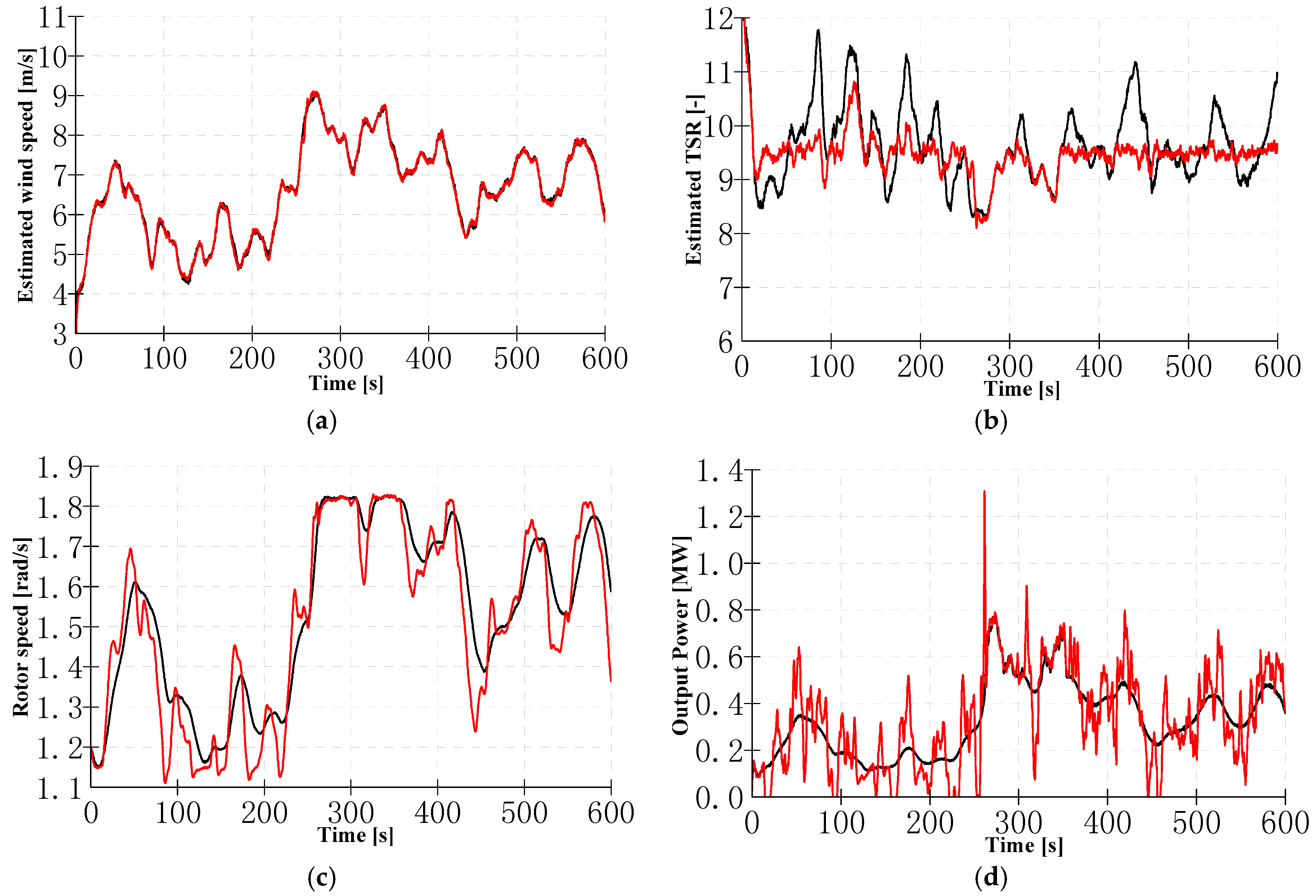
Since power production and component loads are determined by the WT operation, the rotor speed, output power, and the estimated TSR that are relevant to WT operation were measured. Meanwhile, the estimated wind speeds were also presented to check the effectiveness of the estimator. To clearly show the performance differences between the two controllers, their simulation results were together presented, where black curves and red curves are the OT controller and the TSR controller, respectively.

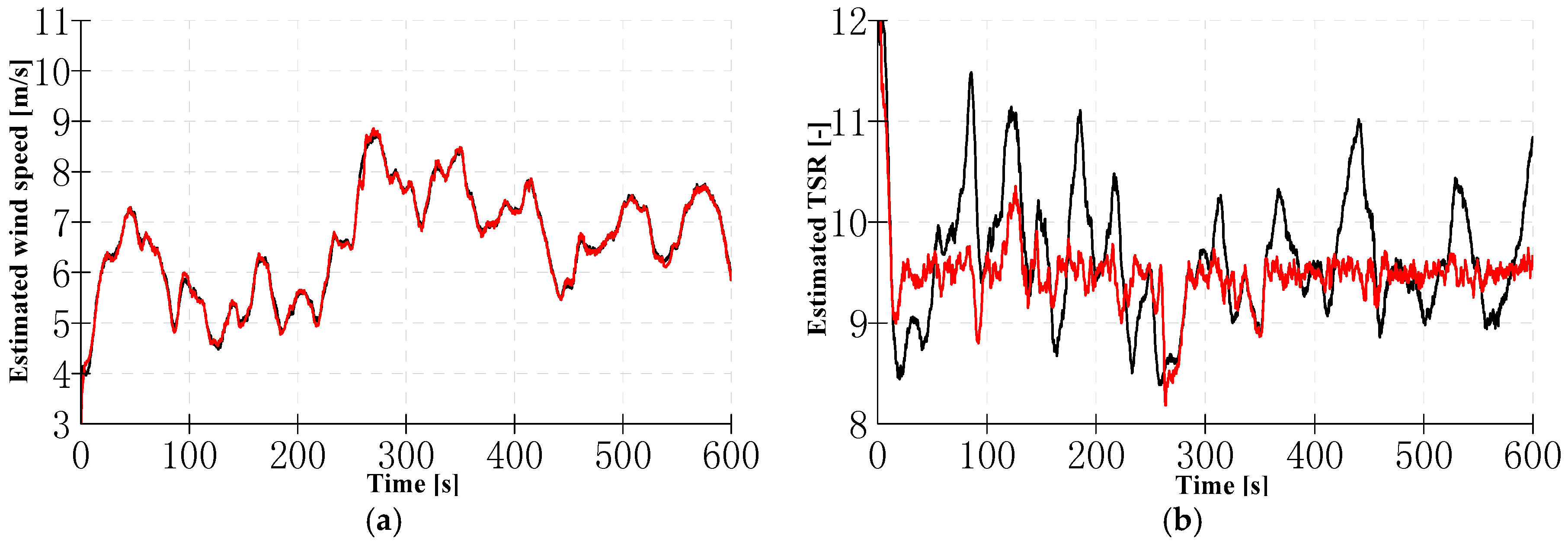
The simulation results for Cases 1 and 2 with mean wind speeds of 6 m/s and different TIs are shown in Figure 5 and Figure 6, respectively. It can be seen that, in these two cases, except the estimated winds, other three variables presented obvious differences between two controllers. The high similarities among the real wind speeds shown in Figure 4a and the estimated wind speeds shown in Figure 5a and Figure 6a justified the effectiveness of the developed estimator. The differences among curves of rotor speed, the estimated TSR and output power are summarized as follows:

• Following the variation of wind speed, the estimated TSR by the OT controller presented obvious fluctuations. By comparison, the estimated TSR by the TSR controller was maintained around the optimal value of 9.5.
• The rotor speed by the TSR controller followed the variation of wind speed, whereas the rotor speed by the OT controller gave a loose follow. Meanwhile, it can be found that the rotor speeds lagged behind the wind speeds.
• The output power by the OT controller was smooth, while the one by the other controller showed intensive variations.

When compared the results between Figure 5 and Figure 6, all curves presented high similarities, and there was only a slight difference that the curves of estimated TSR, rotor speed, and output power in Figure 6 presented slight bigger variations than the ones in Figure 5. Such a difference was induced by the increased TI.

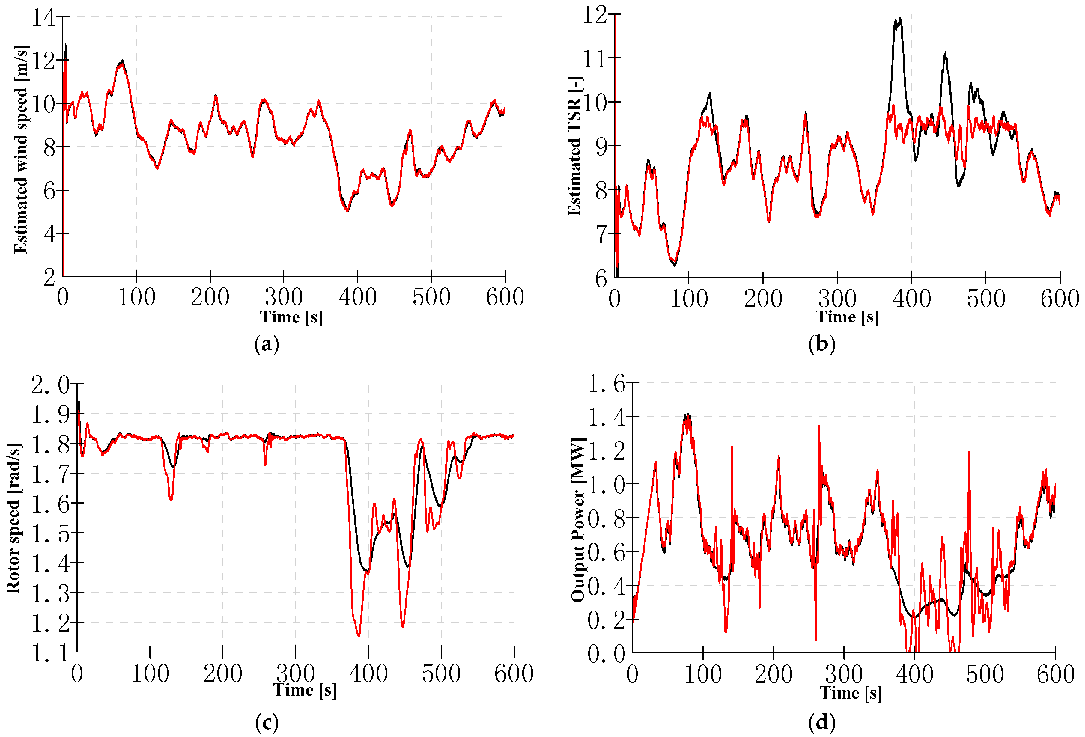
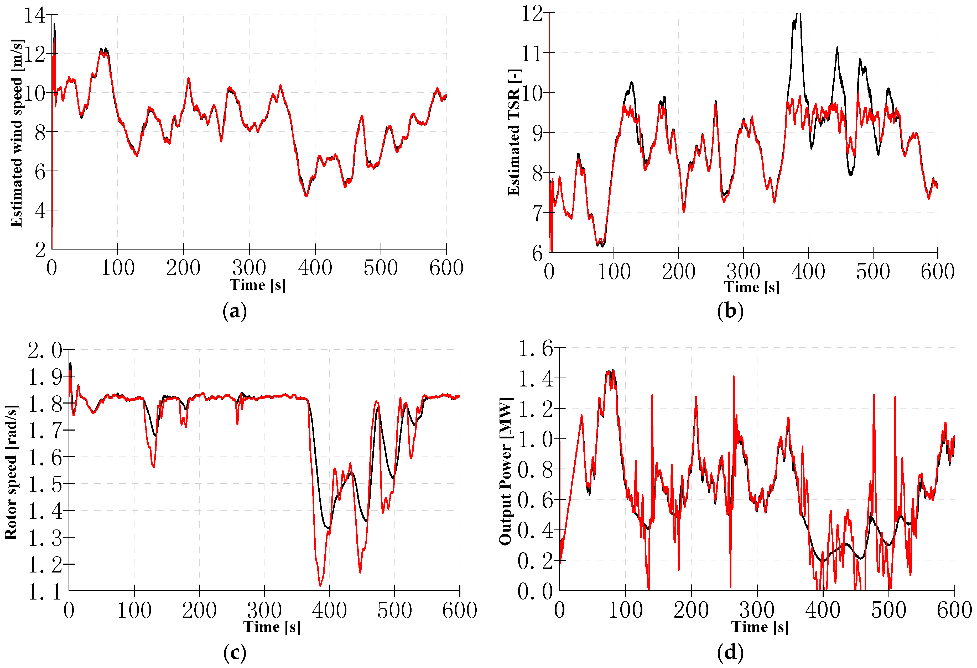
The simulation results for Cases 3 and 4 with mean wind speeds of 8 m/s and different TIs are shown in Figure 7 and Figure 8, respectively. From results in these two cases, similar trends as the ones in Cases 1 and 2 can be found: the rotor speed and output power by the TSR controller varied intensively, while the ones by the OT controller gave smooth results. Comparing to the results in Figure 5 and Figure 6, there was less difference between the estimated TSRs of two controllers. The reason is that the rotor speed reached the rated value of 1.824 rad/s when wind speeds increased up to a certain value. Under this circumstance, the two controllers were used to maintain the rated speed rather than tracking the optimal TSR.

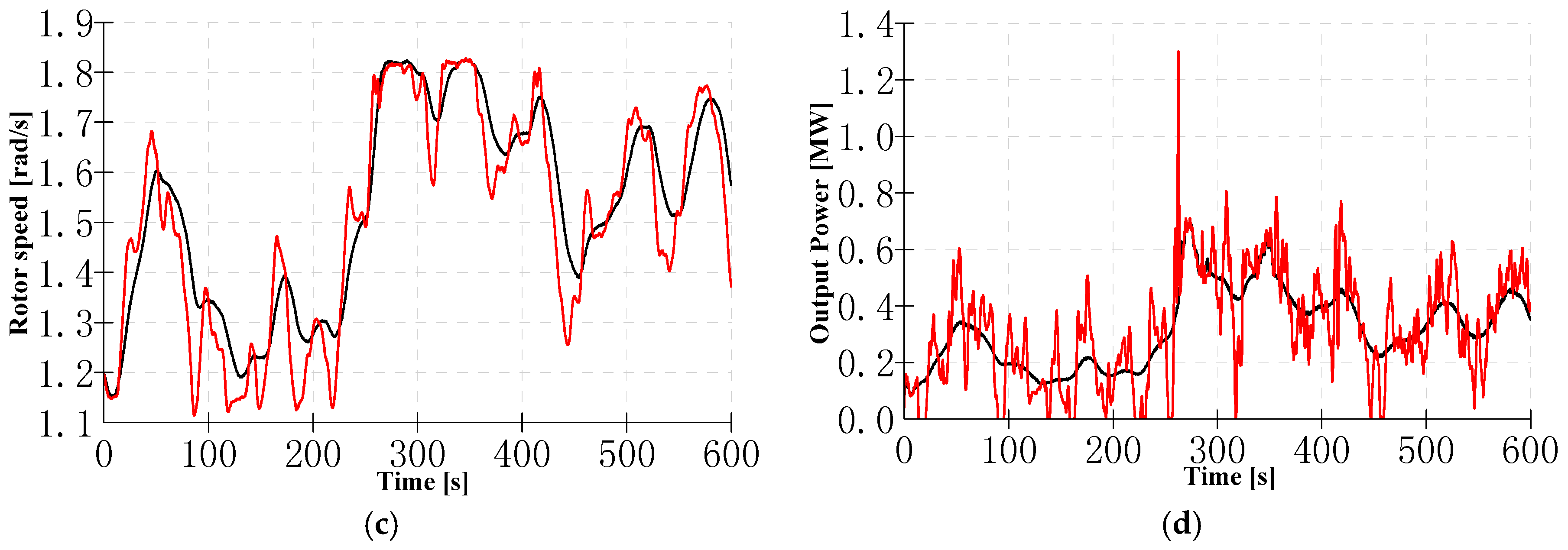
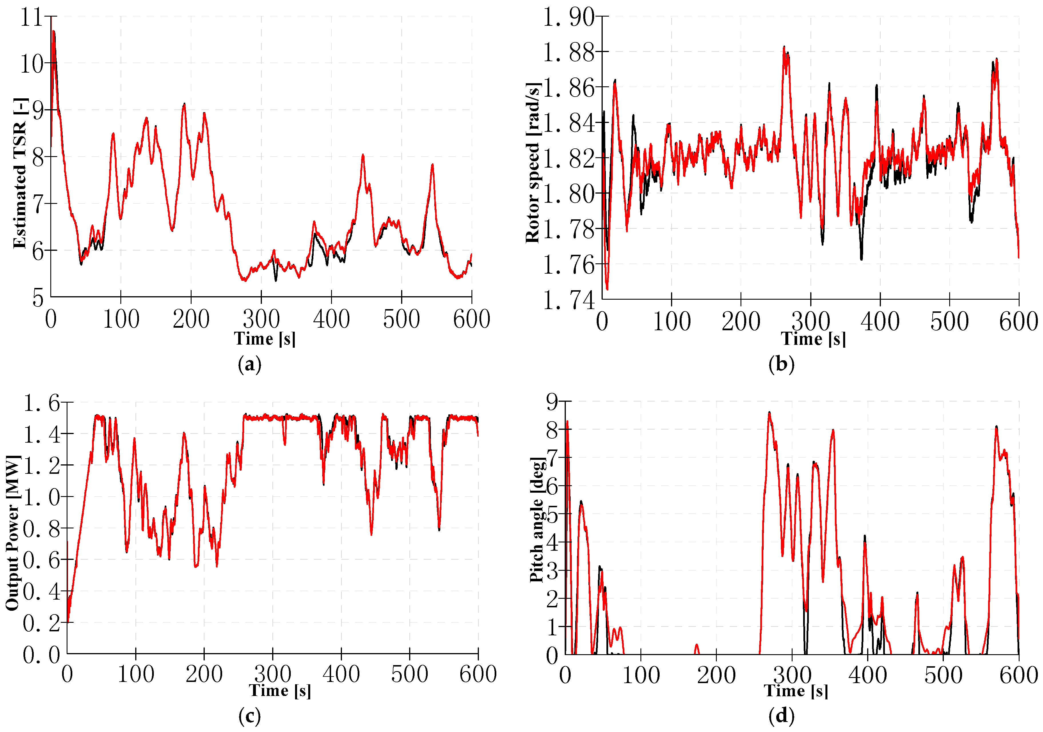
The simulation results for Case 5 with mean wind speed of 10 m/s and TI of 0.210 are shown in Figure 9. From results in this case, different trends from the ones in Cases 1–4 are found: the curves of estimated TSR, rotor speed and output power under two controllers were similar to each other. The reason is that both of the TSR and OT controllers controlled the rotor speeds around the rated value when wind speed was close to the rated wind speed of 10.8 m/s, whereas the pitch controllers were activated to maintain the rotor speed at the rated value when the wind speed was higher than its rated value. Nevertheless, there were still small differences for results of the two controllers: during the time range of 380–500 s, the rotor speed by the TSR controller was well held around the rated value and gave less variation than the one by the OT controller. Accordingly, the pitch controller operated in parallel with the TSR controller gave less pitch action than the one with the OT controller. Therefore, it can be concluded that through cooperating with the pitch controller, both of the two controllers offered a successful transition between partial and full load operation. Meanwhile, the TSR controller gave a slightly smoother transition than its counterpart.

From above observations, it can be known that the TSR controller outperformed the OT controller in terms of optimal TSR tracking, but the payback was noticeable variations of rotor speed and output power. Meanwhile, their performance was affected by the wind characteristics. Consequently, these two controllers may have different performance in terms of power production and load performance, which will be discussed in the next section.

4.3. Peformance Comparisons Based on Statistical Data

4.3.1. Power Production Comparisons

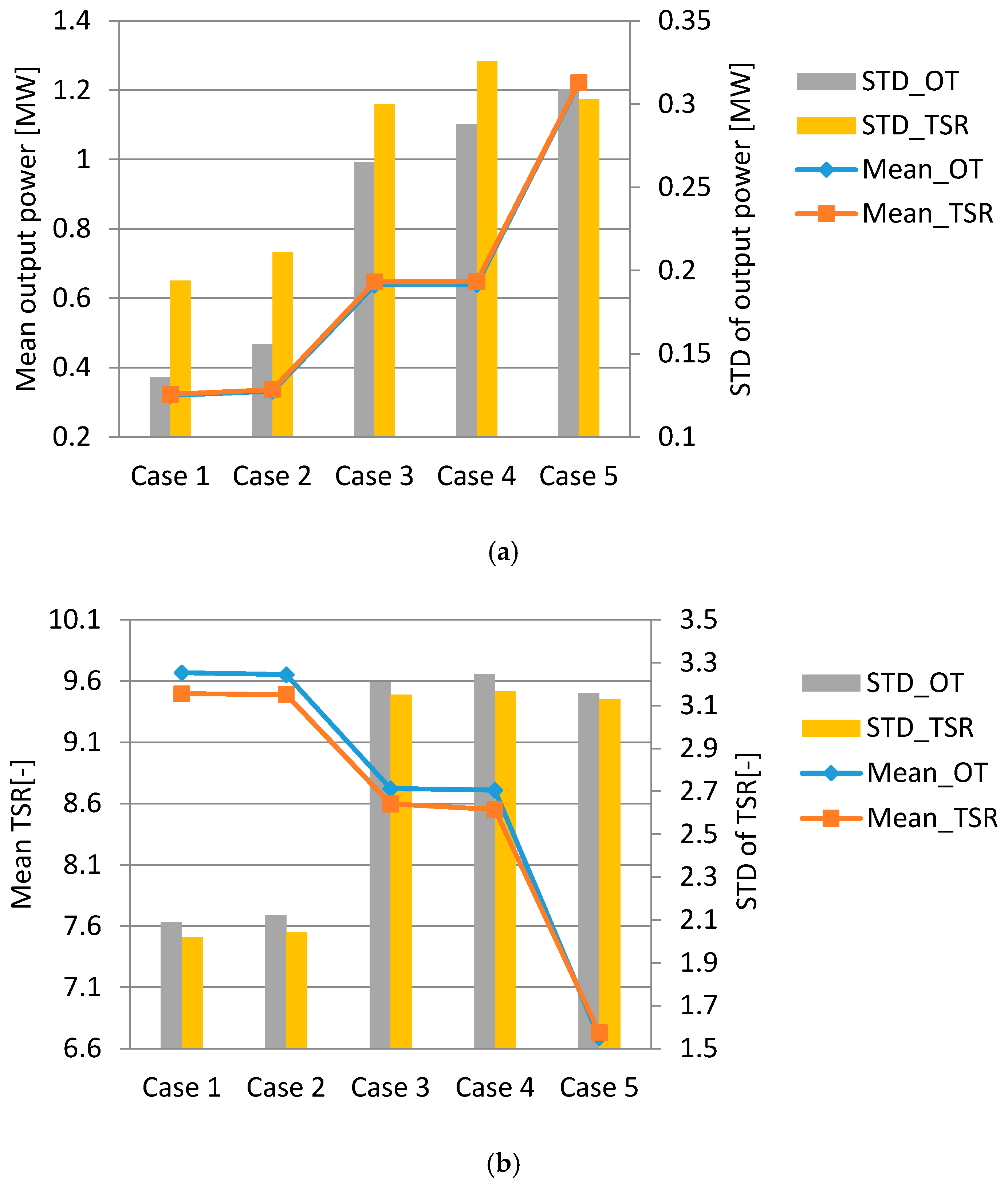
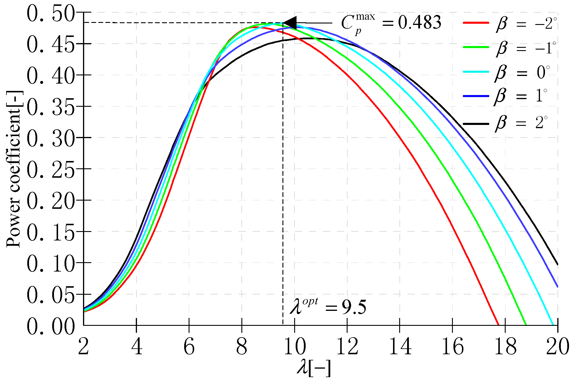
To evaluate the power production performance of the two controllers, the averaged value and the standard deviation of the output power and the TSR were calculated and compared. Figure 10a,b shows results of the output power and the TSR for the two controllers under different wind speed characteristics, respectively. The results in Figure 10a reveal the fact that both the mean value and standard deviation of the output power under the two controllers were gradually increased from Case 1 to Case 4, which means that the two controllers produced more power when the mean value or the TI of wind speed increased. At Case 5, the two controllers produced nearly same output power. To further clarify the feature of the two controllers under different wind speed characteristics, the power reduction $P_{red}$ were calculated and illustrated in

Table 4. Power reduction of two controllers under different simulation cases.

Controller	Case 1	Case 2	Case 3	Case 4	Case 5
OT controller	5.3%	4.4%	20.3%	19.2%	21.9%
TSR controller	1.8%	0.6%	20.1%	19.1%	21.8%

. The power reduction was calculated by:

$$P_{red}=(C_p^{avg}-C_p^{\max })/C_p^{\max }$$

(21)

where $C_p^{\max }$ is the theoretical maximum $C_p$ with a value of 0.483.

In Table 4, it can be obviously seen that power reduction was reduced when the TI was increased for two controllers. Among Cases 3–5, there were significant power reductions that were caused by the fact that rotor speeds were maintained at rated value rather than optimal speed.

In Figure 10a, it can be also seen that the output power obtained by the TSR controller was more than the one by the OT controller. In comparison to the results of the OT controller, the TSR controller increased output power about 0.96%, 1.2%, 1.4%, 1.1% and 0.1% for Cases 1, 2, 3, 4 and 5, respectively. The reason can be found from the results in Figure 10b, which is that the TSR controller had a better optimal TSR tracking capability in comparison with the OT controller. Nevertheless, the payback of the increased energy capture was a significant increment of output power variation, which will bring about high component loads that are presented in the following section. By comparison to the results of the OT controller, the TSR controller increased power variation about 42.7%, 35.5%, 13.3%, 13.2% and −1.9% for the five cases, respectively.

4.3.2. Component Loads Comparisons

To evaluate load performance of the WT under the two controllers, we further carried out other simulations at below rated winds considering two wind conditions defined in Equation (19): $I_{\mathrm{ref}}=0.14$ and $I_{\mathrm{ref}}=0.16$. 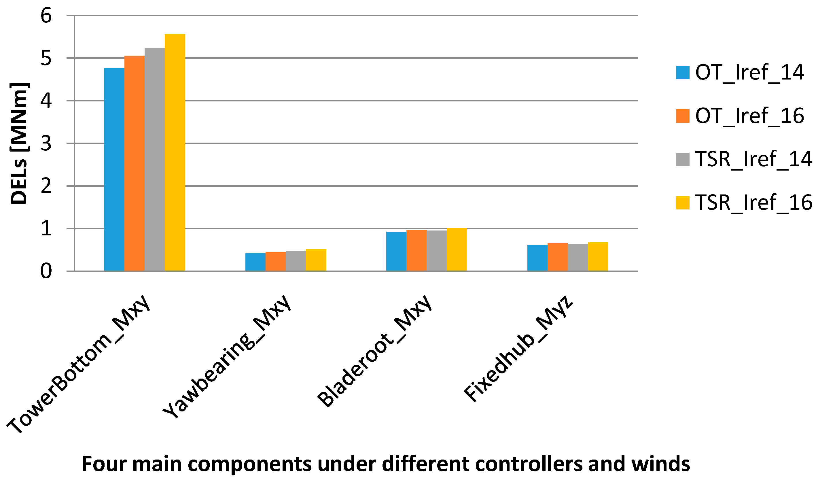Based on simulation results of these simulation cases, damage equivalent loads (DELs) were calculated based on the assumption that the WT lifetime is 20 years and the press cycle time is 1.0 × 10⁸. By using a Wohler exponent of 4 for steel, the DELs of four main components (including tower bottom, yaw bearing, fixed hub and blade root) were computed. According to the coordinate systems defined in Bladed, component loads can be calculated in three directions. In this paper, only the dominative DELs were provided to show for the sake of simplicity. For tower bottom, yaw bearing, and blade root, their DELs of Mxy were used, whereas, for the hub, the DEL of Myz was used. Their results are shown in Figure 11.

The results in Figure 11 show a similar trend that all component loads under two controllers were increased in a degree when the TI of wind speed increases. For the TSR controller, comparing to the results at TI of $I_{\mathrm{ref}}=0.14$, the DELs at TI of $I_{\mathrm{ref}}=0.16$ were increased about 6.2%, 9.2%, 4.5% and 6.5% for tower bottom Mxy, yaw bearing Mxy, blade root Mxy and fixed hub Myz, respectively, while for the OT controller, comparing to the results at TI of $I_{\mathrm{ref}}=0.14$, the DELs at TI of $I_{\mathrm{ref}}=0.16$ were increased about 6.1%, 9.2%, 6.2% and 5.9% for the same four components, respectively.

Meanwhile, it can be obviously seen that the component loads by the TSR controller were larger than the ones by the OT controller under same TIs. At TI of $I_{ref}=0.14$, by comparison to the results of the OT controller, DELs of the TSR controller were increased about 9.9%, 14.4%, 2.6% and 3.2% for tower bottom, yaw bearing, blade root and fixed hub, respectively. At TI of $I_{ref}=0.16$, by comparison to the results of the OT controller, DELs of the TSR controller were increased about 9.8%, 12.6%, 4.2% and 2.6% for the four components, respectively. The comparison results well fitted the fact that bigger variation of output power was caused by the TSR controller than its counterpart.

4.4. Result Discussions

It appears that over a wide range of the wind speed, the TSR controller outperformed the OT controller in terms of power production performance, but it had a power variation that induced large loads for WT’s components. Comparing results for dominative loads of four main components illustrated that the TSR controller gave a payback of load increments for its power production enhancement. Since fatigue loads and energy production performance are two indexes for evaluating a control algorithm, it can be seen that, for a large WT, the two MPPT controllers have different advantages.

Meanwhile, it is obvious that both controllers suffered from power reduction and power variation to a degree that is relevant to the mean value and TI of the wind speed: the power reduction is increased by the increased TI, whereas the power variation is increased by both the increased TI and the increased mean wind speed. The power reduction reason was revealed by the fact that the rotor speeds lagged behind the wind speeds and the TSR presented variations around the optimal value. Comparing to the OT method, the TSR method offers a fast response. However, both methods have the limitation that it is infeasible to further optimize wind energy capture performance for a large WT. To tackle this problem, a feasible way may be to apply wind speed prediction technology in a more advanced controller.

5. Conclusions

MPPT algorithm is indispensable for enhancing energy capture performance of WTs. It is important to understand capability of the MPPT control method before applying it. Meanwhile, it is also necessary to investigate the limitation of the existing MPPT control methods before researching new methods. In this paper, we compared two MPPT control methods: the OT method is the standard MPPT method, whereas the TSR method is the one under study. Most of the previous works have considered only the algorithm design, regardless of the fact that the control performance may be affected by the inertia of a large WT and the wind speed characteristics. We carried out simulations to investigate the performance of the two control methods in the presences of different wind speed characteristics.

To clearly show the investigation results, we provided different simulation results under five cases: Cases 1 and 2 were with a wind speed of mean value 6 m/s; Cases 3 and 4 were with a wind speed of mean value 8 m/s; and Case 5 was with a wind speed of mean value 10 m/s. Meanwhile, different turbulence intensities were used for each case. From the comparison results of the two controllers under different winds, we demonstrate that the TSR method outperforms the OT method in terms of power production, whereas the OT method is preferable in terms of component fatigue loads. The results can be used as a reference by wind turbine designers to determine the control algorithm depending on their preference, whether to maximize power output or optimize component loads. Besides, we find out that the two methods suffer from power reduction that is caused by a delayed response due to a large inertia. The delayed response issue is the main burden of further optimizing wind energy capture performance for a large WT, thus a feasible way may be to address advanced control methods that can take advantage of wind speed prediction information. Furthermore, it is worthy noting that when the ${\mathrm{C}}_{\mathrm{p}}$ parameters of a WT are unknown or uncertain, an adaptive method will be required to track the real MPP.

References

1. Global Wind Energy Council. Global Wind Statistics 2016. Available online: http://www.gwec.net/wp-content/uploads/vip/GWEC_PRstats2016_EN_WEB.pdf (accessed on 3 March 2017).
2. Lindenberg, S.; Smith, B.; O’Dell, K. 20% Wind Energy by 2030. Available online: http://asiapacificpartnership.org/pdf/PGTTF/wind-event/March_2/APP_20_Summary.pdf (accessed on 28 April 2017).
3. National Development and Reform Commission. Available online: http://finance.sina.com.cn/roll/2017-04-25/doc-ifyepnea4974841.shtml (accessed on 25 April 2017).
4. Chehouri, A.; Younes, R.; Ilinca, A.; Perron, J. Review of performance optimization techniques applied to wind turbines. Appl. Energy 2015, 142, 361–388. [Google Scholar] [CrossRef]
5. Tian, J.; Zhou, D.; Su, C.; Soltani, M.; Chen, Z.; Blaabjerg, F. Wind turbine power curve design for optimal power generation in wind farms considering wake effect. Energies 2017, 10, 395. [Google Scholar] [CrossRef]
6. Luo, X.; Niu, S.X. Maximum power point tracking sensorless control of an axial-flux permanent magnet vernier wind power generator. Energies 2016, 9, 581. [Google Scholar] [CrossRef]
7. Bonfiglio, A.; Delfino, F.; Invernizzi, M.; Procopio, R. Modeling and maximum power point tracking control of wind generating units equipped with permanent magnet synchronous generators in presence of losses. Energies 2017, 10, 102. [Google Scholar] [CrossRef]
8. Kumar, D.; Chatterjee, K. A review of conventional and advanced MPPT algorithms for wind energy systems. Renew. Sustain. Energy Rev. 2016, 55, 957–970. [Google Scholar] [CrossRef]
9. Zhong, Q.H.; Ruan, Y.; Zhao, M.H.; Tan, L. Application of variable-step hill climbing searching in maximum power point tracking for DFIG wind power generation system. Power Syst. Prot. Control 2013, 41, 67–73. [Google Scholar]
10. Pagnini, L.C.; Burlando, M.; Repetto, M.P. Experimental power curve of small-size wind turbines in turbulent urban environment. Appl. Energy 2015, 154, 112–121. [Google Scholar] [CrossRef]
11. Johnson, K.E.; Pao, L.Y.; Balas, M.J.; Fingersh, L.J. Control of variable-speed wind turbines: Standard and adaptive techniques for maximizing energy capture. IEEE Trans. Control Syst. 2006, 26, 70–81. [Google Scholar] [CrossRef]
12. Cheng, M.; Zhu, Y. The state of the art of wind energy conversion systems and technologies: A review. Energy Convers. Manag. 2014, 88, 332–347. [Google Scholar] [CrossRef]
13. Yang, J.; Song, D.R.; Dong, M.; Chen, S.F.; Zou, L.B.; Guerrero, J.M. Comparative studies on control systems for a two-blade variable-speed wind turbine with a speed exclusion zone. Energy 2016, 109, 294–309. [Google Scholar] [CrossRef]
14. Johnson, K.E.; Fingersh, L.J.; Balas, M.J.; Pao, L.Y. Methods for increasing region 2 power capture on a variable-speed wind turbine. J. Sol. Energy Eng. 2004, 126, 1092–1100. [Google Scholar] [CrossRef]
15. Johnson, K.E. Adaptive Torque Control of Variable Speed Wind Turbines; National Renewable Energy Laboratory: Golden, CO, USA, 2004.
16. Odgaard, P.F.; Damgaard, C.; Nielsen, R. On-line estimation of wind turbine power coefficients using unknown input observers. IFAC Proc. Vol. 2008, 41, 10646–10651. [Google Scholar] [CrossRef]
17. Yin, M.; Zhang, X.; Zou, Y.; Zhou, L. Improved MPPT control of wind turbines based on optimization of tracking range. Power Syst. Technol. 2014, 38, 2180–2185. [Google Scholar]
18. Zhang, X.L.; Huang, C.; Hao, S.P.; Chen, F.; Zhai, J.J. An improved adaptive-torque-gain MPPT control for direct-driven PMSG wind turbines considering wind farm turbulences. Energies 2016, 9, 977. [Google Scholar] [CrossRef]
19. Wang, N.; Johnson, K.E.; Wright, A.D. Comparison of strategies for enhancing energy capture and reducing loads using LIDAR and feedforward control. IEEE Trans. Control Syst. Technol. 2013, 21, 1129–1142. [Google Scholar] [CrossRef]
20. Schlipf, D.; Schlipf, D.J.; Kühn, M. Nonlinear model predictive control of wind turbines using LIDAR. Wind Energy 2013, 16, 1107–1129. [Google Scholar] [CrossRef]
21. Scholbrock, A.; Fleming, P.; Schlipf, D. Lidar-enhanced wind turbine control: Past, present, and future. In Proceedings of the American Control Conference, Boston, MA, USA, 6–8 July 2016; pp. 1399–1406. [Google Scholar]
22. Ahmed, G.; Abo, K.; Lee, D.C. MPPT control of wind generation systems based on estimated wind speed using SVR. IEEE Trans. Ind. Electron. 2008, 55, 1489–1490. [Google Scholar]
23. Boukhezzar, B.; Siguerdidjane, H. Nonlinear control of a variable-speed wind turbine using a two-mass model. IEEE Trans. Energy Convers. 2011, 26, 149–162. [Google Scholar] [CrossRef]
24. Soltani, M.N.; Knudsen, T.; Svenstrup, M.; Wisniewski, R.; Brath, P.; Ortega, R.; Johnson, K.E. Estimation of rotor effective wind speed: a comparison. IEEE Trans. Control Syst. 2013, 21, 1155–1167. [Google Scholar] [CrossRef]
25. Chen, Z.; Liu, A.; Li, A.; Choi, Y.; Li, J. Distributed duty cycle control for delay improvement in wireless sensor networks. Peer-to-Peer Netw. Appl. 2017, 10, 559–578. [Google Scholar] [CrossRef]
26. Song, D.R.; Yang, J.; Cai, Z.L.; Dong, M.; Su, M.; Wang, Y.H. Wind estimation with a non-standard extended Kalman filter and its application on maximum power extraction for variable speed wind turbines. Appl. Energy 2017, 190, 670–685. [Google Scholar] [CrossRef]
27. Tang, C.; Soong, W.L.; Freere, P.; Pathmanathan, M.; Ertugrul, N. Dynamic wind turbine output power reduction under varying wind speed conditions due to inertia. Wind Energy 2013, 16, 561–573. [Google Scholar] [CrossRef]
28. Yin, M.; Zhang, X.; Ye, X.; Zou, Y. Improved MPPT control based on the reduction of tracking range. Proc. CSEE 2012, 32, 24–31. [Google Scholar]
29. Garrad Hassan and Partners Ltd. GH Bladed User Manual; Garrad Hassan and Partners Ltd.: Bristol, UK, 2009. [Google Scholar]
30. Garrad Hassan and Partners Ltd. GH Bladed Theory Manual; Garrad Hassan and Partners Ltd.: Bristol, UK, 2009. [Google Scholar]
31. Blaabjerg, F.; Liserre, M.; Ma, K. Power electronics converters for wind turbine systems. IEEE Trans. Ind. Appl. 2011, 48, 281–290. [Google Scholar]
32. Chen, Z.; Guerrero, J.M.; Blaabjerg, F. A review of the state of the art of power electronics for wind turbines. IEEE Trans. Power Electron. 2009, 24, 1859–1875. [Google Scholar] [CrossRef]
33. Grewal, M.S.; Andrews, A.P. Kalman Filtering: Theory and Practice Using MATLAB, 2nd ed.; Wiley: New York, NY, USA, 2001. [Google Scholar]
34. Song, D.R.; Yang, J.; Dong, M.; Joo, Y.H. Kalman filter-based wind speed estimation for wind turbine control. Int. J. Control Autom. Syst. 2017, in press. [Google Scholar]
35. International Electro-technical Commission. IEC 61400-1 International Standard, Wind Turbines—Part 1: Design Requirements, 3rd ed.; International Electro-technical Commission: Geneva, Switzerland, 2005. [Google Scholar]
Figure 1. Energy conversion system diagram of the concerned WT.
Energies 10 00613 g001
Figure 2. Aerodynamic power coefficient curves of the concerned WT under different β and λ .
Energies 10 00613 g002
Figure 3. The two MPPT control structures: (a) the OT-based controller; and (b) the TSR-based controller.
Energies 10 00613 g003
Figure 4. Time dependence of the wind speed for: (a) Cases 1 and 2; (b) Cases 3 and 4; and (c) Case 5.
Energies 10 00613 g004
Figure 5. Simulation results under Case 1 with mean speed of 6 m/s and TI of 0.236.
Energies 10 00613 g005aEnergies 10 00613 g005b
Figure 6. Simulation results under Case 2 with mean wind speed of 6 m/s and TI of 0.269.
Energies 10 00613 g006
Figure 7. Simulation results under Case 3 with mean speed of 8 m/s and TI of 0.203.
Energies 10 00613 g007
Figure 8. Simulation results under Case 4 with mean speed of 6 m/s and TI of 0.232.
Energies 10 00613 g008
Figure 9. Simulation results under Case 5 with mean speed of 10 m/s and TI of 0.210.
Energies 10 00613 g009
Figure 10. Statistical results comparison for the two controllers under four cases: (a) the output power results; and (b) the TSR results.
Energies 10 00613 g010
Figure 11. DELs of four main components under the two controllers with different TI.
Energies 10 00613 g011