Bifurcation Phenomena Studies of a Voltage Controlled Buck-Inverter Cascade System

Abstract

This paper studies the complex bifurcation phenomena of a voltage-controlled Buck-inverter cascade system. A state-flow chart is drawn to illustrate the complex relations among the linear operating modes. Combined with the state transition function of each mode, the time response of the system can be obtained. For period-one steady state, the periodic mapping function and its fixed point are further derived, on the basis of which the Jacobi matrix is developed and its maximum eigenvalue is analyzed to understand the bifurcation diagram. By globally analyzing the state space using this cell mapping method, the coexistence of attractors is revealed in the Buck-inverter system. All theoretical results have been verified experimentally on a prototype system. The results obtained can be used for guiding the design and analysis of the Buck-inverter system. The analyzing method can be helpful for studying other power electronics systems with compound topologies.

1. Introduction

Buck-inverter cascade configuration is widely used in wireless power transfer (WPT) and inductive heating applications for high frequency magnetic field generation [1,2,3]. Usually, the inverter is used to drive a resonant network to generate high-frequency alternating current along the transmitter coil [2] or the heating coil [4], and the Buck converter is used to regulate the output power. However, due to the interactions between the Buck converter and the load resonant inverter, and the nonlinear switching effect of the switches, nonlinear characteristics are inevitable issues to consider when designing a Buck-inverter system [5].

In fact, nonlinear characteristics are common in power electronics systems. Various nonlinear phenomena in power electronics have been found in the past two decades. The initial research focused on DC/DC unit converters. Period-doubling bifurcation and chaos were found in Buck, Boost, Buck-Boost and Sepic converters, etc. [6,7,8,9,10,11,12]. Particularly, the coexistence of the attractor’s phenomenon was found in Buck converters. Starting from different initial values, the converters converged to different steady states [13,14]. Flip bifurcation and chaos were found in a three-state boost switching regulators, and the results show the system exhibited a typical route to chaos via period-doubling [15]. Later, nonlinear phenomena in AC/DC converters were studied. Reference [16] studied the fast-scale instability in a power-factor-correction (PFC) Boost converter, and bifurcation near the switching moment was observed. Nonlinear phenomena in DC/AC inverters were first studied in [17], and border collision bifurcation occurred when varying the control parameters. Furthermore, Hopf bifurcation was also observed in DC/AC inverters, and it has been verified that Hopf bifurcation is also a route to chaos [18]. Reference [19] studied chaos and the coexistence of attractors’ phenomena in a full-bridge converter. The results show that the period-one attractor co-exists with the period-three attractor at some critical parameter values. Moreover, there are also some studies of nonlinear behaviors in high-order converters [20,21,22]. Bifurcation and chaos were found in parallel Buck or Boost converters. Unlike parallel converters, the authors of [23,24] studied the nonlinear characteristics of a load resonant DC/DC combined converter, which is a cascade system with a DC/AC inverter series connected to an AC/DC converter, and a symmetry-breaking bifurcation was introduced in this research. All of the above studies showed that complex nonlinear phenomena can exist in various power electronics converters because of the switching transitions among different circuit topologies [24,25]. Studies on the nonlinear behaviors help us to better understand the operation principles of the power electronics systems and can furthermore lead to innovative techniques in dealing with the nonlinearities.

When analyzing the nonlinear phenomena of the converters, a discrete mapping modeling method is commonly used. The method can quickly determine the periodic state, so as to plot bifurcation diagrams [6,11,12]. For combined parallel and series converters, the nonlinear phenomena are much more complex than in single unit converters, which have been proven to be more difficult in being modeled and analyzed [26,27]. In this paper, to better analyze the operating principle of the Buck-inverter cascade system, a state-flow chart has been introduced to illustrate the complex relations among the linear operating modes. In order to globally analyze the coexistence of attractors, the cell mapping method is also introduced. Utilizing these methods, bifurcation diagrams with the reference voltage and the input voltage as bifurcation parameters are studied and verified by the maximum Jacobi matrix eigenvalues. In particular, the coexistence of attractors is observed theoretically and verified experimentally.

The paper is structured as follows: the operating principle, state-flow chart and Jacobi matrix analysis of the Buck-inverter system is derived in Section 2; bifurcation diagrams and theoretical verification by the maximum Jacobi matrix eigenvalues are shown in Section 3; the coexistence of attractors are revealed and investigated globally with the cell mapping analytical method in Section 4; the experiment verification of the bifurcation diagrams and coexistence of attractors are presented in Section 5; and finally, the conclusions are drawn in Section 6.

2. Modeling of Voltage-Controlled Buck-Inverter

2.1. Operating Principles of Voltage-Controlled Buck-Inverter

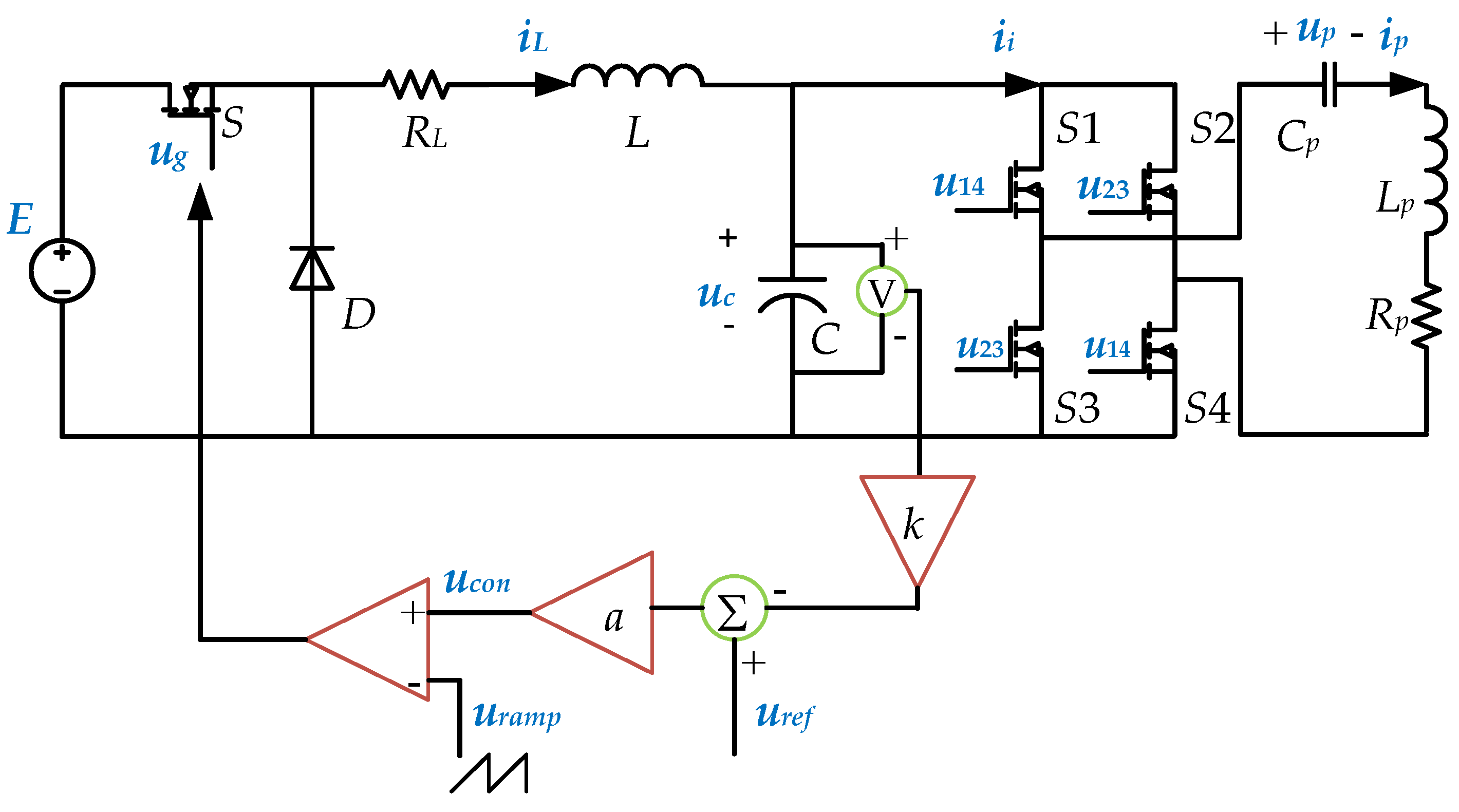
The diagram of the voltage-controlled Buck-inverter cascade system is shown in Figure 1. The main topology consists of two parts. One is a Buck converter and the other is a full-bridge load resonant inverter. A voltage closed loop is added to the output voltage of the Buck converter to adjust the output power of the system. E is the input DC source. S and D are the switch and the fly-wheeling diode of the Buck circuit, respectively. L and C constitute a low pass filter. R_L is the equivalent series resistance of L. S1, S2, S3 and S4 constitute a full-bridge inverter. L_p and C_p constitute a series resonant circuit to obtain a high frequency sinusoidal alternating current in the coil L_p. R_p is the equivalent load. To achieve a soft switching operating mode, switches S1–S4 should commutate at the instance when the current i_p crosses zero [28,29]. In the voltage feedback control loop, u_ref is the reference voltage and u_c is the output voltage of the Buck converter which is sensed by a voltage divider with a ratio of k and subtracted from the reference voltage u_ref. a is the gain of the error amplifier which can also be regarded as a proportional controller.

The control voltage u_con shown in Figure 1 can be written as:

$$u_{con}=a(u_{ref}-k{u}_c)$$

(1)

The saw-tooth carrier signal in one control period is given as:

$$u_{ramp}=U_L+(U_H-U_L)t,t\in \left[0,T_b\right]$$

(2)

where t is the time variable; T_b (T_b = 1/f_b, f_b is the frequency of the Buck converter) is the period of the saw-tooth signal; U_L and U_H are its lower and upper threshold values respectively.

The negative voltage feedback control strategy of the Buck circuit is:

$$u_g=\{\begin{array}{c}1u_{con}\ge u_{ramp}\\ 0u_{con}<u_{ramp}\end{array}$$

(3)

To achieve soft switching, a fixed frequency which is consistent with the natural frequency of the resonant network is used to control the inverter. The control sequence in one period can be written as:

$$\{\begin{array}{c}{u}_{14}=1,u_{23}=0,t\in \left[0,\frac{T_i}{2}\right]\\ u_{23}=1,u_{14}=0,t\in \left(\frac{T_i}{2},T_i\right]\end{array}$$

(4)

where t is the time variable, and T_i (T_i = 1/f_i, f_i is the frequency of the resonant inverter) is the control period of the resonant inverter.

2.2. State-Flow Chart of Buck-Inverter System

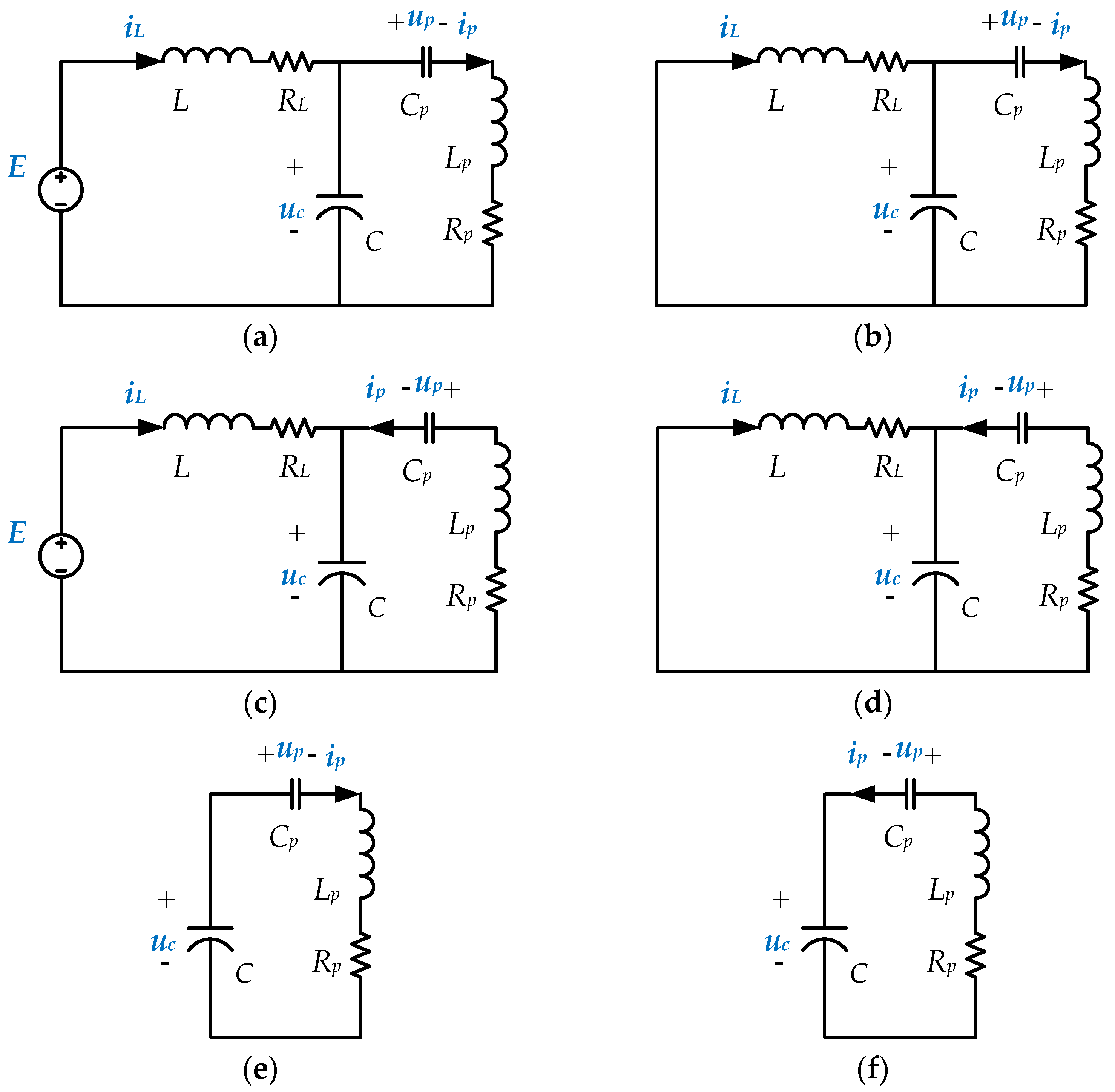
Usually, when analyzing power electronics systems, we divide the system into a series of operation modes according to the on/off state of the controlled and non-controlled switches and study the modes one by one [30,31]. Accordingly, the Buck-inverter system shown in Figure 1 can be piecewise linearized into six possible working modes because the Buck converter works in continuous current mode (CCM) and discontinuous current mode (DCM):

(1)

Mode 1: S, S1, S4 on and D, S2, S3 off;

(2)

Mode 2: D, S1, S4 on and S, S2, S3 off;

(3)

Mode 3: S, S2, S3 on and D, S1, S4 off;

(4)

Mode 4: D, S2, S3 on and S, S1, S4 off;

(5)

Mode 5: S1, S4 on and S, D, S2, S3 off;

(6)

Mode 6: S2, S3 on and S, D, S1, S4 off.

The equivalent circuits of these six working modes are shown in Figure 2a–f respectively.

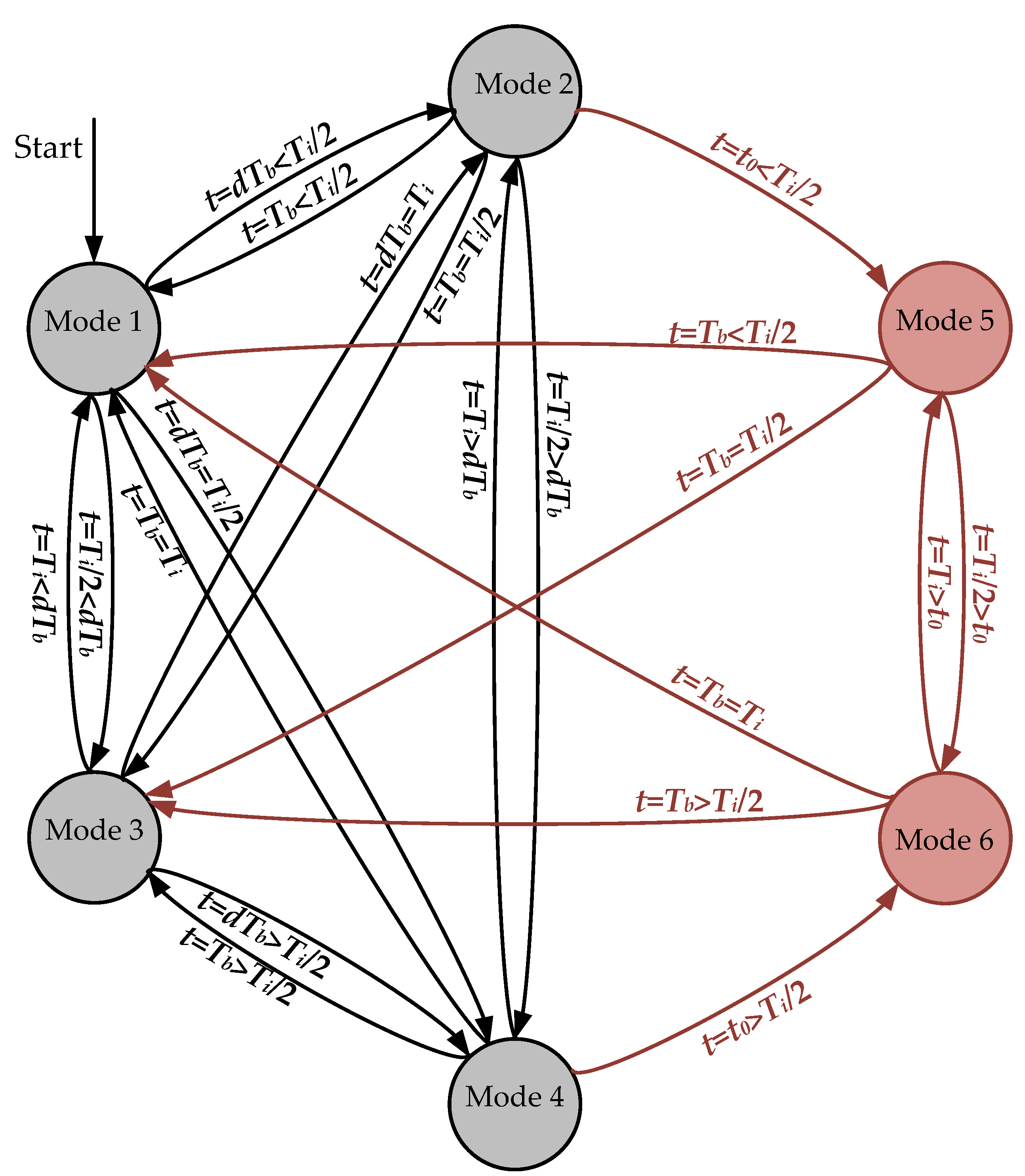
To reveal the complex relations among the working modes, the state-flow chart of the six working modes is drawn and shown in Figure 3, where t₀ is the time when i_L falls to zero when the Buck converter works in DCM. d is the duty cycle of Buck converter. The system starts from Mode 1. The direction of the arrows indicates the flow of the working modes, while the texts on the arrows indicate the mode switching conditions. Black lines indicate the flow cases when only considering the CCM of the Buck converter, while red lines indicate the further flow cases when considering the DCM of the Buck converter.

Choose X = [i_L u_c i_p u_p]^T and U = [E] as the state vector and the input vector of the Buck-inverter respectively. Then the state space model of these six working modes can be derived according to Kirchhoff’s law:

$$\{\begin{array}{c}\dot{X}=A_{1}X+B_{1}U,\mathrm{Mode}1\\ \dot{X}=A_{2}X+B_{2}U,\mathrm{Mode}2\\ \dot{X}=A_{3}X+B_{3}U,\mathrm{Mode}3\\ \dot{X}=A_{4}X+B_{4}U,\mathrm{Mode}4\\ \dot{X}=A_{5}X+B_{5}U,\mathrm{Mode}5\\ \dot{X}=A_{6}X+B_{6}U,\mathrm{Mode}6\end{array}$$

(5)

where A₁ = A₂ = $\left[\begin{array}{cccc}\frac{-R_L}{L}& \frac{-1}{L}& 0& 0\\ \frac{1}{C}& 0& \frac{-1}{C}& 0\\ 0& \frac{1}{L_P}& \frac{-R_p}{L_P}& \frac{-1}{L_P}\\ 0& 0& \frac{1}{C_P}& 0\end{array}\right]$, A₃ = A₄ = $\left[\begin{array}{cccc}\frac{-R_L}{L}& \frac{-1}{L}& 0& 0\\ \frac{1}{C}& 0& \frac{1}{C}& 0\\ 0& \frac{-1}{L_P}& \frac{-R_p}{L_P}& \frac{-1}{L_P}\\ 0& 0& \frac{1}{C_P}& 0\end{array}\right]$, A₅ = $\left[\begin{array}{cccc}0& 0& 0& 0\\ 0& 0& \frac{-1}{C}& 0\\ 0& \frac{1}{L_P}& \frac{-R_p}{L_P}& \frac{-1}{L_P}\\ 0& 0& \frac{1}{C_P}& 0\end{array}\right]$, A₆ = $\left[\begin{array}{cccc}0& 0& 0& 0\\ 0& 0& \frac{1}{C}& 0\\ 0& \frac{-1}{L_P}& \frac{-R_p}{L_P}& \frac{-1}{L_P}\\ 0& 0& \frac{1}{C_P}& 0\end{array}\right]$, B₁ = B₃ = $\left[\begin{array}{c}\frac{1}{L}\\ 0\\ 0\\ 0\end{array}\right]$, B₂ = B₄ = B₅ = B₆ = $\left[\begin{array}{c}0\\ 0\\ 0\\ 0\end{array}\right]$.

The analytical solution of each linearized mode can be described as follows according to [32]

$$X\left(t\right)=\{\begin{array}{ll}{\Phi }_1\left(t\right)X_{10}+\left({\Phi }_1\left(t\right)-I\right){A_1}^{-1}{B}_{1}E& \mathrm{Mode}1\\ {\Phi }_2\left(t\right)X_{20}& \mathrm{Mode}2\\ {\Phi }_3\left(t\right)X_{30}+\left({\Phi }_3\left(t\right)-I\right){A_3}^{-1}{B}_{3}E& \mathrm{Mode}3\\ {\Phi }_4\left(t\right)X_{40}& \mathrm{Mode}4\\ {\Phi }_5\left(t\right)X_{50}& \mathrm{Mode}5\\ {\Phi }_6\left(t\right)X_{60}& \mathrm{Mode}6\end{array}$$

(6)

where i (i = 1, 2, 3, 4, 5, 6) is the mode number and Φ_i (t) = e^Ait, X_i0 is the initial states of each working mode.

According to the mode transition chart shown in Figure 3 and the state transition function of each working mode shown in Equation (6), the dynamical time responses of the Buck-inverter system can be derived for any given initial states with the strategies of the Buck converter and the resonant inverter as shown in Equations (3) and (4).

As discussed in [32], if the steady state mode series are known, the steady state responses are able to be predicted analytically. However, for the Buck-inverter cascade system, if T_b is different from T_i, the steady state mode series will be unknown especially when T_b and T_i are relatively prime. In this case, the steady state periodic mapping function cannot be derived and neither can the Jacobi matrix. The nonlinearity of the system can only be studied through numerical simulations. In order to better understand the bifurcation characteristics of the system, we assume T_b = T_i and the phase difference is zero in the following sections.

2.3. Stability Analysis of Period-One Steady State

The maximum Jacobi matrix eigenvalue is an effective way to verify the stability of the system at period-one steady state [33,34]. If the absolute value of the maximum Jacobi matrix eigenvalue is larger than 1, the period-one operating point is unstable (there is bifurcation or chaos).

To simplify, assume that the Buck converter works in CCM, since the analysis process is the same when Buck works in DCM. When the Buck converter goes into period-one steady state, the state flow is different from when the duty cycle d of the Buck converter is larger or smaller than 0.5. When d is larger than 0.5, the state flow in the steady period is: Mode 1, Mode 3, Mode 4. And the time spans of the three modes are ξ₁ = T_b/2, ξ₃ = dT_b − T_b/2 and ξ₄ = T_b − dT_b respectively. When time variable t is smaller than T_b/2, the Buck-inverter works in Mode 1, and then it goes into Mode 3 when t = T_b/2. Finally, the system goes into Mode 4 when t = dT_b. Otherwise, when d is smaller than 0.5, the state-flow in the steady period is: Mode 1, Mode 2, Mode 4. And the time spans of the three modes are ξ₁ = dT_b, ξ₂ = T_b/2 − dT_b and ξ₄ = T_b/2 respectively. When the time variable t is smaller than dT_b, the Buck-inverter works in Mode 1, and then goes into Mode 2 when t = dT_b. Finally, the system goes into Mode 4 when t = T_b/2.

The analytical solution of each linearized mode in one period can be described as follows when d is larger or smaller than 0.5.

$$\begin{array}{l}d\ge 0.5:X\left(t\right)=\{\begin{array}{ll}{\Phi }_1\left(t\right)X_0+\left({\Phi }_1\left(t\right)-I\right){A_1}^{-1}{B}_{1}E& t\in \left[0,\frac{T_b}{2}\right]\\ {\Phi }_3\left(t-\frac{T_b}{2}\right)X\left(\frac{T_b}{2}\right)+\left({\Phi }_3\left(t-\frac{T_b}{2}\right)-I\right){A_3}^{-1}{B}_{3}E& t\in \left(\frac{T_b}{2},d{T}_b\right]\\ {\Phi }_4\left(t-d{T}_b\right)X\left(d{T}_b\right)& t\in \left(d{T}_b,T_b\right]\end{array}\\ d<0.5:X\left(t\right)=\{\begin{array}{ll}{\Phi }_1\left(t\right)X_0+\left({\Phi }_1\left(t\right)-I\right){A_1}^{-1}{B}_{1}E& t\in \left[0,d{T}_b\right]\\ {\Phi }_2\left(t-d{T}_b\right)X\left(d{T}_b\right)& t\in \left(d{T}_b,\frac{T_b}{2}\right]\\ {\Phi }_4\left(t-\frac{T_b}{2}\right)X\left(\frac{T_b}{2}\right)& t\in \left(\frac{T_b}{2},T_b\right]\end{array}\end{array}$$

(7)

where i (i = 1, 2, 3, 4) is the mode number, X₀ = X(_t)|_t=0 and Φ_i (t) = e^Ait.

Equation (7) results in six discrete mapping functions:

$$f_{i,\xi i}\left(X\right)={\Phi }_i\left({\xi }_i\right)X+A_i^{-1}\left({\Phi }_i\left({\xi }_i\right)-I\right)B_{i}Ui=1,2,3,4.$$

(8)

Let X₀ be the initial state and n = 0, 1, 2, . . . be the index of the discrete map. X_n and X_n+1 are the initial state and final state of each operating period, respectively. The duty cycle between the n to n + 1 interval is d_n, then ξ₁ = T_b/2, ξ₃ = d_nT_b − T_b/2 and ξ₄ = T_b − d_nT_b when d is larger than 0.5 while ξ₁ = d_nT_b, ξ₂ = T_b/2 − d_nT_b and ξ₄ = T_b − T_b/2 when d is smaller than 0.5. Based on (8), the stroboscopic mapping model F can be obtained as:

$$\begin{array}{ll}d\ge 0.5:X_{n+1}& =F\left(X_n,{\xi }_1,{\xi }_3,{\xi }_4\right)=f_{4,\xi 4}\circ f_{3,\xi 3}\circ f_{1,\xi 1}\left(X_n\right)\\ & ={\Phi }_4\left({\xi }_4\right)\left({\Phi }_3\left({\xi }_3\right)\left({\Phi }_1\left({\xi }_1\right)X_n+\left({\Phi }_1\left({\xi }_1\right)-I\right)A_1^{-1}{B}_{1}U\right)+\left({\Phi }_3\left({\xi }_3\right)-I\right)A_3^{-1}{B}_{3}U\right)\\ d<0.5:X_{n+1}& =F\left(X_n,{\xi }_1,{\xi }_2,{\xi }_4\right)=f_{4,\xi 4}\circ f_{2,\xi 2}\circ f_{1,\xi 1}\left(X_n\right)\\ & ={\Phi }_4\left({\xi }_4\right)\left({\Phi }_2\left({\xi }_2\right)\left({\Phi }_1\left({\xi }_1\right)X_n+\left({\Phi }_1\left({\xi }_1\right)-I\right)A_1^{-1}{B}_{1}U\right)\right)\end{array}$$

(9)

where f ◦ g(t) = f(g(t)).

Since the closed loop control of voltage is used in the Buck converter, the switching function S(X_n,d_n) can be derived as:

$$\begin{array}{l}d\ge 0.5:\\ S\left(X_n,d_n\right)\stackrel{def}{=}a\left(u_{ref}-k{\rm P}X\left(d_n{T}_b\right)\right)-\left(\alpha +\beta d_n\right)\\ =a\left(u_{ref}-k{\rm P}\left(\left({\Phi }_3\left({\xi }_3\right)\left({\Phi }_1\left({\xi }_1\right)X_n+\left({\Phi }_1\left({\xi }_1\right)-I\right)A_1^{-1}{B}_{1}U\right)+\left({\Phi }_3\left({\xi }_3\right)-I\right)A_3^{-1}{B}_{3}U\right)\right)\right)-\left(\alpha +\beta d_n\right)\\ d<0.5:\\ S\left(X_n,d_n\right)\stackrel{def}{=}a\left(u_{ref}-k{\rm P}X\left(d_n{T}_b\right)\right)-\left(\alpha +\beta d_n\right)\\ =a\left(u_{ref}-k{\rm P}\left({\Phi }_1\left({\xi }_1\right)X_n+\left({\Phi }_1\left({\xi }_1\right)-I\right)A_1^{-1}{B}_{1}U\right)\right)-\left(\alpha +\beta d_n\right)\end{array}$$

(10)

where X_n is the initial state of period n (n ∈ N); k is voltage divider ratio; a is the gain of the error amplifier; vector P = [0100] is a selection matrix of the Buck converter output voltage, α = U_L, β = U_H − U_L. The on and off state of the switch S should change at the moment S(X_n,d_n) = 0.

As can be seen from Equation (10), when the initial state of period n is determined, the duty cycle of the mapping period can be derived, and then according to Equation (9), the discrete mapping of the system can be obtained.

As mentioned before, the maximum Jacobi matrix eigenvalue is used to study the stability of the system at period-one steady state. The states repeat periodically when the system operates in period-one [32], i.e., X_n+1 = X_n. So the periodic fixed point can be derived as:

$$\begin{array}{l}d\ge 0.5:\\ x^{*}={\left(I-{\Phi }_4\left(\frac{T_b}{2}\right){\Phi }_1\left(\frac{T_b}{2}\right)\right)}^{-1}{\Phi }_4\left(T_b-d_n{T}_b\right)\left({\Phi }_3\left(\frac{2d_n{T}_b-T_b}{2}\right)\left({\Phi }_1\left(\frac{T_b}{2}\right)-I\right){A_1}^{-1}{B}_{1}E+\left({\Phi }_3\left(\frac{2d_n{T}_b-T_b}{2}\right)-I\right){A_3}^{-1}{B}_{3}E\right)\\ d<0.5:\\ x^{*}={\left(I-{\Phi }_4\left(\frac{T_b}{2}\right){\Phi }_1\left(\frac{T_b}{2}\right)\right)}^{-1}{\Phi }_4\left(\frac{T_b}{2}\right)\left({\Phi }_2\left(\frac{T_b}{2}-d_n{T}_b\right)\left({\Phi }_1\left(d_n{T}_b\right)-I\right)\right){A_1}^{-1}{B}_{1}E\end{array}$$

(11)

According to Equations (9) and (10), the Jacobi matrix can be derived, as Equation (12) shows, when d is larger than 0.5 [35]:

$$J\left(X_n\right)=\frac{\partial F}{\partial X_n}-\frac{\partial F}{\partial d_n}{\left(\frac{\partial S}{\partial d_n}\right)}^{-1}\left(\frac{\partial S}{\partial X_n}\right)$$

(12)

where $\frac{\partial F}{\partial X_n}={\Phi }_4\left(\frac{T_b}{2}\right){\Phi }_1\left(\frac{T_b}{2}\right)$, $\frac{\partial F}{\partial d_n}=T_b{\Phi }_4\left(T_b-d_n{T}_b\right)B_{3}E$, $\frac{\partial S}{\partial X_n}=-ak\mathrm{P}{\Phi }_3\left(\frac{2d_n{T}_b-T_b}{2}\right){\Phi }_1\left(\frac{T_b}{2}\right)$,

$$\frac{\partial S}{\partial d_n}=-ak\mathrm{P}\left(A_3{T}_b{\Phi }_3\left(\frac{2d_n{T}_b-T_b}{2}\right)\left({\Phi }_1\left(\frac{T_b}{2}\right)X_n+\left({\Phi }_1\left(\frac{T_b}{2}\right)-I\right){A_1}^{-1}{B}_{1}E\right)+T_b{\Phi }_3\left(\frac{2d_n{T}_b-T_b}{2}\right)B_{3}E\right)-\beta$$

When d is smaller than 0.5, the Jacobi matrix can be derived as:

$$J\left(X_n\right)=\frac{\partial F}{\partial X_n}-\frac{\partial F}{\partial d_n}{\left(\frac{\partial S}{\partial d_n}\right)}^{-1}\left(\frac{\partial S}{\partial X_n}\right)$$

(13)

where $\frac{\partial F}{\partial X_n}={\Phi }_4\left(\frac{T_b}{2}\right){\Phi }_1\left(\frac{T_b}{2}\right)$, $\frac{\partial F}{\partial d_n}=T_b{\Phi }_1\left(\frac{T_b}{2}-d_n{T}_b\right)B_{1}E$, $\frac{\partial S}{\partial X_n}=-ak\mathrm{P}{\Phi }_1\left(d_n{T}_b\right)$,

$$\frac{\partial S}{\partial d_n}=-ak\mathrm{P}\left(A_1{T}_b{\Phi }_1\left(d_n{T}_b\right)X_n+T_b{\Phi }_1\left(d_n{T}_b\right)B_{1}E\right)-\beta$$

Substituting Equations (11)–(13), the maximum Jacobi matrix eigenvalues can be obtained at the periodic fixed point, from which the stability of the system can be derived.

3. Bifurcation Studies of Buck-Inverter and Maximum Jacobi Matrix Eigenvalue Verification

In this section, bifurcation diagrams of the Buck-inverter will be presented and verified by the Jacobi matrix eigenvalue. The parameters of the system are shown in

Table 1. Parameters of the system.

Parameter	Value	Parameter	Value
L	99.39 µH	a	1
C	48.6 µF	Lp	327.84 µH
RL	0.7 Ω	Cp	193.16 nF
fb	20 kHz	Rp	2.19 Ω
fi	20 kHz	UL	1 V
k	1	UH	4 V

.

Bifurcation diagrams are a typical tool for analyzing nonlinear dynamic behaviors. Usually, it is obtained by stroboscopic sampling, and plotted between the input sensitive parameter in the X-axis and the behavior of a state space variable in the Y-axis [36]. Herein, the inductor current i_L is taken as the state variable, while the reference voltage u_ref and the input voltage E are taken as the sensitive parameters.

In order to obtain the bifurcation diagram, a stroboscopic sampling algorithm was added to the time responses of the system to pick out the data at the beginning of each operating period T_b (T_b = T_i) of i_L. For each set of sensitive parameter, 100 data points were sampled when the system was running in steady state. The initial states of each set of sensitive parameters are the steady state of the previous (For example, when we derived the time response when u_ref = 13 V, the previous u_ref is 12.9 V. 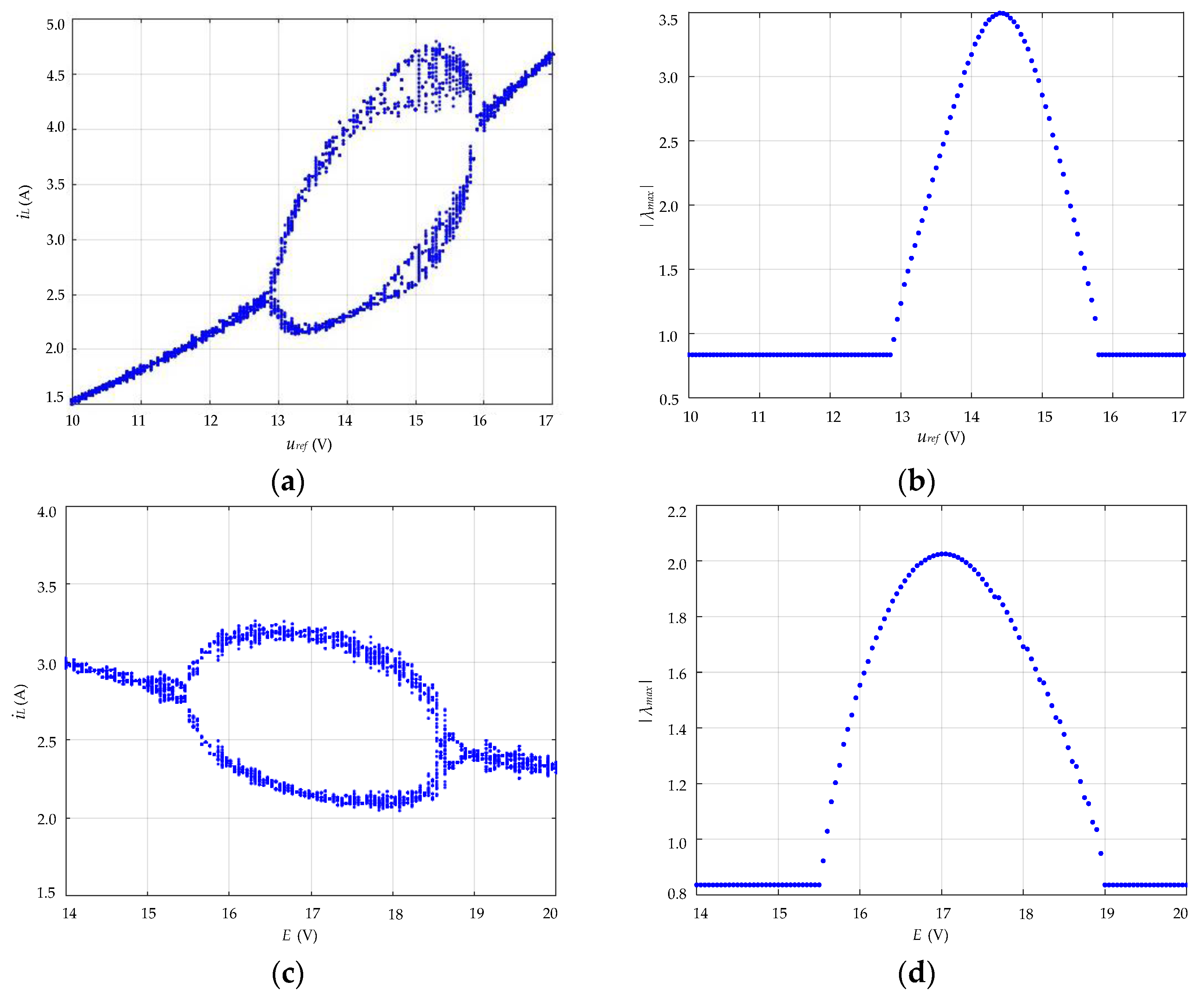We just took the steady state (not zero vector) when u_ref = 12.9 V as the initial state). The obtained bifurcation diagram is shown in Figure 4, where Figure 4a,c take u_ref and E as the sensitive parameters respectively (In Figure 4a, E is set to be 20 V while u_ref is set to be 12.5 V in Figure 4c).

As can be seen from Figure 4a, as the reference voltage u_ref increases, complex bifurcation occurs. The system exhibits period-one behavior for low values of u_ref, which remains stable up to u_ref ≈ 12.8 V. Then it bifurcates into period-two operating mode. This dynamic lasts up to u_ref ≈ 14.5 V and transits to period-four orbits from u_ref ≈ 14.5 V to 15.8 V except for a chaotic window at about 15.1 V to 15.8 V. At u_ref ≈ 15.8 V, the system goes back to period-one and lasts up to 17 V. As for the bifurcation diagram shown in Figure 4c, bifurcation occurs at about E ≈ 15.5 V, and goes back to period-one at E ≈ 18.8 V.

Figure 4b,d shows the maximum Jacobi matrix eigenvalue of the system with respect to the sensitive parameters. As can be seen from Figure 4b,d, the maximum Jacobi matrix eigenvalue only considers the stability of the periodic fixed point, and cannot determine whether the system is bifurcation or chaos when the absolute value is larger than 1. Comparing Figure 4a–d, the bifurcation diagrams correspond well to the maximum Jacobi matrix eigenvalues, and the unstable states (bifurcation of chaos) occur when the absolute value of the maximum Jacobi matrix eigenvalue is larger than 1. So the bifurcation diagrams are verified by the maximum Jacobi matrix eigenvalue, and this accuracy is further verified by the results of the experiment.

4. Cell Mapping Method and the Coexistence of Attractors of the Buck-Inverter

Initial sensitivity and parameter sensitivity are two typical properties of nonlinear systems [36]. Above, the bifurcation diagrams in Figure 4a,c show the parameter sensitivity of the Buck-inverter that the system converges to different steady states (e.g., period-one, period-two or chaos) when u_ref and E varies. In this section, we will study the initial states sensitivity of the Buck-inverter, considering that the system starts from different initial states (as mentioned before, the bifurcation diagrams shown in Figure 4a,c are derived by setting the steady state of the previous parameters as the initial states). References [13,14,19] show that the Buck converter and inverter have coexistence of attractors, and that the attractors are different corresponding to different initial values. As for the Buck-inverter, there are four state variables. In order to find the attractors quickly, we here introduce an analytical method: the cell mapping method.

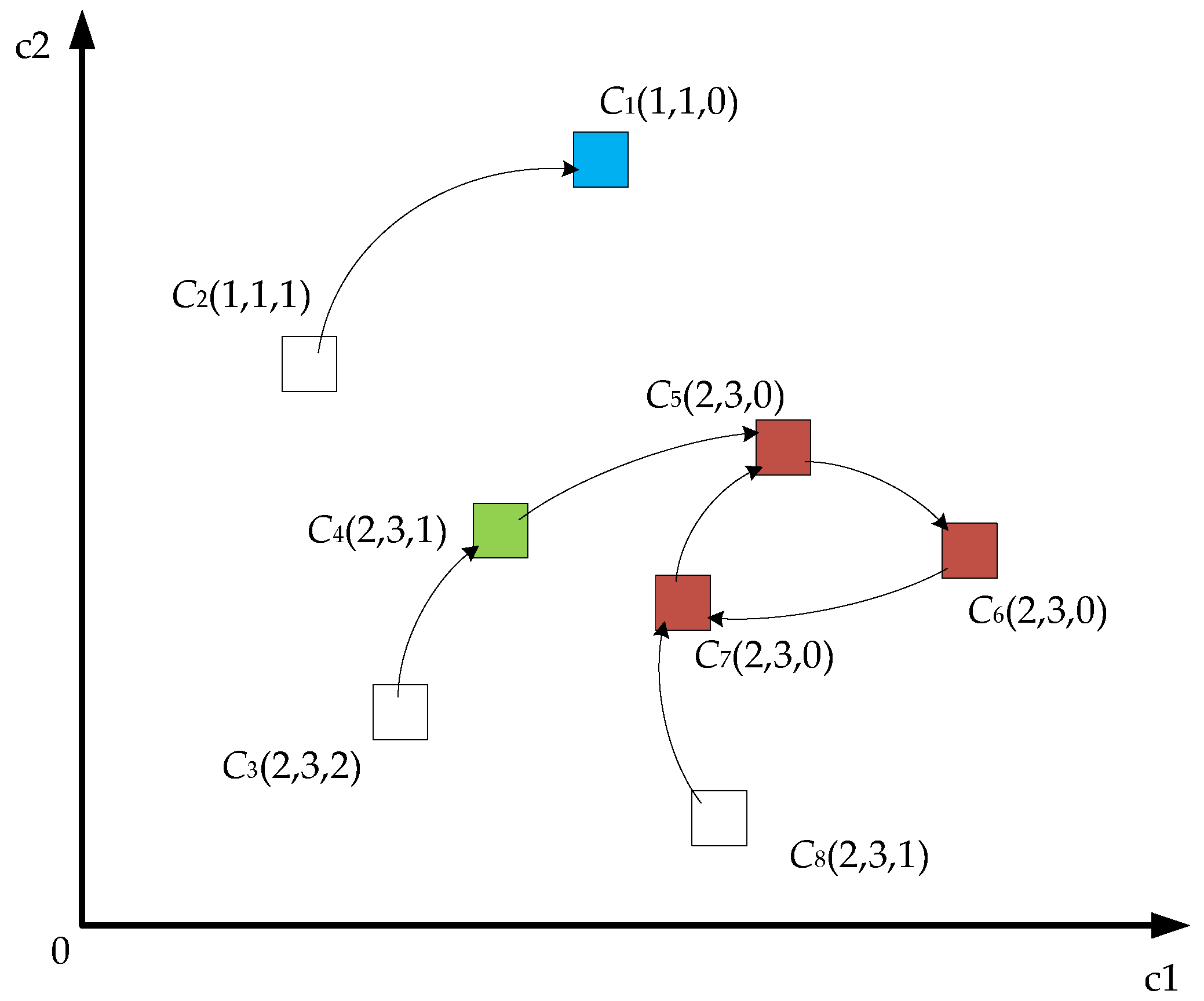
The cell mapping method can be used to find the domain of a nonlinear system [37]. Since there is no need to repeat the calculations when the cell enters into a known cell, the method can find the domain quickly. To help understand the cell mapping method, a two-dimension system is used to illustrate. Firstly, the cell can be defined as C_c(i,p,s), where c indicates the cell number, i, p and s indicate the index of the attractors, the period number and steps to enter the period, respectively.

The cell mapping process is shown in Figure 5, where C₅, C₆ and C₇ of red blocks indicate a period-three cycle with the step as zero, while C₄ (the green block) indicates a way to period-three with the step as one. C₁ (the blue block) indicates a period-one cycle with the step as zero. Considering the cell C₂, C₃ and C₈ of white blocks, C₃ and C₈ can also be the way to a period-three cycle, with the difference being that C₃ need two steps to get to the period-three cycle, while C₈ needs one step. C₂ is the way to period-one, and the step is one.

As mentioned above, cell mapping is a quick and effective way to search the domain of the attractors, assuming the colorful blocks C₁, C₄, C₅, C₆, C₇ are known cells, so C₂, C₃ and C₈ need only one step to derive the overall trajectory. For example, C₃ mapping to C₄ needs one step, so we can derive that C₃ belong to period-three domain, since C₄, C₅, C₆ and C₇ all belong to the period-three domain, so we do not need to repeat the mapping, e.g., mapping from C₄ to C₅.

As the parameters of the Buck-inverter has been determined in Table 1, the possible attractors can also be quickly derived. Set u_ref = 11, 12.5 and 16.6 V and E = 20 V, the possible initial value ranges are derived from the simulation study, and this is also verified by the results of the experiment: i_L = [0, 8] A; u_c = [0, 20] V; i_p = [−10, 10] A; u_p = [−300, 300] V. Then we divide the coordinate axis (i_L, u_c, i_p, u_p) into a countable number of intervals with uniform size (the uniform size may be different with respect to different axes), and assume the intervals belong to same domain of attractors. Here, we divide i_L, u_c, i_p and u_p into 8, 20, 21 and 61 intervals, so that the entire cell number is 204,960, and then we can derive the possible attractors of the global domain, and derive the cell numbers of different attractors. The results are shown in

Table 2. Cell numbers and attractors of different u_ref.

uref	Attractors	Cell Numbers
11 V	Period-one	204,960
12.5 V	Period-one	116,473
	Period-three	70,974
	Others	17,513
16.6 V	Period-one	102,467
	Period-three	47,625
	Period-four	35,219
	Others	19,649

, where the “Others” indicates that the period is beyond the maximum searching period (in this paper, the maximum searching period is set to be 10), or the steady state is chaos. It should be noted that the states of chaos are stochastic, so in the experimental verification section, we only cared about the period attractors.

As can be seen from Table 2, only period-one attractors exist in the system when u_ref = 11 V, while the coexistence of period-one and period-three attractors happens in the system when u_ref = 12.5 V, and coexistence of period-one, period-three and period-four attractors appears in the system when u_ref = 16.6 V. These attractors are verified by the results of the experiment.

5. Experimental Verification

To verify the bifurcation diagrams and coexistence of attractors as shown above, an experiment prototype was built with the measured main parameters shown in Table 1.

With the input disturbance (which is a change of the initial values by disturbance), the coexistence of attractors can be found. Normally, if the system has only one steady state, the different initial values will definitely lead the system to the same steady state. However, if the system has a coexistence of attractors, then the steady states are not the same.

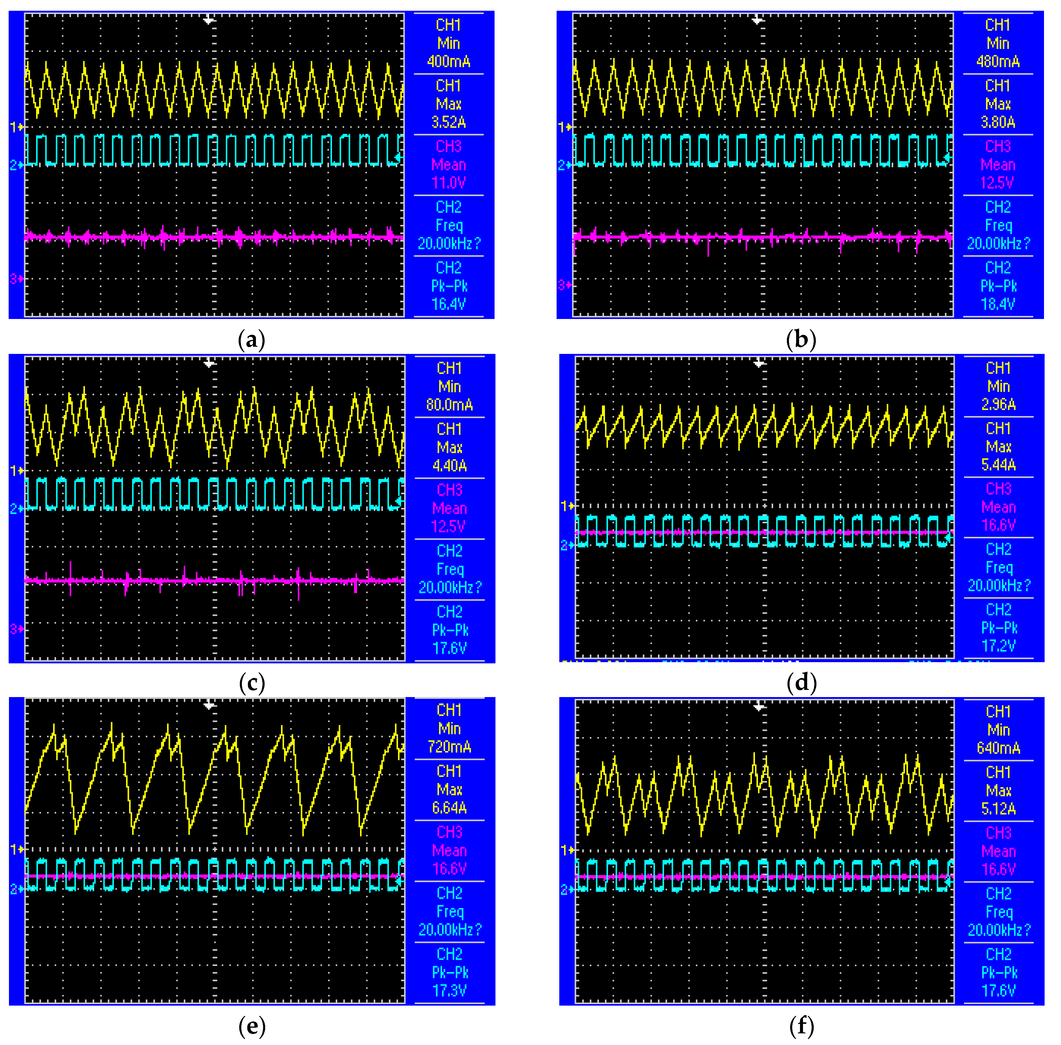
Three points mentioned in Section 4 of u_ref, i.e., 11 V, 12.5 V and 16.6 V, have been tested. The experiment results are shown in Figure 6a–f respectively. Where channel 1 is the inductor current i_L. channel 2 is the control signal of switch S1. Channel 3 is the reference voltage u_ref.

It can be seen from Figure 6 that the coexistence of attractors really exists in the Buck-inverter. Figure 6b,c show that when u_ref = 12.5 V, the system may result in period-one orbit or period-three orbit with different initial values. Figure 6d–f show that when u_ref = 16.6 V, the system may result in period-one orbit or period-three orbit or period-four orbit with different initial values. As for u_ref = 11 V, only period-one attractors in the system are shown in Figure 6a. Compared with the theoretical results shown in Figure 4 and Table 2, it can be seen that the bifurcation characteristics and coexistence of attractors match very well. So the bifurcation diagrams and coexistence of attractors are verified.

6. Conclusions

This paper studies the bifurcation phenomena of a voltage-controlled Buck-inverter cascade system. A state-flow chart has been introduced to illustrate the complex relations among the linear operating modes, on the basis of which the time responses of the system have been derived. The bifurcation diagrams have been obtained with respect to the reference voltage and the input voltage, and verified by the maximum Jacobi matrix eigenvalues. Specifically, the coexistence of attractors has been revealed and investigated globally utilizing the cell mapping method of analysis. Both the bifurcation diagrams and the coexistence of attractors have been verified by the experiment results.

It can be concluded that in a cascade power electronics system, complex nonlinear behaviors may exist. When we design such systems, the method presented in this paper can be applied to learn their bifurcation characteristics in the full range of variations of the key parameters such as load, input voltage and reference voltage, etc. Then boundaries of operation can be defined by checking the system in the bifurcation zone as to whether the performance requirements can be satisfied or not. Parameter optimization or specific control strategies dealing with the nonlinear phenomena should be further investigated and implemented if the system performance cannot meet the requirements.