A Generic Matrix Method to Model the Magnetics of Multi-Coil Air-Cored Inductive Power Transfer Systems ^†

Abstract

This paper deals with a generic methodology to evaluate the magnetic parameters of contactless power transfer systems. Neumann’s integral has been used to create a matrix method that can model the magnetics of single coils (circle, square, rectangle). The principle of superposition has been utilized to extend the theory to multi-coil geometries, such as double circular, double rectangle and double rectangle quadrature. Numerical and experimental validation has been performed to validate the analytical models developed. A rigorous application of the analysis has been carried out to study misalignment and hence the efficacy of various geometries to misalignment tolerance. The comparison of single-coil and multi-coil inductive power transfer systems (MCIPT) considering coupling variation with misalignment, power transferred and maximum efficiency is carried out.

1. Introduction

Inductive power transfer (IPT) relies on electromagnetic fields to transfer energy between circuits that are not physically connected. Loosely-coupled coils that are used in IPT systems suffer from high leakage fields that demand reactive power, constricting large power transfer at high efficiency. To nullify this effect, capacitive compensation is carried out such that reactive power exchange takes places between the capacitors and inductors with the source directly connected to the load, improving the power factor, power transfer and efficiency.

Inductive power transfer systems due to their non-contact nature allow efficient power flow to happen with reduced maintenance, being safe, clean and reliable. Thus, applications spanning from low power medical devices (mW) to mining (MW) have been found in the literature [1]. Other applications include consumer electronics, EVs, underwater power delivery, etc. [2,3]. A number of resonant topologies has been proposed, and several coil shapes and designs have been researched in this field [1]. However, an analytical framework that studies the impact of coil shape and misalignment in IPT systems in a rigorous manner is missing.

The magnetic design and its optimization are important steps in the design of IPT systems. Typically, coil optimization and magnetic parameter estimation $(L_1,L_2,M,k)$ are performed relying on electromagnetic (EM) field solvers and/or combing with evolutionary algorithms [4,5]. In other work, numerical techniques (solving look-up tables (book of Grover [6]), solving Bessel functions [7], solving elliptical integrals [8]) and partial element equivalent circuit (PEEC) solvers [9,10] are used to achieve the same. In Grover’s book, there are available closed-form expressions for self-inductance of a number of polygonal shapes. However, all of the equations are developed for single turns, ignoring the effect of the air-gap between turns resulting in a reduction and in a reduced fill factor.

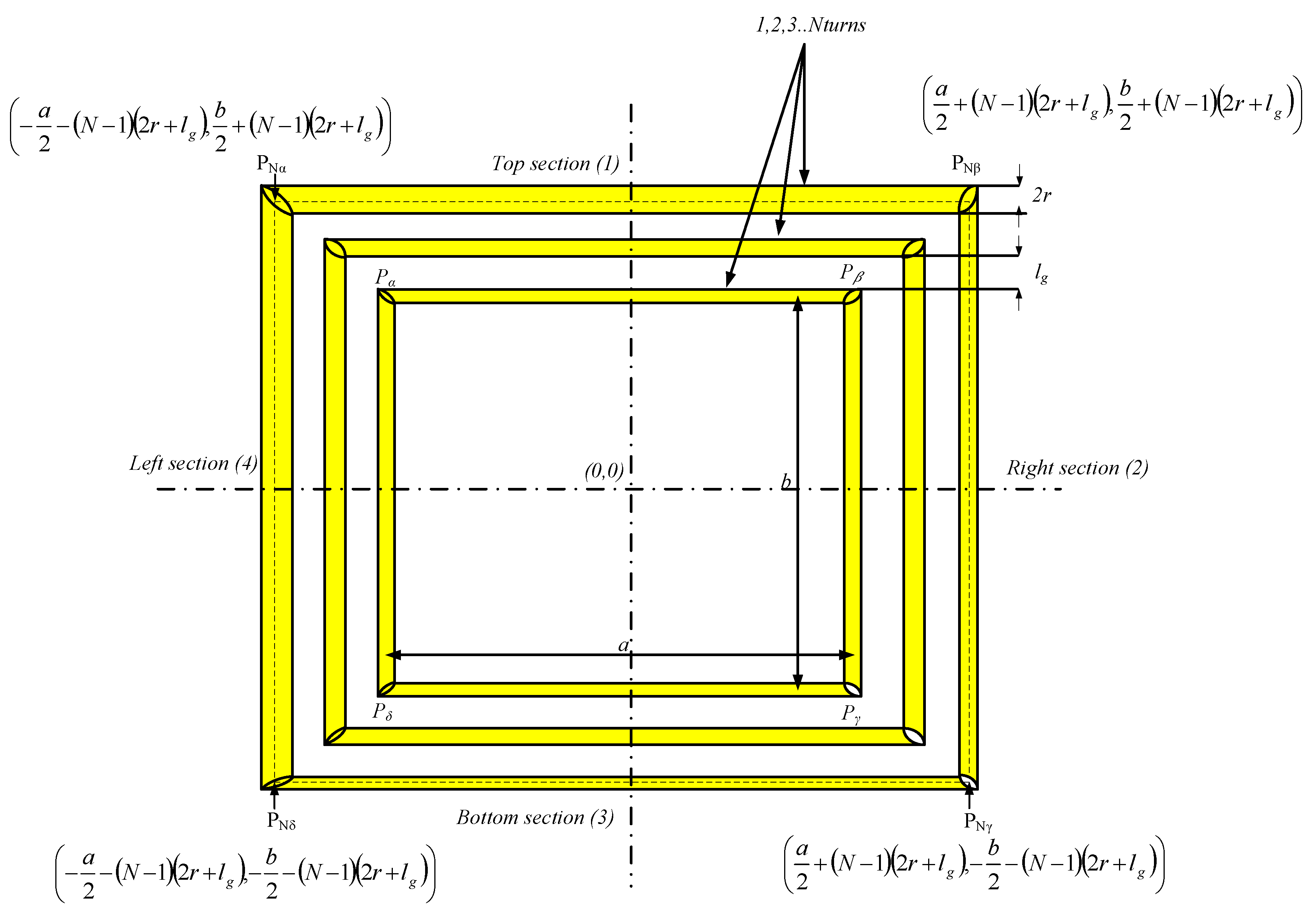
In this paper, we bridge this gap by taking into account the effect of turns (increase of the perimeter for every new turn), as well as any incipient air-gap by using a matrix manipulation. This extends to both single and multi-coil geometries, and their magnetic behavior is analyzed.

2. Neumann’s Integral

The mutual inductance between two current-carrying circuits assuming uniform cross-sectional current density and neglecting radiation can be written in terms of the differential length vector of the two circuits $\overrightarrow{d{l}_1}$, $\overrightarrow{d{l}_2}$ separated by a distance $r_{12}$ in terms of vacuum permeability, ${\mu }_0=4\pi \times {10}^{-7}$ H/m, as:

$$L_{12}=\frac{{\lambda }_2}{i_1}=\frac{{\mu }_0}{4\pi }{\oint }_{c_1}{\oint }_{c_2}\frac{\overrightarrow{d{l}_1}.\overrightarrow{d{l}_2}}{r_{12}}$$

(1)

In Equation (1), contours $c_1$ and $c_2$ are along the middle edge of the circuits 1 and 2 (primary and secondary), respectively. This equation is generic, order independent and can be adapted to model self-inductance by considering the contours $c_1$ and $c_2$ as along the middle edge of the conductor and the inner edge of the wire.

2.1. Circular Coils

In the case of a pair of circular coils, the application of Neumann’s integral as in (1), the two contours $c_1$ and $c_2$ represent the contour of current filaments assumed to be in the middle of the primary and secondary. Now, consider the case of a misaligned circular coil pair, composed of wires of the circular cross-section of radius r and with an air-gap $l_g$ between turns. Such a coil pair is indicated in Figure 1.

Consider $R_p$ and $R_s$ as the radii of the middle contour of the first turn of the primary and secondary. The inner radii of the i-th turn of the primary and the j-th turn of the secondary are related as $R_i=R_p+(i-1)(2r+l_g),R_j=R_s+(j-1)(2r+l_g)$, respectively. In such a case, the partial mutual inductance is written in terms of azimuths, ${\varphi }_i$ and ${\varphi }_j$, of the respective coils as:

$$M_{ij}=\frac{{\mu }_0}{4\pi }\times \left[{\int }_{{\varphi }_i=0}^{2\pi }{\int }_{{\varphi }_j=0}^{2\pi }Id{\varphi }_{i}d{\varphi }_j\right]$$

(2)

where I, $R_i$, $R_j$ are defined as:

$$\begin{array}{c}\hfill I=\frac{R_i{R}_{j}sin{\varphi }_{i}sin{\varphi }_j+R_i{R}_{j}cos{\varphi }_{i}cos{\varphi }_j}{\sqrt{{\left(R_{i}cos{\varphi }_i-(x_0+R_{j}cos{\varphi }_j)\right)}^2+{\left(R_{i}sin{\varphi }_i-(y_0+R_{j}sin{\varphi }_j)\right)}^2}}\end{array}$$

(3)

The final mutual inductance can be defined for the primary having “n” turns and the secondary with “k” turns as:

$$\begin{array}{c}\hfill {\displaystyle M=\sum _{i=1}^n\sum _{j=1}^k{M}_{ij}}\end{array}$$

(4)

The self-inductances can be extracted similarly from (4) by defining the radius of the middle edge and the inner edge of each turn.

2.2. Rectangular Coils

A single turn rectangular coil is shown in Figure 2. A rectangular structure can be split into four sections ($l_{1^{{}^{\prime }}},l_{2^{{}^{\prime }}},..l_{4^{{}^{\prime }}}$), each of which refers to conductors in the top, bottom, left and right, respectively. In such a case, (1) can be written in terms of the various sections of the coil as:

$$L=\frac{{\mu }_0}{4\pi }\times \left[{\oint }_{l_{1^{{}^{\prime }}}}{\oint }_{l_1}\frac{d\overrightarrow{{\mathbf{l}}_{{\mathbf{1}}^{{}^{\prime }}}}·d\overrightarrow{{\mathbf{l}}_{\mathbf{1}}}}{r_{1^{{}^{\prime }}1}}+{\oint }_{l_{2^{{}^{\prime }}}}{\oint }_{l_1}\frac{d\overrightarrow{{\mathbf{l}}_{{\mathbf{2}}^{{}^{\prime }}}}·d\overrightarrow{{\mathbf{l}}_{\mathbf{1}}}}{r_{2^{{}^{\prime }}1}}+{\oint }_{l_{3^{{}^{\prime }}}}{\oint }_{l_1}\frac{d\overrightarrow{{\mathbf{l}}_{{\mathbf{3}}^{{}^{\prime }}}}·d\overrightarrow{{\mathbf{l}}_{\mathbf{1}}}}{r_{3^{{}^{\prime }}1}}+{\oint }_{l_{4^{{}^{\prime }}}}{\oint }_{l_1}\frac{d\overrightarrow{{\mathbf{l}}_{{\mathbf{4}}^{{}^{\prime }}}}·d\overrightarrow{{\mathbf{l}}_{\mathbf{1}}}}{r_{4^{{}^{\prime }}1}}\right]$$

(5)

This can be written as a matrix in the form where the rows represent the section of the conductor that carriers the current (section of the contour of the center), and columns represent the section on which the inductance contribution is considered. Each element of the matrix is a partial inductance (self-partial inductance ($i=j$) and mutual partial inductance ($i\ne j$)).

$$L_{ij}=\frac{{\mu }_0}{4\pi }\times \left[\begin{array}{cccc}{\oint }_{l_{1^{{}^{\prime }}}}{\oint }_{l_1}\frac{d\overrightarrow{{\mathbf{l}}_{{\mathbf{1}}^{{}^{\prime }}}}·d\overrightarrow{{\mathbf{l}}_{\mathbf{1}}}}{r_{1^{{}^{\prime }}1}}& {\oint }_{l_{1^{{}^{\prime }}}}{\oint }_{l_2}\frac{d\overrightarrow{{\mathbf{l}}_{{\mathbf{1}}^{{}^{\prime }}}}·d\overrightarrow{{\mathbf{l}}_{\mathbf{2}}}}{r_{1^{{}^{\prime }}2}}& \cdots & {\oint }_{l_{1^{{}^{\prime }}}}{\oint }_{l_4}\frac{d\overrightarrow{{\mathbf{l}}_{{\mathbf{1}}^{{}^{\prime }}}}·d\overrightarrow{{\mathbf{l}}_{\mathbf{4}}}}{r_{1^{{}^{\prime }}4}}\\ {\oint }_{l_{2^{{}^{\prime }}}}{\oint }_{l_1}\frac{d\overrightarrow{{\mathbf{l}}_{{\mathbf{2}}^{{}^{\prime }}}}·d\overrightarrow{{\mathbf{l}}_{\mathbf{1}}}}{r_{2^{{}^{\prime }}1}}& {\oint }_{l_{2^{{}^{\prime }}}}{\oint }_{l_2}\frac{d\overrightarrow{{\mathbf{l}}_{{\mathbf{2}}^{{}^{\prime }}}}·d\overrightarrow{{\mathbf{l}}_{\mathbf{2}}}}{r_{2^{{}^{\prime }}2}}& \cdots & {\oint }_{l_{2^{{}^{\prime }}}}{\oint }_{l_4}\frac{d\overrightarrow{{\mathbf{l}}_{{\mathbf{2}}^{{}^{\prime }}}}·d\overrightarrow{{\mathbf{l}}_{\mathbf{4}}}}{r_{2^{{}^{\prime }}4}}\\ {\oint }_{l_{3^{{}^{\prime }}}}{\oint }_{l_1}\frac{d\overrightarrow{{\mathbf{l}}_{{\mathbf{3}}^{{}^{\prime }}}}·d\overrightarrow{{\mathbf{l}}_{\mathbf{1}}}}{r_{3^{{}^{\prime }}1}}& {\oint }_{l_{3^{{}^{\prime }}}}{\oint }_{l_2}\frac{d\overrightarrow{{\mathbf{l}}_{{\mathbf{3}}^{{}^{\prime }}}}·d\overrightarrow{{\mathbf{l}}_{\mathbf{2}}}}{r_{3^{{}^{\prime }}2}}& \cdots & {\oint }_{l_{3^{{}^{\prime }}}}{\oint }_{l_4}\frac{d\overrightarrow{{\mathbf{l}}_{{\mathbf{3}}^{{}^{\prime }}}}·d\overrightarrow{{\mathbf{l}}_{\mathbf{4}}}}{r_{3^{{}^{\prime }}4}}\\ {\oint }_{l_{4^{{}^{\prime }}}}{\oint }_{l_1}\frac{d\overrightarrow{{\mathbf{l}}_{{\mathbf{4}}^{{}^{\prime }}}}·d\overrightarrow{{\mathbf{l}}_{\mathbf{1}}}}{r_{4^{{}^{\prime }}1}}& {\oint }_{l_{4^{{}^{\prime }}}}{\oint }_{l_2}\frac{d\overrightarrow{{\mathbf{l}}_{{\mathbf{4}}^{{}^{\prime }}}}·d\overrightarrow{{\mathbf{l}}_{\mathbf{2}}}}{r_{4^{{}^{\prime }}2}}& \cdots & {\oint }_{l_{4^{{}^{\prime }}}}{\oint }_{l_4}\frac{d\overrightarrow{{\mathbf{l}}_{{\mathbf{4}}^{{}^{\prime }}}}·d\overrightarrow{{\mathbf{l}}_{\mathbf{4}}}}{r_{4^{{}^{\prime }}4}}\end{array}\right]$$

(6)

Self-inductance of this rectangular coil can be written as:

$$\begin{array}{c}\hfill {\displaystyle L=\sum _{i=1}^4\sum _{j=1}^4{L}_{ij}}\end{array}$$

(7)

Since the orthogonal terms in the vector dot product reduce to a zero, for example: ($\overrightarrow{d{l}_{1^{{}^{\prime }}}}·\overrightarrow{d{l}_2}=d{x}_1\widehat{i}·dy\widehat{j}=0$).

$$\begin{array}{c}\hfill L=\left[\begin{array}{cccc}{L}_{11}& 0& L_{13}& 0\\ 0& L_{22}& 0& L_{24}\\ L_{31}& 0& L_{33}& 0\\ 0& L_{42}& 0& L_{44}\end{array}\right]\end{array}$$

(8)

Thus, the total external self-inductance can be written in terms of $L_a=L_{11}=L_{33}$, $L_b=L_{22}=L_{44}$, $M_a=L_{13}=L_{31}$, $M_b=L_{24}=L_{42}$ as:

$$\begin{array}{c}\hfill L=2(L_a+L_b-M_a-M_b)\end{array}$$

(9)

where the self-partial inductances $(L_a$, $L_b=L_{(a\leftrightarrow b)})$ are given as an integration of the differential lengths of the inner edge, $d{x}_1$, and middle edge, $d{x}_2$, of the top section as:

$$\begin{array}{c}\hfill L_a=\frac{{\mu }_0}{4\pi }\times \left[{\int }_{-\frac{a}{2}+r}^{\frac{a}{2}-r}d{x}_1{\int }_{-\frac{a}{2}}^{\frac{a}{2}}\frac{d{x}_2}{\sqrt{{(x_2-x_1)}^2+r^2}}\right]\\ \hfill L_a=(a-r)ln\left|\frac{a-r+\sqrt{r^2+{(a-r)}^2}}{-a+r+\sqrt{r^2+{(-a+r)}^2}}\right|+rln\left|\frac{-r+\sqrt{2}r}{r+\sqrt{2}r}\right|\\ \hfill +2\sqrt{2}r-\sqrt{(r^2+{(a-r)}^2)}-\sqrt{(r^2+{(-a+r)}^2)}\end{array}$$

(10)

and the mutual partial inductances $(M_a$, $M_b=M_{(a\leftrightarrow b)})$:

$$M_a=\frac{{\mu }_0}{4\pi }\times \left[{\int }_{-\frac{a}{2}+r}^{\frac{a}{2}-r}d{x}_3{\int }_{-\frac{a}{2}}^{\frac{a}{2}}\frac{d{x}_2}{\sqrt{{(x_2-x_3)}^2+{(b-r)}^2}}\right]$$

(11)

3. Multi-Turn Charge Pads

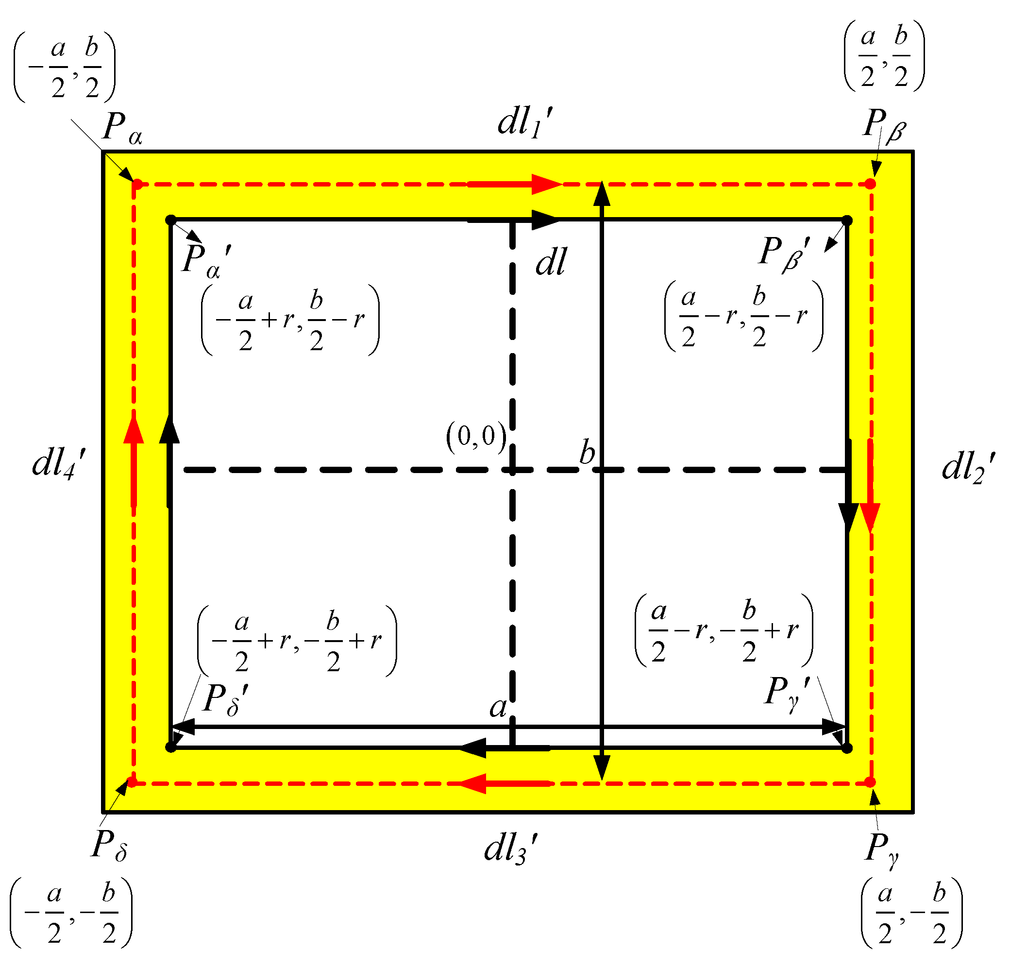
A multi-turn coil is shown in Figure 3. Consider the per-turn inductance written as $L_{ijlk}$, which represents the partial inductance contribution due to current flowing through the i-th turn, j-th section on the l-th turn, k-th section. In such a case, it is important to derive the expressions of the mutual partial inductances considering that the dimensions of the coil change with corresponding change in the number of turns. It is useful to list the vertices of the extremes of the contour along the center of the wire, as well as along the inner edge of the wire for the N-th winding.

The partial self-inductance of the N-th turn (due to the first section) can be derived as:

$$L_{N1N1}=\frac{{\mu }_0}{4\pi }\times \left[{\int }_{k_1}^{k_2}d{x}_1{\int }_{\alpha }^{\beta }\frac{d{x}_2}{\sqrt{{(x_2-x_1)}^2+r^2}}\right]$$

(12)

where,

$$\begin{array}{c}\hfill k_1=\left(-\frac{a}{2}+r\right)-(N-1)(2r+l_g),k_2=\left(\frac{a}{2}-r\right)+(N-1)(2r+l_g)\\ \hfill \alpha =-\frac{a}{2}-(N-1)(2r+l_g),\beta =\frac{a}{2}+(N-1)(2r+l_g)\end{array}$$

(13)

The result of such an integration is:

$$\frac{{\mu }_0}{4\pi }\times \left[I(C=\beta )-I(C=\alpha )\right]$$

(14)

where,

$$I\left(C\right)=\sqrt{r^2+{\left(C-k_2\right)}^2}-\sqrt{r^2+{\left(C-k_1\right)}^2}+ln\left|\frac{{\left(\sqrt{r^2+{\left(C-k_1\right)}^2}+\left(C-k_1\right)\right)}^{\left(C-k_1\right)}}{{\left(\sqrt{r^2+{\left(C-k_2\right)}^2}+\left(C-k_2\right)\right)}^{\left(C-k_2\right)}}\right|$$

(15)

The self-inductance matrix can be written as:

$$L_{ijlk}=\frac{{\mu }_0}{4\pi }\times \left[\begin{array}{cccc}{\displaystyle \sum _{i=1}^N\sum _{l=1}^N{L}_{i1l1}}& 0& {\displaystyle -\sum _{i=1}^N{\displaystyle \sum _{l=1}^N{L}_{i1l3}}}& 0\\ 0& {\displaystyle \sum _{i=1}^N\sum _{l=1}^N{L}_{i2l2}}& 0& -{\displaystyle \sum _{i=1}^N\sum _{l=1}^N{L}_{i2l4}}\\ {\displaystyle -\sum _{i=1}^N\sum _{l=1}^N{L}_{i3l1}}& 0& {\displaystyle \sum _{i=1}^N\sum _{l=1}^N{L}_{i3l3}}& 0\\ 0& {\displaystyle -\sum _{i=1}^N\sum _{l=1}^N{L}_{i4l2}}& 0& {\displaystyle \sum _{i=1}^N\sum _{l=1}^N{L}_{i4l4}}\end{array}\right]$$

(16)

The diagonal terms in the above matrix are the sectional partial self-inductance, and the off-diagonal terms are the sectional partial mutual inductance. Note that the signs of sectional self-inductance are positive, and those of the sectional partial mutual inductance are negative for rectangular structures. The summation terms can be evaluated by calculating some general matrices like $L_{N1k1},L_{N1k3}$. The inductance contributions of $L_{N2k2},L_{N2k4}$ can be obtained by inverting $a\leftrightarrow b$ in the previous set of general expressions. The net self-inductance can then be written as:

$${\displaystyle L=\sum _{i=1}^N\sum _{j=1}^4\sum _{l=1}^N\sum _{k=1}^4{L}_{ijlk}}$$

(17)

Sectional Partial Inductances

The sectional partial self-inductance is defined as the sum of the partial self- and partial mutual inductance contributions of current in a particular section on the same section on all possible turns. The sectional partial mutual self-inductance is defined as the sum of the partial mutual inductance contributions of the current in a particular section on a different section for all combinations of possible turns. Following the previous procedures, the partial self-inductance due to current in the N-th turn first section on the k-th turn first section is given by:

$$\begin{array}{c}\hfill L_{N1k1}=\frac{{\mu }_0}{4\pi }\times \left[{\int }_{k_1}^{k_2}d{x}_1{\int }_{\alpha }^{\beta }\frac{d{x}_2}{\sqrt{{(x_2-x_1)}^2+{\left(r+(N-k)(2r+l_g)\right)}^2}}\right]\\ \hfill \mathrm{Symbols}:k_1=\left(-\frac{a}{2}+r\right)-(k-1)(2r+l_g),k_2=\left(\frac{a}{2}-r\right)+(k-1)(2r+l_g)\\ \hfill \alpha =-\frac{a}{2}-(N-1)(2r+l_g),\beta =\frac{a}{2}+(N-1)(2r+l_g)\end{array}$$

(18)

The result of this integration is the same as (14) with $I\left(C\right)$ defined as:

$$\begin{array}{c}\hfill I\left(C\right)=\sqrt{{(r+(N-k)(2r+l_g))}^2+{\left(C-k_2\right)}^2}\\ \hfill -\sqrt{{(r+(N-k)(2r+l_g))}^2+{\left(C-k_1\right)}^2}\\ \hfill +ln\left|\frac{{\left(\sqrt{{(r+(N-k)(2r+l_g))}^2+{\left(C-k_1\right)}^2}+\left(C-k_1\right)\right)}^{\left(C-k_1\right)}}{{\left(\sqrt{{(r+(N-k)(2r+l_g))}^2+{\left(C-k_2\right)}^2}+\left(C-k_2\right)\right)}^{\left(C-k_2\right)}}\right|\end{array}$$

(19)

Similarly, the partial mutual self-inductance can be written as:

$$\begin{array}{c}\hfill L_{N1k3}=\frac{{\mu }_0}{4\pi }\times \left[{\int }_{k_1}^{k_2}d{x}_1{\int }_{\alpha }^{\beta }\frac{d{x}_2}{\sqrt{{(x_2-x_1)}^2+{\left((b-r)+(2r+l_g)(N+k-2)\right)}^2}}\right]\\ \hfill \mathrm{Symbols}:\\ \hfill k_1=\left(-\frac{a}{2}+r\right)-(k-1)(2r+l_g),k_2=\left(\frac{a}{2}-r\right)+(k-1)(2r+l_g)\\ \hfill \alpha =-\frac{a}{2}-(N-1)(2r+l_g),\beta =\frac{a}{2}+(N-1)(2r+l_g)\end{array}$$

(20)

Again, the result of this integration is the same as (14) with $I\left(C\right)$ defined as:

$$\begin{array}{c}\hfill I\left(C\right)=\sqrt{({(N+k-2)(2r+l_g)+\left(b-r\right))}^2+{\left(C-k_2\right)}^2}\\ \hfill -\sqrt{{((N+k-2)(2r+l_g)+(b-r))}^2+{\left(C-k_1\right)}^2}\\ \hfill +ln\left|\frac{{\left(\sqrt{{((N+k-2)(2r+l_g)+(b-r))}^2+{\left(C-k_1\right)}^2}+\left(C-k_1\right)\right)}^{\left(C-k_1\right)}}{{\left(\sqrt{{((N+k-2)(2r+l_g)+(b-r))}^2+{\left(C-k_2\right)}^2}+\left(C-k_2\right)\right)}^{\left(C-k_2\right)}}\right|\end{array}$$

(21)

4. Mutual Inductance between Rectangular Coils

A simple description of the mutual inductance scenario of a single turn primary and a single turn secondary is depicted in Figure 4. As an extension of the theory previously developed, the mutual inductance for a multi-turn rectangular coil can be written in terms of the contributions due to current flowing through the i-th turn, j-th section of the primary on the l-th turn, k-th section on the secondary. The sectional mutual inductance matrix can be written as:

$$\begin{array}{c}\hfill M_{ijlk}=\frac{{\mu }_0}{4\pi }\times \left[\begin{array}{cccc}{\displaystyle \sum _{i=1}^N\sum _{l=1}^N{M}_{i1l1}}& 0& {\displaystyle -\sum _{i=1}^N{\displaystyle \sum _{l=1}^N{M}_{i1l3}}}& 0\\ 0& {\displaystyle \sum _{i=1}^N\sum _{l=1}^N{M}_{i2l2}}& 0& -{\displaystyle \sum _{i=1}^N\sum _{l=1}^N{M}_{i2l4}}\\ {\displaystyle -\sum _{i=1}^N\sum _{l=1}^N{M}_{i3l1}}& 0& {\displaystyle \sum _{i=1}^N\sum _{l=1}^N{M}_{i3l3}}& 0\\ 0& {\displaystyle -\sum _{i=1}^N\sum _{l=1}^N{M}_{i4l2}}& 0& {\displaystyle \sum _{i=1}^N\sum _{l=1}^N{M}_{i4l4}}\end{array}\right]\end{array}$$

(22)

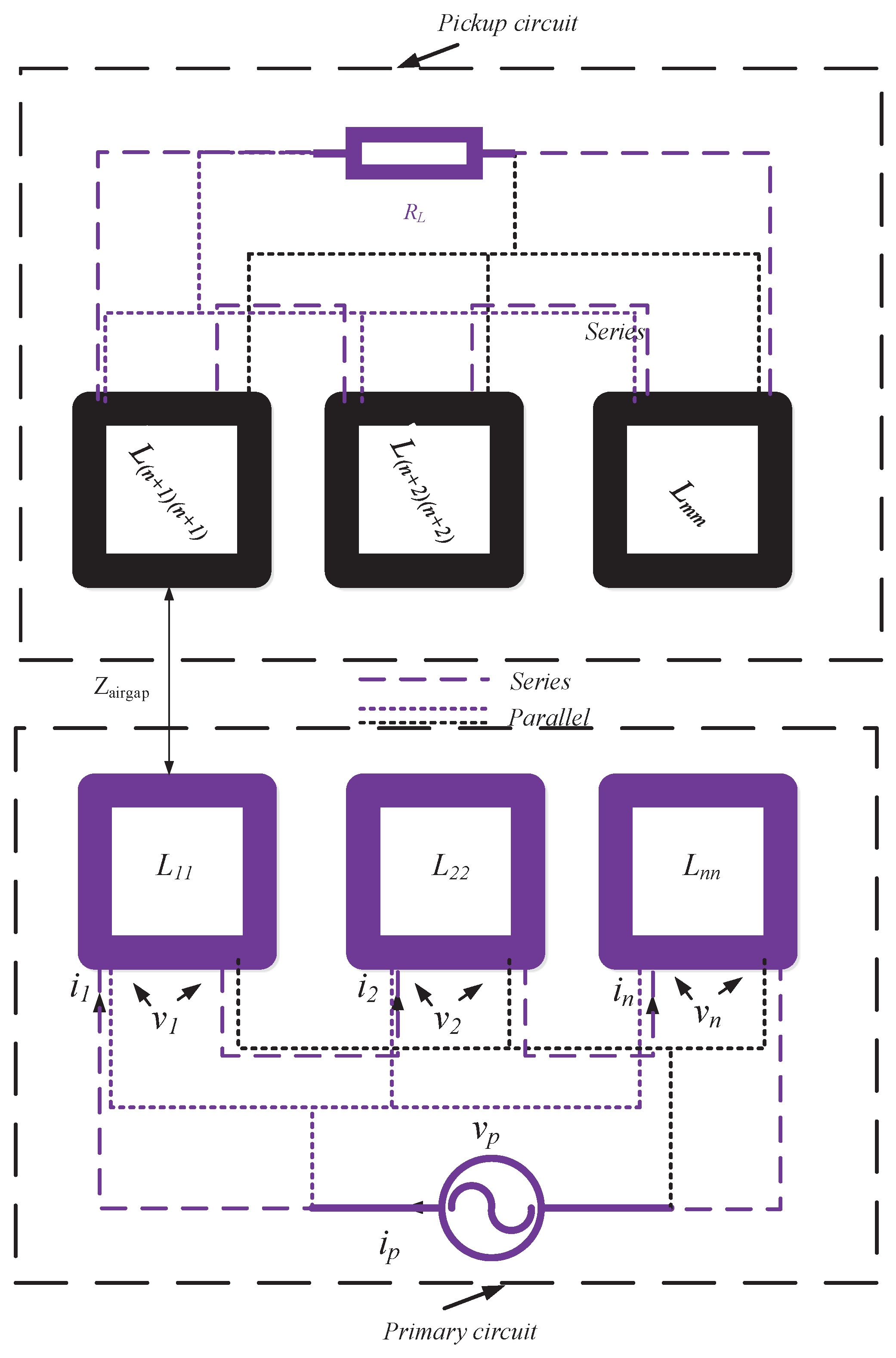
5. Extension to Multi-Coil Charge Pad (MCCP)

Consider a linear magnetic system excited by a pure sinusoidal (non-harmonic) voltage consisting of a primary and a pickup composed of several segmented coils as shown in Figure 5. The coils can be individually connected serially or in parallel to compose the multi-coil charge-pad. Let the primary be composed of “n” coils, $(1,2,..n)$ and the pickup with “$m-n$” coils, $(n+1,n+2,..m,$ $(m>n))$. Consequently, the voltage matrix, $\left[\begin{array}{c}V\end{array}\right]$ for all of the coils can be written in terms of currents, $\left[\begin{array}{c}i\end{array}\right]$, and time-derivative of currents, $\left[\begin{array}{c}\frac{di}{dt}\end{array}\right]$:

$$\begin{array}{c}\hfill \left[\begin{array}{c}V\end{array}\right]=\left[\begin{array}{c}L\end{array}\right]\times \left[\begin{array}{c}\frac{di}{dt}\end{array}\right]+\left[\begin{array}{c}R\end{array}\right]\times \left[\begin{array}{c}i\end{array}\right]\end{array}$$

(23)

where the matrices are defined as:

$$\begin{array}{c}\hfill \left[V\right]=\left[\begin{array}{c}{v}_1\\ v_2\\ ⋮\\ v_n\\ v_{n+1}\\ v_{n+2}\\ ⋮\\ v_m\end{array}\right]\left[\frac{di}{dt}\right]=\left[i^{\prime }\right]=\left[\begin{array}{c}{i}_1^{\prime }\\ i_2^{\prime }\\ ⋮\\ i_n^{\prime }\\ i_{n+1}^{\prime }\\ i_{n+2}^{\prime }\\ ⋮\\ i_m^{\prime }\end{array}\right]\left[i\right]=\left[\begin{array}{c}{i}_1\\ i_2\\ ⋮\\ i_n\\ i_{n+1}\\ i_{n+2}\\ ⋮\\ i_m\end{array}\right]\left[R\right]=\left[\begin{array}{cccccccc}{R}_1& 0& 0& 0& 0& 0& 0& 0\\ 0& R_2& 0& 0& 0& 0& 0& 0\\ ⋮& ⋮& ⋮& ⋮& ⋮& ⋮& ⋮& ⋮\\ 0& 0& 0& 0& 0& 0& 0& R_8\end{array}\right]\end{array}$$

(24)

Finally, $\left[L\right]$ is defined as:

$$\begin{array}{c}\hfill \left[L\right]=\left[\begin{array}{cccccccc}{L}_{11}& L_{12}& \cdots & L_{1n}& L_{1(n+1)}& L_{1(n+2)}& \cdots & L_{1\left(m\right)}\\ L_{21}& L_{22}& \cdots & L_{2n}& L_{2(n+1)}& L_{2(n+2)}& \cdots & L_{2\left(m\right)}\\ ⋮& ⋮& ⋮& ⋮& ⋮& ⋮& ⋮& ⋮\\ L_{n1}& L_{n2}& \cdots & L_{nn}& L_{n(n+1)}& L_{n(n+2)}& \cdots & L_{n\left(m\right)}\\ L_{(n+1)1}& L_{(n+1)2}& \cdots & L_{(n+1)n}& 0& 0& 0& 0\\ L_{(n+2)1}& L_{(n+2)2}& \cdots & L_{(n+2)n}& 0& 0& 0& 0\\ ⋮& ⋮& ⋮& ⋮& 0& 0& 0& 0\\ L_{m1}& L_{m2}& \cdots & L_{mn}& 0& 0& 0& 0\end{array}\right]\end{array}$$

(25)

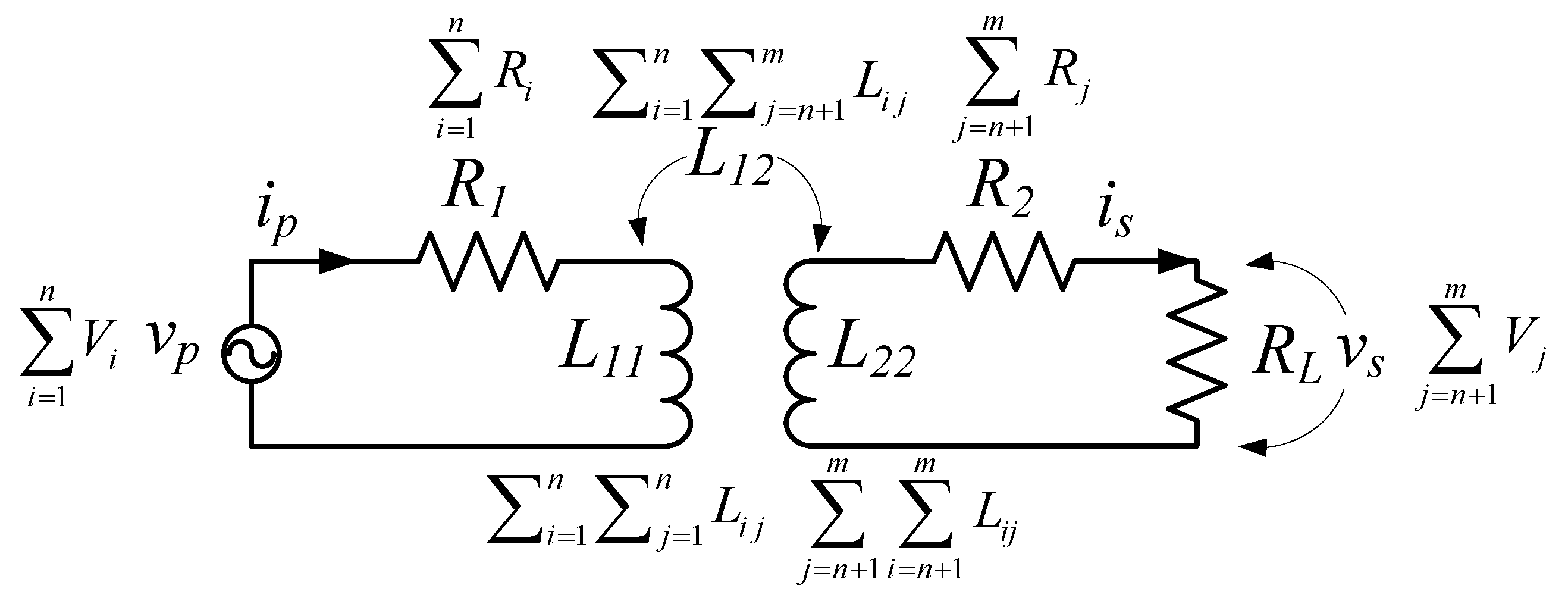
The series and parallel combination can now be decomposed from this multi-coil combination. In the case of a series connected set of coils, $i_p=i_1=i_2\cdots =i_n$ and $i_s=i_{n+1}=i_{n+2}\cdots =i_m$. Furthermore, in the case of the parallel set of coils, $i_p=i_1+i_2\cdots +i_n$ and $i_s=i_{n+1}+i_{n+2}\cdots +i_m$. After such a transformation, it becomes easy to reduce such a system of parallel or series coils into a single coil-pair. In such a system, for both the series and parallel system of coils, it can be easy to prove that:

$$\begin{array}{c}\hfill \left[\begin{array}{c}{\displaystyle \sum _{i=1}^n{v}_i}\\ {\displaystyle \sum _{j=n+1}^m{v}_j}\end{array}\right]=\left[\begin{array}{cc}{\displaystyle \sum _{i=1}^n\sum _{j=1}^n{L}_{ij}}& {\displaystyle \sum _{i=1}^n\sum _{j=n+1}^m{L}_{ij}}\\ {\displaystyle \sum _{j=n+1}^m\sum _{i=1}^n{L}_{ij}}& {\displaystyle \sum _{j=n+1}^m\sum _{i=n+1}^m{L}_{ij}}\end{array}\right]\times \left[\begin{array}{c}{i_p}^{\prime }\\ {i_s}^{\prime }\end{array}\right]+\left[\begin{array}{cc}{\displaystyle \sum _{i=1}^n{R}_i}& 0\\ 0& {\displaystyle \sum _{j=n+1}^m{R}_j}\end{array}\right]\times \left[\begin{array}{c}{i}_p\\ i_s\end{array}\right]\end{array}$$

(26)

Equation (26) indicates that it is possible to convert a linear magnetic system with multi-coils into a system of a single coil pair by calculating the individual contributions. Such an equivalent coil system is shown in Figure 6. Such a transposition makes it easy to analytically model multi-coil linear magnetic systems by using the principles of single coils already developed previously.

6. Validation of Analytical Model

To validate the analytical models that are developed in the previous sections, finite element method (FEM) simulation and experimentation are carried out. Circular and rectangular shapes are compared. The physical properties of the coils are tabulated in

Table 1. Properties of the compared circular and rectangular coils.

Type of Coil	a (cm)	b (cm)	l${}_{\mathit{g}}$ (cm)	N (turns)
Rectangular $\left(R1\right)$	4	2	$0.6$	9
Rectangular $\left(R2\right)$	6	4	$0.6$	15
Circular $\left(C\right)$	inner diameter = $5.5$ cm			14
Litz wire used	$600\times 0.071$ mm, 2.1 mm dia overall

. To show the efficacy of analytical expressions, a reduced fill factor was employed for rectangular coils by maintaining an air-gap of $0.6$ cm between the turns.

The constructed coils are shown in Figure 7. The measurements, analysis and simulations are carried out at variable z-gaps between the coils and also at several misaligned positions. The z-gaps are simulated at 3, 5, 7 and 9 cm of coil displacements in the z-direction, taking vertical misalignment into consideration. In the case of lateral misalignment, perfect alignment, $75\%$, $50\%$ and $25\%$ alignments are chosen along the x-axis. The results along the y-axis for symmetrical shapes follows the same trend as the x-axis and, hence, not considered.

Measurements are made by using the Agilent 4294A impedance analyzer (Agilent Technologies, Santa Clara, CA, USA) with the frequency set to 85 kHz. The mutual inductances are extracted from self-inductances by carrying out a constructive and destructive flux measurement by connecting the coils serially from one end to the other and then swapping one of the ends ($L_{const}$, $L_{des}$). The expressions used for extracting the mutual inductance and coupling are:

$$\begin{array}{c}\hfill M=\frac{L_{const}-L_{des}}{4}\\ \hfill k=\frac{M}{\sqrt{L_1{L}_2}}\end{array}$$

(27)

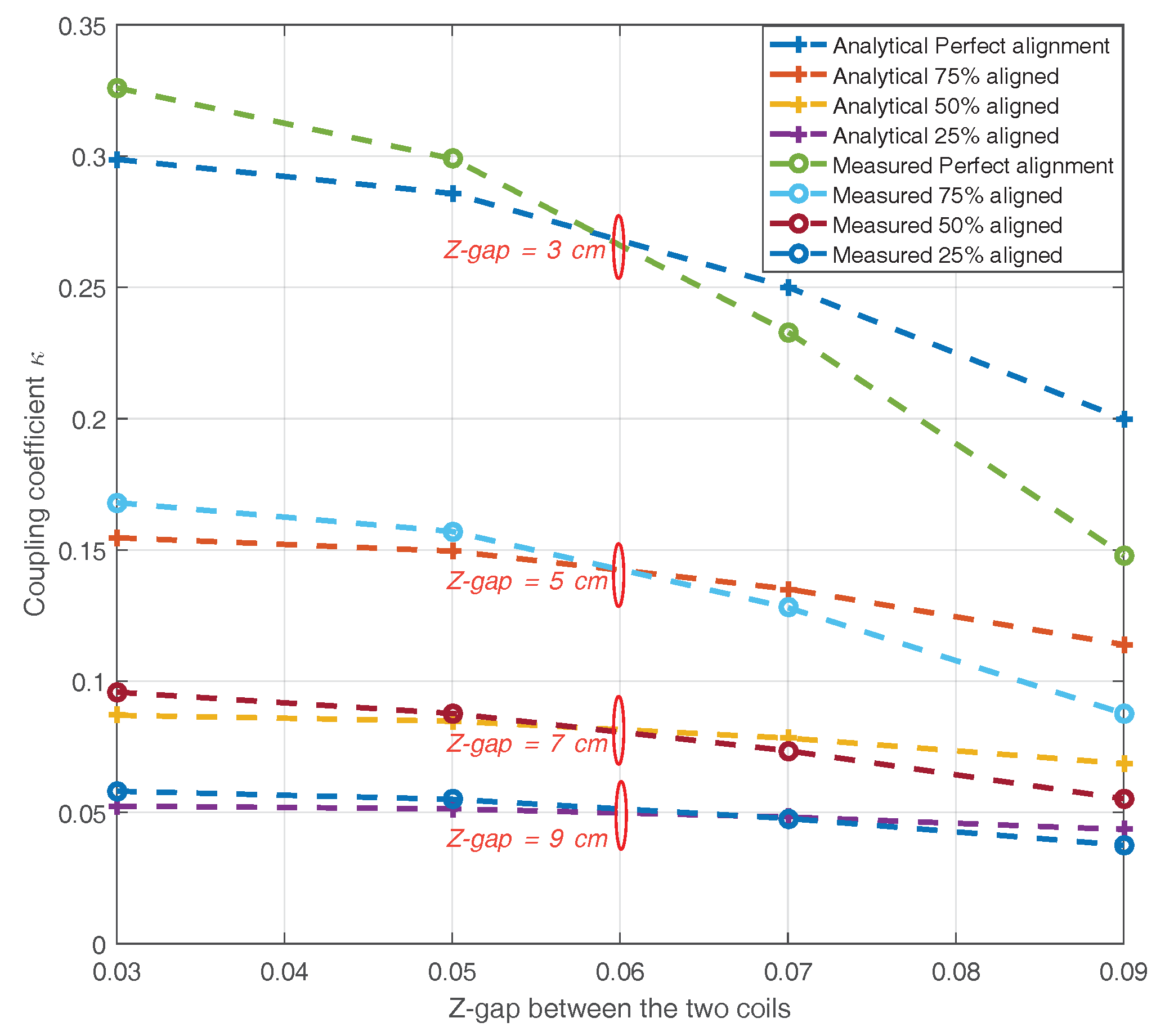
The analytical expressions for circular coils are calculated from Equations (1)–(4). Furthermore, for rectangular coils, Equations (12)–(22) are computed. MATLAB scripts are written separately for each of the computations, and a software tool for self-, mutual and coupling computations is developed for air-cored coils. A comparison of coupling obtained analytically and by making measurements for circular coils is presented in Figure 8. The results show a large degree of agreement between the analytical expressions and the measured results. Mismatches in the results are due to the use of the litz wire in the experiments (unlike a solid conductor used in the analysis) and eddy currents (proximity effects) in the coils that are not considered in the analytical expressions. Some instrumental accuracy limitations also add to this error. However, most observations are within $1\%$ accuracy except for an odd set in the neighborhood of $6\%$. These accuracy measures are acceptable for magnetic analysis.

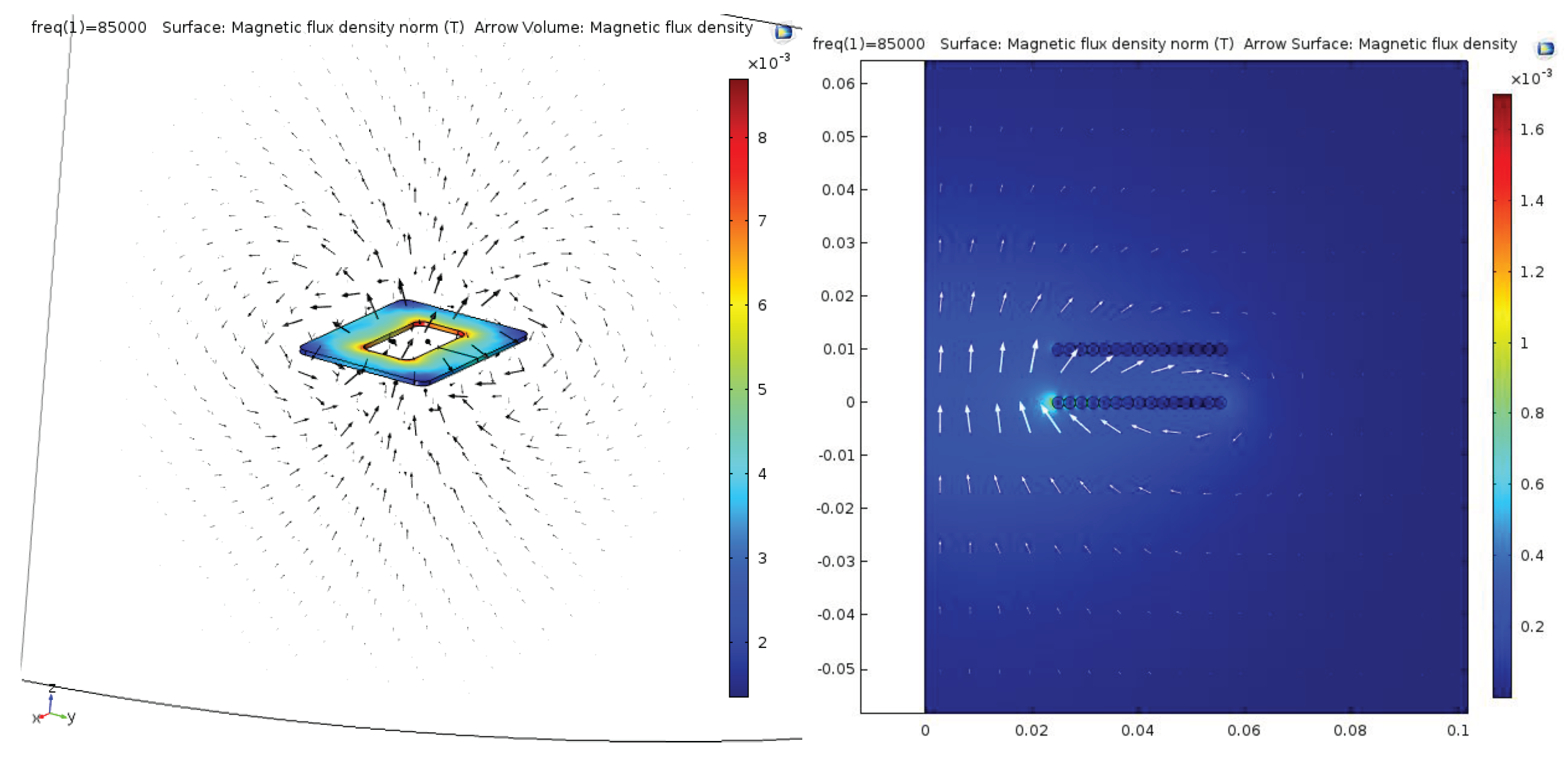
FEM models were created and simulated so as to perform the numerical evaluation of the coils considered. The FEM models developed using COMSOL Multiphysics 5.1 are presented in Figure 9.

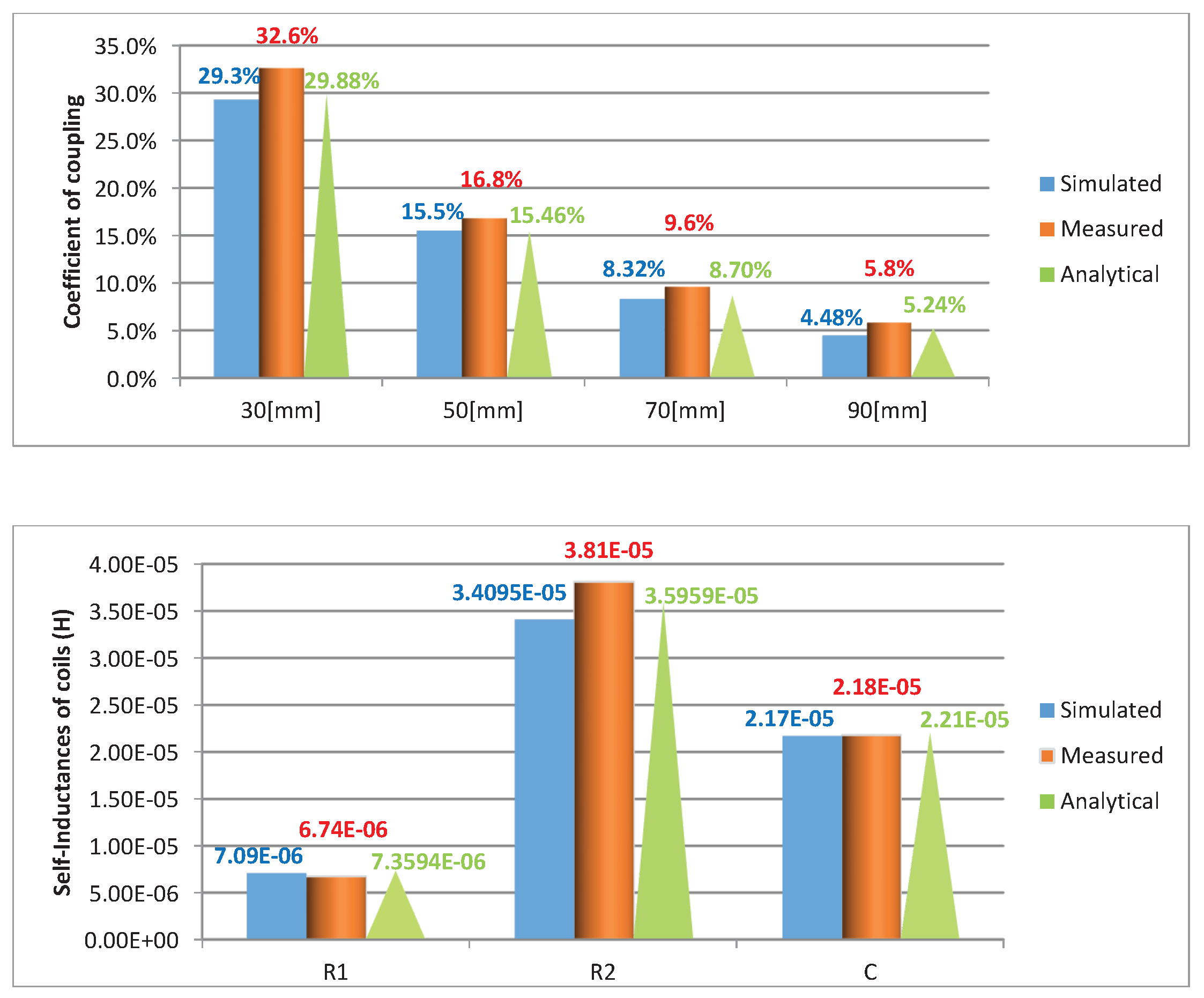
The coupling and self-inductances of circular and rectangular coils are compared analytically, using FEM simulations and experimentation. The results are presented in Figure 10, the coupling being recorded at perfect alignment and variable z-gaps, while self-inductances measured for all variable shapes. All measurements show the same trend, and there is a close match between analytical observations, FEM simulations and measurements.

7. Shape and Performance of Air Couplers

The effect of shapes in IPT systems can be analyzed for air-cored couplers based on the mathematical analysis that has been derived previously. To make such a comparison, a few performance parameters are considered. They are the open circuit voltage $v_{oc}$, short circuit current $i_{sc}$, uncompensated power, $s_{uncomp}$, and maximum efficiency, ${\eta }_{max}$. Open circuit voltage is the maximum voltage that the IPT system can source, and short circuit current is the maximum current that the same can deliver.

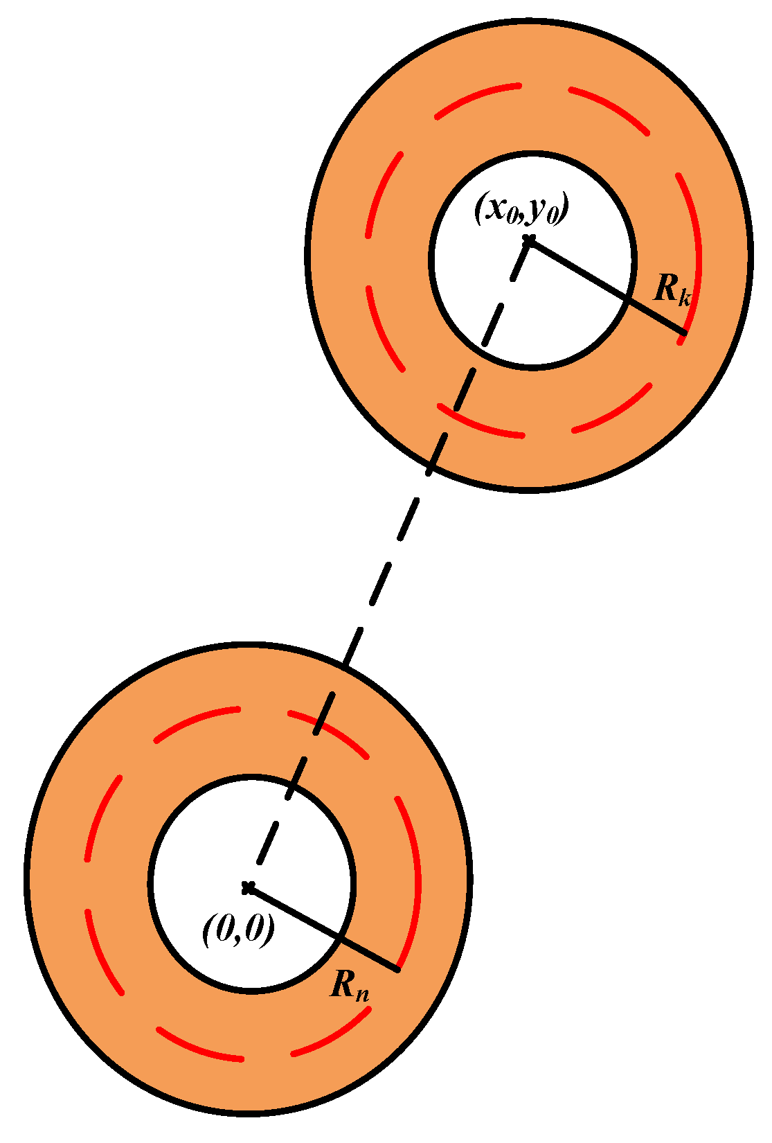
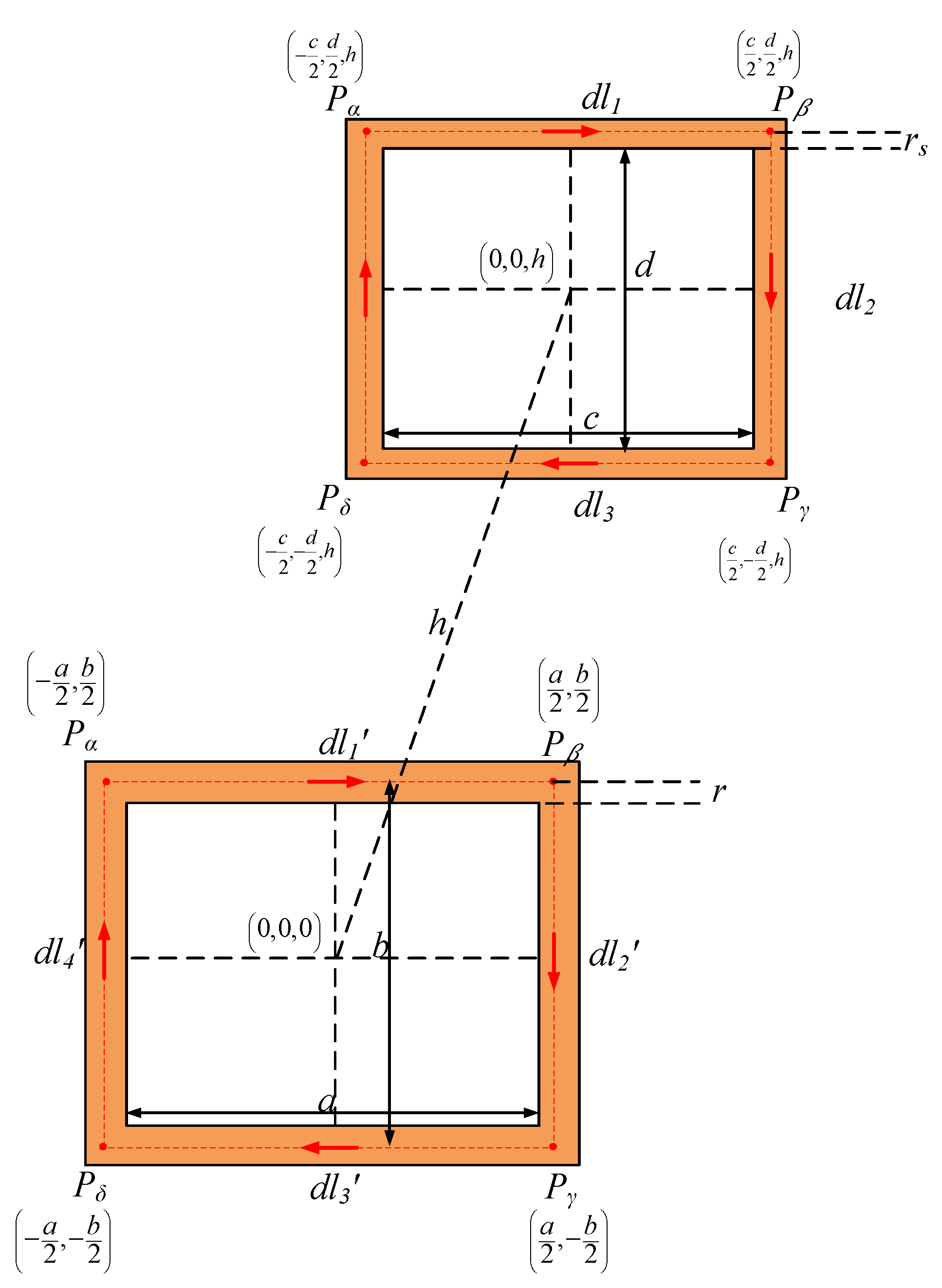
For a coupled charge-pad, if $L_1$ and $L_2$ are the self-inductances of the two couplers with “M” as the mutual inductance and operated at angular frequency $\omega$, creating current $i_1$ through the primary, the open-circuit voltage is defined as $v_{oc}=j\omega M{i}_1$, and during the short-circuit, if $i_{sc}$ is the current flowing in the pickup, $i_{sc}={\displaystyle \frac{v_{oc}}{j\omega L_2}}={\displaystyle \frac{M{i}_1}{L_2}}$. Now, load independent uncompensated reactive power VA is defined as:

$$\begin{array}{c}\hfill s_{uncomp}=v_{oc}\times i_{sc}=\frac{\left(i_1^2{M}^2\omega \right)}{L_2}\end{array}$$

(28)

For the sake of completeness, the output real power for a primary and secondary compensated system is defined in terms of loaded quality factor of the pickup, $Q_{2L}=(\omega \times L_2)/(R_L+R_2)$, where $R_L$ is the load resistance and $R_2$ is the AC resistance of the pickup charge-pad as:

$$\begin{array}{c}\hfill P_{out}=v_{oc}\times i_{sc}\times Q_{(2,L)}=\frac{\left(i_1^2{M}^2{Q}_{(2,L)}\omega \right)}{L_2}\end{array}$$

(29)

The load independent uncompensated VA of the pickup is used further in this paper (28). Furthermore, the maximum efficiency of IPT systems has been derived independent of compensation applied and load present in terms of native quality factors of the primary $\left(Q_1\right)$ and pickup $\left(Q_2\right)$ as [11]:

$${\eta }_{max}=\frac{k\sqrt{Q_1{Q}_2}}{2+k\sqrt{Q_1{Q}_2}}$$

(30)

These parameters have been used to compare a number of differently-shaped air-cored charge-pads. All shapes considered have been analyzed keeping area conserved. This way, generalizations of the behavior of fields and, hence, coupling, power transferred and other parameters are possible. Several analyses were also carried out keeping the perimeter conserved and multi-turns with similar results. In addition, these results also correspond and can be generalized to charge-pads with flux-enhancing materials such as ferrite. This enhanced coupling is obtained by placing ferrites along the natural direction of flux lines. Hence, the basic tendency of the shape in terms of coupling and its gradient is similar in all IPT applications. The compared shapes are listed in

Table 2. Physical parameters of various coil shapes used in the air-cored coupler.

Considered Shape	Parameters	Self-Inductances H
Rectangle dimension	650 & 400 mm	$2.28\times {10}^{-6}$
Square dimension	$509.9$ & $509.9$ mm	$2.23\times {10}^{-6}$
Circle radius	$287.6$ mm	$2.07\times {10}^{-6}$
Double circle (DC) dimension	$203.4$ mm	$2.95\times {10}^{-6}$
Double rectangle (DR) symmetric dimension	$459.6$ & $282.8$ mm	$2.9\times {10}^{-6}$
Double rectangle + quadrature symmetric dimension (DR + Q)	$375.3$ & $230.9$ mm	$2.26\times {10}^{-6}$ (DR) & $1.18\times {10}^{-6}$ (Q)
Area	0.2600 (m${}^2$)

. All considered shapes have been simulated with a one turn coil and a z-gap of 1 cm. This so that the effects of shapes are more enhanced.

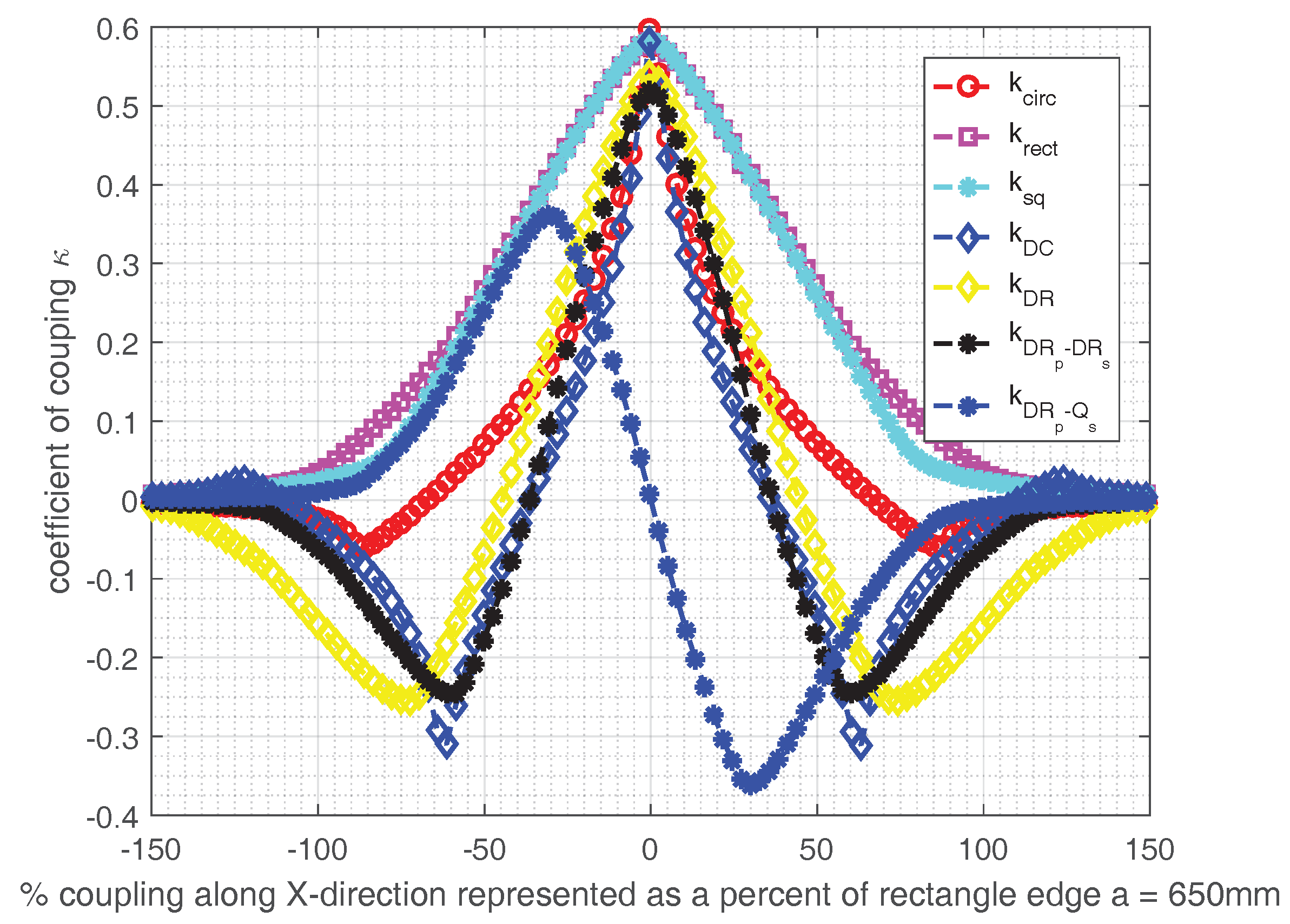
The multi-coil shapes are composed of multiple symmetric coils that are placed close to each other with the coils carrying currents in the opposite direction. The mutual inductance and coupling of these charge-pads are obtained by analyzing (26) and using the mathematical analysis of single coils. A study of coupling by misaligning the coils along x-direction (lateral displacement) is presented in Figure 11.

It can be inferred that circle and four-sided shapes differ in the tolerance to coupling variations when subjected to lateral misalignment. The coupling of rectangular and square coils tends to decay gradually, while the circular shape sees a sharper drop with misalignment. The circular shape, due to the fact that it has the highest area for a given perimeter among closed shapes, has the highest coupling at the best aligned point. The double coils also share the same feature, but with a larger extension of the power profile. It is important to note that in this analysis, since the area is kept conserved, the perimeter varies between the shapes, and hence, it is important to keep trends in mind, rather than absolute values. Null-coupling points in double rectangle (DR) and double circle (DC) coils occur at positions where a pick-up coil is confronted with opposing flux of equal magnitude from the primary charge-pad. Among the double coils, the DC geometry has greater best-aligned coupling than that of DR geometry. However, the misalignment profile for DR coils is broader than that of DC coils, and hence, it is well suited to applications where larger misalignment behavior is expected, for example EVs. When such an analysis was broadened to include the behavior of a DR primary and a DRQ (DR+Q) pick-up, the Q picking up flux emanating from a DR primary behaves best at the misaligned points, while the worst at the best-aligned point. On the contrary, the DR pick-up behaves complementary to the Q pick-up with a DR primary.

Power transferred to the pick-up is evaluated from Equation (28). The uncompensated power calculated when subjected to lateral misalignment is shown in Figure 12. Among single coils, the circular coil has a sharp misalignment band, while the four-sided shapes have greater tolerance. The double shapes follow the features of their single equivalents, with the difference that there is a misalignment point when a single coil among both the primary and pick-up receives power. This creates two more zones of power transfer apart from the best aligned point. In these points, the power is reduced to $<25\%$ as the pick-up voltage is reduced to half, which in turn halves the pick-up current. However, these double shapes suffer from a no-power zone created at the null coupling points. These null power points can be eliminated by using a quadrature coil, the coupling of which is complementary to the main coils, and hence, an addition of power from the quadrature coils removes these null zones. It is important to note that in an actual implementation, the magnitudes of these curves will depend on the number of turns of each coil, the materials present, the source characteristic-voltage/current, resonant behavior, etc.

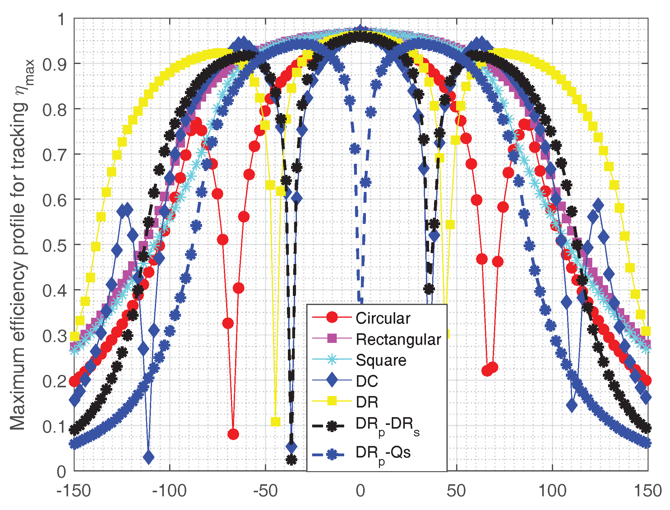
The maximum efficiency as presented in Equation (30) has a dependence on the quality factor, which in turn depends on the AC resistances of the coils. The AC resistances for the litz wire used are extracted from a tabulation technique as presented in [12]. The calculated AC resistance factor including both skin and proximity effects for the litz wire indicated in Table 1 is ${\displaystyle \frac{R_{ac}}{R_{dc}}}=1.029$. The result of maximum efficiency computation when subjected to variable coupling during misalignment is shown in Figure 13. This plot represents the theoretical maximum efficiency that can be expected at various misaligned points for various shapes. The efficiency values floor at the power null points as expected.

8. Discussion

In this paper, a generic analytical tool that is useful to model the magnetics of single and multi coil geometries is developed. The analytical equations developed can be extended to polygonal shapes and can be used to model n-multi-coil geometries, as well. The analytical expressions have the strength that they are computationally efficient, e.g., the computation of inductances and coupling of a single turn rectangular charge-pad take 0.653 s (2.2-GHz Intel i3-processor and 4 GB RAM). In the case of FEM analysis, each individual calculation takes several seconds. This difference gets exaggerated for multi-coil IPT systems, and the analytical formulation yields accurate and fast results.

Such an analytical approach can yield the variation in magnetic parameters due to coupler geometry. Now, different applications of IPT systems can have different objectives: minimization of gradient of coupling in highly misalignment-tolerant EV IPT systems $min(\frac{\partial k}{\partial x},\frac{\partial k}{\partial y})$; elimination of power null points in power-sensitive applications $(P_{x,y}\ne 0)$. Thus, different strategies can be evolved based on the spatial variation of coupling, efficiency and/or power transfer. This paper can empower this decision making before going in for a detailed multi-objective optimization after fixing a geometry suited to the application.

However, a limitation that this approach has is that the principle of superposition holds for linear magnetic systems. Thus, non-linearities in the system such as saturation are neglected in the study. This is a valid assumption for air-cored geometries, and hence, the study yields good results. However, interfaces of different materials in high power IPT systems, such as ferrites and shielding materials (aluminum), need to respect boundary conditions to compute magnetic parameters. Thus, the equations need to be adapted for boundaries, and this extension is beyond the scope of this paper. In related work, an analytical LCL filter design where interfaces are modeled by using the method of images is presented in [13]. The image method can be applied to the analysis in this paper to model the parameters of couplers with several material interfaces. Additionally, the effect of frequency on inductances (due to eddy currents) is not considered in this paper.

A detailed numerical optimization based on the inputs from this study so as to optimize ferrite, aluminum and other materials that may be present in charge-pads is the next step. Such an FEM optimization for a 1-kW DR system is presented in [14]. Some useful results obtained from the analysis are:

• The analysis, compared with FEM and experiments, has a good match. Almost all observations have an error less than $10\%$. This is acceptable for magnetic analysis.
• The coupling of single coils is such that circular coils have the best coupling at the well-aligned point, and the four shapes of coils have a larger misalignment-tolerant band. Thus, rectangular coils can be used for more misalignment-tolerant designs and circular for well-aligned applications.
• The coupling behavior of multi-coil geometries follows the trend of single-coil shapes, but having null-coupling points. By designing a Q coil located between the mid-points of the single coils, flux can be captured at the null-coupling points.
• The Q and DR pickup have complementary coupling-misalignment behavior. At the best aligned point, the Q picks up no flux, and at the misalignment point of null-coupling of the DR pickup, the Q picks up the maximum flux.
• The DR and DC shapes can effectively extend the range of power transfer to larger misaligned positions. The addition of Q to the pickup can remove null-coupling points from the power profile.
• Rectangular coils also perform well with the same enclosed area as multi-coil geometries, with a lesser zone of power transfer.
• The total enclosed area of the shapes has been kept constant to make a fair comparison. However, it is possible to influence the turns in the Q coils in DRQ , and this impacts the peaks obtained in the misalignment points. For designing IPT systems that are adapted to misalignment as in EVs during motion, dynamic power transfer, a DR charge pad on the roadway would be a good solution considering the excess material costs involved in building DRQ pads. In addition, EVs traveling along the regions of power null for a long time is limited. However, for stationary charging, misalignment tolerant DRQ charge pad for both the primary and secondary is a good choice for good power transfer. Furthermore, interoperability is possible between these pads, thus making it possible to have the same vehicle pads for both modes of operation.

References

1. Covic, G.A.; Boys, J.T. Modern Trends in Inductive Power Transfer for Transportation Applications. IEEE Trans. Emerg. Sel. Topics Power Electron. 2013, 1, 28–41. [Google Scholar] [CrossRef]
2. Prasanth, V.; Bauer, P. Distributed IPT Systems for Dynamic Powering: Misalignment Analysis. IEEE Trans. Ind. Electron. 2014, 61, 6013–6021. [Google Scholar] [CrossRef]
3. Shekhar, A.; Prasanth, V.; Bauer, P.; Bolech, M. Economic Viability Study of an On-Road Wireless Charging System with a Generic Driving Range Estimation Method. Energies 2016, 9, 76. [Google Scholar] [CrossRef]
4. Budhia, M.; Covic, G.A.; Boys, J.T. Design and optimization of circular magnetic structures for lumped inductive power transfer systems. IEEE Trans. Power Electron. 2011, 26, 3096–3108. [Google Scholar] [CrossRef]
5. Shin, J.; Shin, S.; Kim, Y.; Ahn, S.; Lee, S.; Jung, G.; Jeon, S.-J.; Cho, D.-H. Design and Implementation of Shaped Magnetic-Resonance-Based Wireless Power Transfer System for Roadway-Powered Moving Electric Vehicles. IEEE Trans. Ind. Electron. 2014, 61, 1179–1192. [Google Scholar] [CrossRef]
6. Grover, F.W. Inductance Calculations: Working Formulas and Tables. In Dover Publications; Courier Corporation: North Chelmsford, MA, USA, 1946. [Google Scholar]
7. Convway, J.T. Inductance calculations for noncoaxial coils using bessel functions. IEEE Trans. Magn. 2007, 43, 1023–1034. [Google Scholar] [CrossRef]
8. Maxwell, J.C. A Treatise on Electricity and Magnetism; Cambridge University Press: Cambridge, UK, 2010. [Google Scholar]
9. Ruehli, A.; Paul, C.; Garrett, J. Inductance calculations using partial inductances and macromodels. In Proceedings of the International Symposium on Electromagnetic Compatibility, Atlanta, GA, USA, 1995; pp. 23–28. [Google Scholar]
10. Musing, A.; Ekman, J.; Kolar, J.W. Efficient calculation of non-orthogonal partial elements for the peec method. IEEE Trans. Magn. 2009, 45, 1140–1143. [Google Scholar] [CrossRef]
11. Takanashi, H.; Sato, Y.; Kaneko, Y.; Abe, S.; Yasuda, T. A large airgap 3 kw wireless power transfer system for electric vehicles. In Proceedings of the Energy Conversion Congress and Exposition (ECCE), Raleigh, NC, USA, 15–20 September 2012; pp. 269–274. [Google Scholar]
12. Terman, F.E. Radio Engineer’s Handbook; McGraw-Hill: New York, NY, USA, 1943. [Google Scholar]
13. Mühlethaler, J.; Kolar, J.W.; Ecklebe, A. Loss modeling of inductive components employed in power electronic systems. In Proceedings of the 8th International Conference on Power Electronics—ECCE Asia, Jeju, Korea, 30 May–3 June 2011; pp. 945–952. [Google Scholar]
14. Bandyopadhyay, S.; Prasanth, V.; Bauer, P.; Ferreira, J.A. Multi-Objective Optimisation of Distributed IPT Systmes for charging of Electric Vehicles. In Proceedings of the 2016 IEEE International Transportation Electrification Conference and Expo (ITEC), Detroit, MI, USA, 27–29 June 2016. [Google Scholar]
Figure 1. A coupled circular coil system with the primary having i = 1 , 2 . . . , n turns and the secondary having j = 1 , 2 . . . , k turns; the radii of the mid-current contour of the n-th primary turn and k-th secondary turn are R n and R k .
Energies 10 00774 g001
Figure 2. Definition of the contour of the elementary inner edge of a single turn rectangular coil d l and the various sections of the contour of the elementary line along the center of the wire ( d l 1 , d l 2 , . . d l 4 ) . For further evaluation, the contour of d l can be split at the top, right, bottom and left sections as ( d l 1 , d l 2 , . . d l 4 ) .
Energies 10 00774 g002
Figure 3. A multi-turn inductor with dimensions defined from the center of a wire of circular section with radius r and wound in a manner such that the air gap is uniform ( l g ) . The N-th turn “ α ” vertex has its middle edge and inner edge with vertices P N α = a 2 ( N 1 ) ( 2 r + l g ) , b 2 + ( N 1 ) ( 2 r + l g ) and P N α i = a 2 + r ( N 1 ) ( 2 r + l g ) , b 2 r + ( N 1 ) ( 2 r + l g ) .
Energies 10 00774 g003
Figure 4. Mutual inductance between a general primary single turn and a secondary single turn. The length and breadth of the primary are ( a , b ) , while those of the secondary are ( c , d ) . The vertical displacement between the primary and secondary is h.
Energies 10 00774 g004
Figure 5. Defining an inductive power transfer (IPT) system with the primary and secondary composed of multiple coils with self-inductances as ( L i j , i = j ) and mutual inductances as ( L i j , i j ) .
Energies 10 00774 g005
Figure 6. Equivalent single coil pair for a system of coils with ( 1 , 2 , . . . , n ) coils in the primary and ( n + 1 , n + 2 , . . . , m ) coils in the pickup.
Energies 10 00774 g006
Figure 7. Experimental comparison of rectangular and circular coils with parameters as tabulated in Table 1.
Energies 10 00774 g007
Figure 8. The analytical and experimental comparison of the coupling coefficient of circular coils with z-gaps of 3, 5, 7 and 9 cm with coils of parameters as tabulated in Table 1.
Energies 10 00774 g008
Figure 9. FEM simulation models of the rectangular coil (top-left), circular coil (top-right) and the rectangular coil (bottom) couple. The rectangular coils are modeled in the 3D domain, while the circular coils due to their rotational symmetry are modeled in the 2D domain.
Energies 10 00774 g009
Figure 10. Coupling coefficient and self-inductances of air-cored charge pads of various shapes. The coupling is measured at various z-gaps at the best aligned point. The parameters of the coils are as presented in Table 1.
Energies 10 00774 g010
Figure 11. Coupling coefficients of single and multi-coil shapes with x-directional misalignment of coils in Table 2.
Energies 10 00774 g011
Figure 12. Uncompensated power analyzed on the basis of a unit current flowing through various shapes of a single turn and equal area as indicated in Table 2. The misalignment is considered along the x-direction.
Energies 10 00774 g012
Figure 13. Maximum efficiency profile tracking with x-directional misalignment of coils in Table 2.
Energies 10 00774 g013