Abstract
The switched inertance hydraulic system (SIHS) is a novel high-bandwidth and energy-efficient digital device which can adjust or control flow and pressure by a means that does not rely on throttling the flow and dissipation of power. An SIHS can provide an efficient step-up or step-down of pressure or flow rate by using a digital control signal. In this article, analytical models of an SIHS in a four-port high-speed switching valve configuration are proposed, and the system dynamics and performance are investigated theoretically and experimentally. The flow responses, system characteristics, and power consumption can be predicted effectively and accurately by using the proposed models, which were validated by comparing with experiments and with numerical simulation. The four-port configuration is compared with the three-port configuration, and it is concluded that the former one is less efficient for valves of the same size, but provides a bi-direction control capability. As bi-direction control is a common requirement, this constitutes an important contribution to the development of efficient digital hydraulics.
1. Introduction
The speed or force of a hydraulic system is usually controlled by using hydraulic valves to throttle the flow and therefore reduce the pressure. This method is simple but extremely inefficient, and it is common for more than 50% of the input power to be wasted in this way. Digital hydraulic technology was proposed to overcome energy inefficiency while maintaining good control flexibility and bandwidth. A switched inertance hydraulic system (SIHS), which performs analogously to an electrical ‘switched inductance’ transformer, is a promising approach for raising hydraulic systems efficiency [1,2,3]. An SIHS makes use of the natural reactive behaviour of hydraulic components, and is composed of a high-speed switching valve, small diameter inertance tubes, and accumulators.
A three-port SIHS was investigated theoretically and experimentally in detail in [4,5,6]. The studies concentrated on analytical models and design configurations, and on fundamental rules for aiding system design. The research also proved that the SIHS is more energy-efficient than conventional valve controlled systems. The experimental tests of the SIHS are performed with a supply pressure of 35 bar which is below the industrial hydraulic requirements [7]. However, the low operating pressure and flow rate and a small pressure difference between the high-pressure (HP) and low-pressure (LP) ports effectively eliminate unpredictable effects such as cavitation and large pressure pulsations and give clear experimental results.
Instead of using a three-port valve, a two-port high-speed on-off valve and a check valve can be used to construct an SIHS which is also called a Hydraulic Buck Converter (HBC) [8,9,10]. When the valve switches from the open position to the closed position, the flow rate is drawn by the momentum of the fluid in the inertance tube from the LP port to the delivery port. There would be no back flow rate as the check valve only allows the flow to pass in one direction. The HBC has been successfully applied in robots and agricultural machines [11,12]. The mixed time-frequency domain model of a hydraulic inductance pipe with a check valve is proposed by Scheidl and Manhartsgruber [13]. The time-domain modelling was applied to the switching valve and the check valve, while the frequency-domain modelling was used to model the wave propagation in a pipe. The model provides a useful tool for the parametric study of an HBC.
In an SIHS, the inertance tube can be replaced by a hydraulic motor which can be used as an ‘inductance device’ acting like a flywheel. This structure is investigated by Wang [14]. However, the switching frequency is relatively low in their work. Fundamental research of the switching techniques has been done by several researchers. A computational model is developed by Van de Ven to investigate the losses created by fluid compressibility [15]. The dominant energy loss is caused by throttling through the orifices of the high-speed switching valve during the switching transition. Also, the throttling losses increase with the fraction of entrained air and flow ripples. The ‘Soft-Switching’ concept is proposed to eliminate the energy losses during the switching transition [16].
The noise (pressure pulsation) problem of an SIHS has been raised by researchers [2,3,17]. To reduce pressure pulsations, the active noise controller for an SIHS was designed, prototyped, and validated [17,18]. The by-pass and in-series configurations of the control systems are investigated in [18]. It shows the active noise controller can be an effective alternative solution for solving hydraulic pressure pulsations without impairing system dynamics much.
Four-port modulating valves provide the ability to reverse the direction of motion or force smoothly through the same control action, providing real four-quadrant operation and seamless changes in direction [19]. They also offer a combination of meter-in and meter-out control which is effective for over-running load conditions. Nevertheless, the overall resistance of a four-port valve might be larger than that of a three-port valve due to having one upstream and one downstream restriction in series, but this depends on the size of the valve.
The SIHS presented here can operate as a four-port modulating valve, and its dynamics have been investigated theoretically in previous work [19]. Figure 1 shows the schematic of an SIHS in a four-port valve configuration. In some literature, it is also called a “push-pull” configuration, where two inertance tubes are used and considered as a combination of two three-port valve configurations with the same delivery flow in opposite directions [3]. The switching valve operates cyclically and rapidly when a Pulse Width Modulation (PWM) signal is applied, such that the high and low pressures are opened alternately. The delivery port could connect to a load and include capacitance to reduce pressure variation across the load.
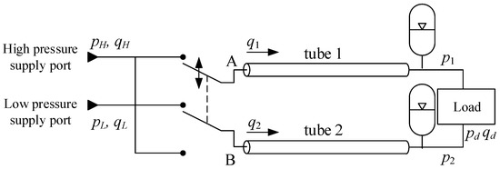
Figure 1.
Schematics of a switched inertance hydraulic system (SIHS) in a four-port valve configuration [3].
The pressure and flow responses in the two tubes with an ideal instantaneous switching transition are shown in Figure 2, where the lumped parameter model is plotted in Figure 2a and the distributed parameter model including the wave propagation effect is shown in Figure 2b. Both types of analytical model will be discussed in the following sections. The high supply pressure is pH and the low supply pressure is pL. p1 is the downstream pressure of the tube 1 and p2 is the load-end pressure of the tube 2, as shown in Figure 1. q1 is the inlet flow rate of the tube 1, q2 is the inlet flow rate of the tube 2, and and are the average flow rates from the HP and LP supply ports. The switching cycle time is T, and the switching ratio is α (a value between 0 and 1, the two extremes meaning the switch in Figure 1 is permanently down or up respectively).
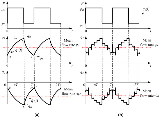
Figure 2.
Supply pressure (pressure for point A in Figure 1) and flow rate with an ideal instantaneous switching transition: (a) lumped parameter model; and (b) distributed parameter model.
Assuming the SIHS operates with 100% efficiency the ideal delivery flow can be given by Equation (1) [2,19]:
where the delivery flow qd is higher than the high pressure port flow.
The ideal delivery pressure can be calculated by using Equation (2) [2,3,19]:
which shows the delivery pressure is proportional to the input pressure difference. From Equations (1) and (2), it can be seen that the zero delivery pressure pd occurs when the switching ratio is 0.5. In this case, the delivery flow rate would be zero as the zero delivery pressure gradient.
In this article, the analytical models of an SIHS in a four-port high-speed switching valve configuration are proposed, and the system dynamics and performance are investigated theoretically and experimentally. The analytical models help to understand the physical characteristics of switched hydraulics and allow the effect of system parameter changes to be investigated. First, a lumped parameter model and a distributed parameter model are developed and the derived equations give a clear relationship between supply pressure, delivery flow rate, flow loss, and power loss of a four-port SIHS. This is followed by experimental validation on a four-port SIHS test rig which employs a high-speed rotary valve as the switching component. Comparisons between the three-port and four-port SIHS and the conventional valve controlled system are presented in terms of power consumption, followed by discussions and conclusions.
2. Lumped Parameter Model
The lumped parameter model simplifies the description of the behaviour of the distributed physical system into a system consisting of discrete entities that approximate the behaviour of the distributed system under certain assumptions. The lumped parameter model consisting of a series of resistors, inductors and capacitors is used for modelling laminar flow in the inertance tube [4,8]. Figure 3 shows the schematic of the lumped parameter model, in which pH and pL are the high and low supply pressures, and pd is the delivery pressure. R is the system resistance (through one valve path and one tube) and I represents the inertance of the tube.
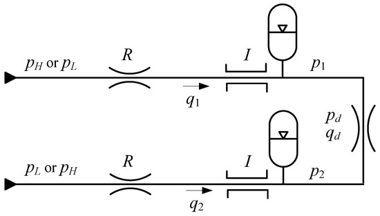
Figure 3.
Lumped parameter model for an SIHS in a four-port switching valve configuration.
The laminar dynamic flow rate q1 and q2 can be calculated using the lumped parameter model, as shown in Equations (3) and (4) [19]:
where α is the switching ratio, T is the switching cycle time, R is the overall system resistance, is the delivery flow rate (assumed constant), and τ is the time constant . The first expression in Equation (3) for increasing q1 is an exponential rise. The flow rate would increase to the steady-state value as shown in Figure 3 if the input pressure remained at pH (no switching) and decrease to if the pressure of entry remained at pL. q2 is in the opposite direction of q1, and qd is the delivery flow rate.
The average flow rate from the HP port corresponds to the sum of the integrals of the expressions in Equation (3) through the one switching period divided by T, given by Equation (5):
Thus:
Definition 1.
The actual average flow rate from the HP supply port is higher than the theoretical flow rate as given by Equation (1) in practice. The flow loss is defined as the difference between the actual and theoretical average flow rate from the HP/LP port.
The laminar flow loss in the time-domain can be described as [19]:
which leads to Theorem 1.
Theorem 1.
The flow loss is affected by the pressure difference between the HP and LP ports, system resistance and inertance and the switching frequency and ratio. It is independent of the delivery flow rate.
3. Distributed Parameter Model
A distributed parameter model assumes that the attributes of the circuit—such as resistance, inductance, and capacitance—are distributed continuously throughout the circuit. This is in contrast to the lumped parameter model [20]. Analytical distributed parameter models of an SIHS in three-port valve configuration have been created and validated in simulation in the authors’ recent work [4,5,6]. For a four-port SIHS, the entry impedance ZE of tube 1 is given by Equation (8) [21]:
where is the pipe characteristic impedance, Rv is the valve resistance and, ξ is the viscous wave correction factor [22]:
where J0, J1 are Bessel functions of the first kind of orders 0 and 1. j is the imaginary unit, r is the internal radius of the tube, ω is radian frequency, and ν is the kinematic viscosity.
The Fourier transform of the supply pressure is:
where n is the number of harmonics.
The Fourier transform of the flow rate is:
Substituting Equations (8)–(11), the Fourier flow rate is:
The flow rate q1 and q2 in the time-domain for a function of period T can be calculated by:
The average flow rate qm from the HP port is:
The distributed flow loss in the time-domain can be described as:
Theorem 2.
The wave propagation has significant effects on the SIHS dynamics. The optimal switching cycle equals to the wave propagation time divided by the switching ratio α or (1 − α):
where is the wave propagation time , c is the speed of sound [5,23].
4. Experimental Validation
4.1. High-Speed Rotary Switching Valve
The dynamics of the switching valve have a substantial effect on the SIHS performance. The valve should be able to operate with a very high switching frequency, a low leakage, and deliver a high flow rate. A high-speed rotary switching valve was designed and used in an SIHS to continuously switch flow between the HP and LP supply ports [6]. There are two supply ports (HP and LP) and two delivery ports (A and B). Steady state tests showed that the valve could deliver 40 L/min flow rate at 10 bar pressure drop [6]. The schematic of the valve is presented in Figure 4a. A brushless servo motor (Baldor BSM50N-375AF, maximum speed 5100 rpm; Baldor: Fort Smith, AR, USA) is used to drive the rotor, and the control shaft adjustment is used to control the switching ratio manually. An angular position controller could be used for the control shaft for automatic switching ratio adjustment. The drive arrangement of the rotary valve is shown in Figure 4b.
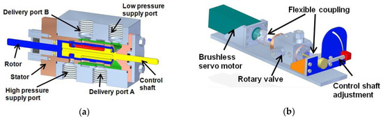
Figure 4.
(a) Schematic of the rotary valve; (b) Arrangement of rotary valve and servo motor, adapted from Pan et al. [6], with permission from © 2015 American Society of Mechanical Engineers, 2015 [6].
Figure 5 shows the flow-pressure characteristics of the valve orifice when it was fully opened. The oil temperature was 54 °C. The estimated orifice opening is 0.238 cm2, assuming the flow coefficient is 0.6 and the fluid density is 860 kg/m3. The valve is modelled by using the standard orifice equation:
where ΔP is the pressure drop across the valve.
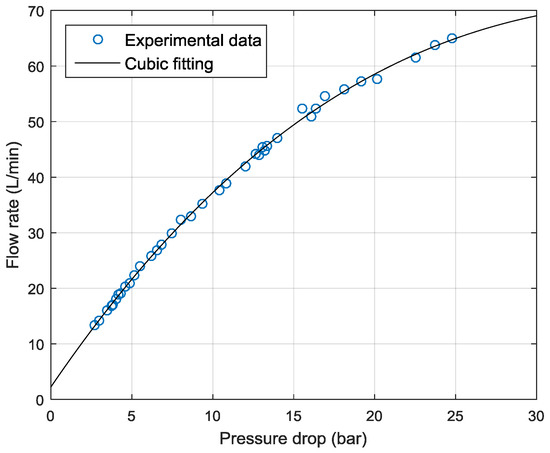
Figure 5.
Valve orifice flow-pressure characteristics.
4.2. Experimental Rig
Figure 6 shows the schematic and photograph of the test rig. The system consists of the high-speed rotary switching valve, two inertance tubes (160 cm each) and a loading system comprising a pressure compensated valve and a needle valve. Three accumulators and in-line shock suppressors were used to attenuate pressure pulsations. Three miniature piezoresistive pressure transducers with a range of 200 bar were used to measure the upstream pressure between the switching valve and the tube, the mid-stream pressure at the connection and the downstream pressure. Two further pressure transducers, with ranges of 350 bar and 35 bar were used to measure the HP and LP supply pressures. There was no pressure transducer at the load end of tube 2 so delivery pressure could not be determined directly. Instead the load-end pressure of the tube 2 is estimated using . An xPC Target real-time platform was used for data acquisition and control, and the numerical models are constructed in SIMULINK. Parameters for the distributed analytical and simulation models are listed in Table 1, which are also used for experiments. Details of simulation models can be found in [19].
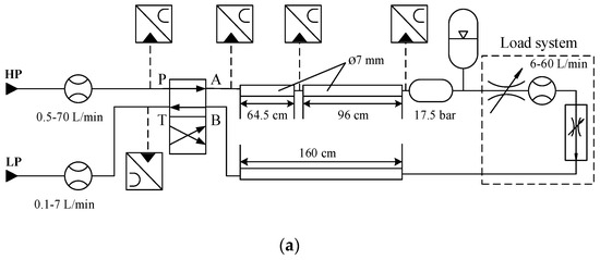
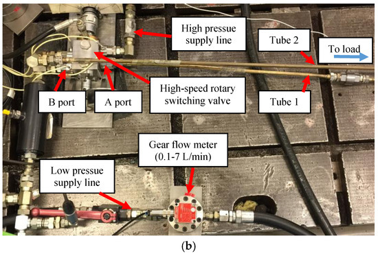
Figure 6.
SIHS test rig in a four-port switching valve configuration (a) Schematic of the rig; (b) Photo of the rig.

Table 1.
Simulation and experimental parameters for an SIHS in a four-port valve configuration.
4.3. Upstream Pressure and Flow Rate at A Port
The HP supply was fixed at 32 bar and the LP at 10 bar. To simplify the system and eliminate the effect of resistance, the needle valve was closed, and the delivery flow rate was 0 L/min. This also helped to reduce the consequences of the valve switching transition and cavitation. The pressure at point A between the switching valve and tube 1 is plotted in Figure 7, where the analytical, simulated, and experimental results agree very well. The electrical noise caused by the sensor measurement was filtered. The pressure switched from 31 bar to 11 bar with the switching ratio of 0.5. The wave propagation effect was almost eliminated with this operating condition (switching ratio = 0.5, switching frequency = 100 Hz). As the optimal operating condition is of the 100 Hz switching frequency and the 0.24 switching ratio (Theorem 2, Equation (17)), some oscillations still can be seen in Figure 7 and Figure 8. The high-frequency resonances have not been fully adapted in this case, which may cause high-frequency noise. However, the oscillations decayed rapidly and did not affect system dynamics and stability. The valve switching transition effect was small due to the zero flow rate. Less clear experimental results are expected when the system operates with a high delivery flow rate. Figure 8 shows the inlet dynamic flow rates. As it was difficult to measure the dynamic flow rate accurately due to the limitation of the sensors, the simulated results were used for comparison in this case. However, we are confident in using the simulated flow rates here as the simulated and experimental pressures agreed very well as shown in Figure 7, which indicates that the simulation is able to represent the system dynamics correctly and accurately.
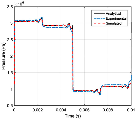
Figure 7.
Analytical and experimental upstream pressures at A port (switching ratio 0.5).
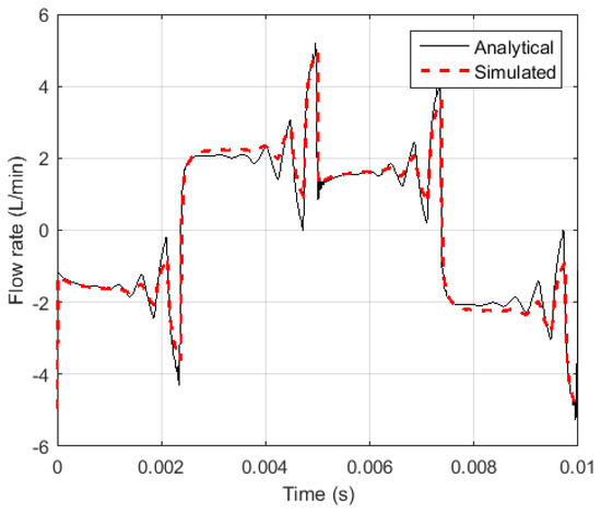
Figure 8.
Analytical and simulated inlet dynamic flow rates for tube 1 (switching ratio 0.5).
The analytical model can effectively predict the dynamic flow rate which gives a novel tool for investigating an SIHS from the fundamental viewpoint without the necessity of creating numerical simulation models requiring a long computation time.
Figure 9 shows the relationship between the delivery pressure and the switching ratio with a switching frequency of 100 Hz. The analytical and experimental results match well and indicate that the delivery pressure has a linear relationship with the switching ratio.
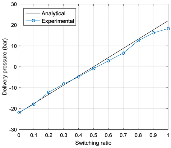
Figure 9.
Analytical and experimental delivery pressures.
Unlike the results from an SIHS in a three-port valve configuration [4], the four-port valve configuration is shown to be able to generate bidirectional pressure difference across the load.
4.4. Flow Loss and System Efficiency
The minimum flow loss occurs when the switching frequency and ratio satisfy Equation (17). Figure 10 shows the analytical and experimental flow loss versus switching ratio with the switching frequency of 100 Hz. Three optimal operating ratios (0.25, 0.5, and 0.75) leading to low flow losses were found, and this was also consistent with Figure 7, where the wave propagation effect was small for a switching ratio of 0.5 [23]. The wave propagation time twave is 2.4 ms.
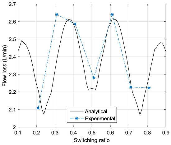
Figure 10.
Analytical and experimental system flow losses.
The input power of the system can be given by Equation (19):
and the system power loss is:
which shows the power loss in a four-port configuration SIHS is influenced by the system flow loss, supply pressure difference, delivery flow rate, and resistance [19].
The system efficiency can be described as:
when the system has an over-running load, the regenerative efficiency is defined as:
Compared with an SIHS in a three-port valve configuration analytically, the four-port valve configuration with the same orifice area consumes more energy (4.5 times) but can drive bidirectionally, as shown in Figure 11. Parameters in Table 1 are used for both configurations, assuming the delivery flow rate was 10 L/min. Compared with a conventional valve controlled system, assuming the required delivery pressure and flow rate were 6 bar and 10 L/min and the supply pressure and flow rate were (32−10) bar and 20 L/min, the system efficiency is 13.6% and the power loss is 633 Watts. With the same working requirements (6 bar at 10 L/min), the estimated switching ratio of the SIHS is 0.84 and the optimal switching frequency is 67.5 Hz. The power loss of the SIHS is 160 Watts and system efficiency is 31%, which is fairly good as the high system resistance 50 bar/(L/s) was applied. This assumption is based on the use of two small diameter inertance tubes, and the fact that the valve will cause extra power loss during the switching transition period. Figure 12 shows the comparison of power losses with a range of delivery pressures and a fixed flow rate 10 L/min. The power loss of the conventional valve controlled system is about six times (on average) that of the four-port valve SISH configuration.
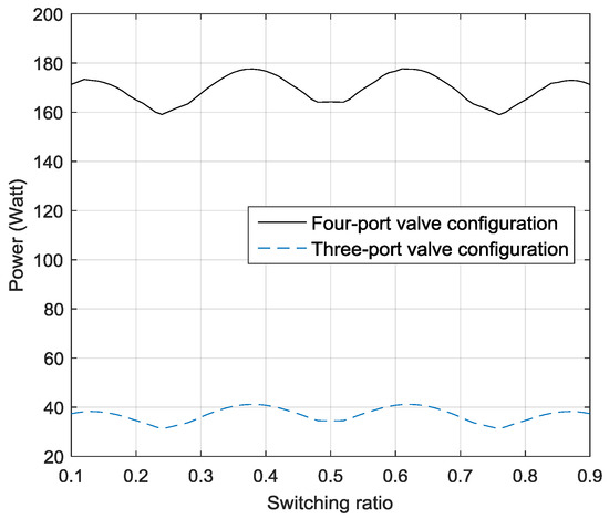
Figure 11.
Comparison of power losses between an SIHS in a three-port valve and a four-port valve configuration.
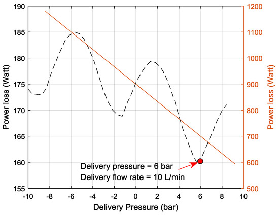
Figure 12.
Comparison of power losses between an SIHS and a conventional valve controlled system.
5. Discussion
The proposed analytical models can predict SIHS dynamics effectively and accurately, as has been validated through comparison with results from both simulation and experiment. Some future work needs to be undertaken. The effects of the system resistance and the delivery flow rate can be investigated in depth with an increased delivery flow rate. This will result in system pressure loss. The HP pressure can be increased with an appropriate delivery flow rate, which will form a more realistic hydraulic circuit for investigation. However, the SIHS test rig operating with a zero flow rate is sufficient for proof of principle of the device, understanding the wave propagation effects and verifying the analytical models.
Assuming the system resistance is a constant R, the pressure loss is expected to have a linear relationship with the delivery flow . In practice, system leakage, the switching transition, and non-linearity of the valve need to be considered, which will result non-linear resistances and performance. The analytical model including these effects is being developed and will be presented in a later article.
6. Conclusions
The analytical model of an SIHS in a four-port switching valve configuration has been shown to be very accurate. The SIHS functions as a conventional four-port valve with the ability to provide bidirectional control of the flow. Two inertance tubes allow continuous inertia in the circuit when the valve switches fast and cyclically. The four-port SIHS can be seen as one three-port flow booster and one three-port pressure booster connecting in series. The analytical models based on a lumped parameter approximation clearly show the relationship of the flow loss, switching frequency, and supply pressures. The distributed parameter models can predict the optimal operating parameters to give the most efficient performance effectively. In addition, the analytical models provide time-efficient solutions directly without running high computation simulation models. The proposed models have been validated experimentally.
The four-port switching valve SIHS is a promising approach for increasing energy efficiency in fluid power systems. Although very duty cycle dependent, the example given in the paper shows power loss reduced to about one-seventh of the loss expected using a conventional throttling valve for control.
Acknowledgments
This work was supported by the UK Engineering and Physical Sciences Research Council under grant number EP/H024190/1 and EP/P022022/1, together with Instron, J.C. Bamford Excavators Limited, and Parker Hannifin.
Author Contributions
Min Pan developed the models, conceived and designed the experiments, analysed the data and wrote the paper; Andrew Plummer made valuable suggestions and contributed to the manuscript editing; Abdullah El Agha assisted with the experiments and instrumentation work.
Conflicts of Interest
The authors declare no conflict of interest.
References
- Brown, F.T. Switched reactance hydraulics: A new way to control fluid power. In Proceedings of the National Conference on Fluid Power, Chicago, IL, USA, 2–5 March 1987; pp. 25–34. [Google Scholar]
- Brown, F.T. A hydraulic rotary switched inertance servo-transformer. J. Dyn. Syst. Meas. Control 1988, 110, 144–150. [Google Scholar] [CrossRef]
- Johnston, D.N. A switched inertance device for efficient control of pressure and flow. In Proceedings of the Bath/ASME Fluid Power and Motion Control Symposium, Hollywood, CA, USA, 12–14 October 2009. [Google Scholar]
- Pan, M.; Johnston, D.N.; Plummer, A.; Kudzma, S.; Hillis, A. Theoretical and experimental studies of a switched inertance hydraulic system. Proc. Inst. Mech. Eng. Part I J. Syst. Control Eng. 2014, 228, 12–25. [Google Scholar] [CrossRef]
- Pan, M.; Johnston, D.N.; Plummer, A.; Kudzma, S.; Hillis, A. Theoretical and experimental studies of a switched inertance hydraulic system including switching transition dynamics, non-linearity and leakage. Proc. Inst. Mech. Eng. Part I J. Syst. Control Eng. 2014, 228, 802–815. [Google Scholar] [CrossRef]
- Pan, M.; Johnston, D.N.; Robertson, J.; Plummer, A.; Hillis, A.; Yang, H. Experimental investigation of a switched inertance hydraulic system with a high-speed rotary valve. Trans. ASME J. Dyn. Syst. Meas. Control 2015, 137, 121003. [Google Scholar] [CrossRef]
- Kogler, H.; Scheidl, R. Energy efficient linear drive axis using a hydraulic switching converter. J. Dyn. Syst. Meas. Control 2016, 138, 091010. [Google Scholar] [CrossRef]
- Scheidl, R.; Manhartsgruber, B.; Kogler, H.; Winkler, B.; Mairhofer, M. The hydraulic buck converter–concept and experimental results. In Proceedings of the Sixth International Conference on Fluid Power, Dresden, Germany, 31 March–2 April 2008. [Google Scholar]
- Kogler, H.; Scheidl, R. Two basic concepts of hydraulic switching converters. In Proceedings of the First Workshop on Digital Fluid Power, Tampere, Finland, 3 October 2008. [Google Scholar]
- Kogler, H.; Scheidl, R. The hydraulic buck converter exploiting the load capacitance. In Proceedings of the 8th International Fluid Power Conference (8. IFK), Dresden, Germany, 26–28 March 2012; Volume 2, pp. 297–309. [Google Scholar]
- Kogler, H.; Scheidl, R.; Ehrentraut, M.; Guglielmino, E.; Semini, C.; Caldwell, D.G. A Compact Hydraulic Switching Converter for Robotic Applications; Fluid Power and Motion Control: Bath, UK, 2010; pp. 55–66. [Google Scholar]
- Scheidl, R.; Garstenauer, M.; Manhartsgruber, B. Switching Type Control of Hydraulic Drives—A Promising Perspective for Advanced Actuation in Agricultural Machinery; SAE Technical Paper No. 2000-01-2559; SAE International: Warrendale, PA, USA, 2009. [Google Scholar]
- Scheidl, R.; Manhartsgruber, B.; Kogler, H. Mixed time-frequency domain simulation of a hydraulic inductance pipe with a check valve. Proc. Inst. Mech. Eng. Part C 2011, 225, 2413–2421. [Google Scholar] [CrossRef]
- Wang, F.; Gu, L.; Chen, Y. A continuously variable hydraulic pressure converter based on high-speed on–off valves. Mechatronics 2011, 21, 1298–1308. [Google Scholar] [CrossRef]
- Van de Ven, J.D. On fluid compressibility in switch-mode hydraulic circuits—Part I: Modeling and analysis. ASME J. Dyn. Syst. Meas. Control 2013, 135, 021013. [Google Scholar] [CrossRef]
- Rannow, M.B.; Li, P.Y. Soft switching approach to reducing transition losses in an on/off hydraulic valve. J. Dyn. Syst. Meas. Control 2012, 134, 064501. [Google Scholar] [CrossRef]
- Pan, M.; Johnston, N.; Hillis, A. Active control of pressure pulsation in a switched inertance hydraulic system. Proc. Inst. Mech. Eng. Part I Syst. Control Eng. 2013, 227, 610–620. [Google Scholar] [CrossRef]
- Pan, M. Adaptive control of a piezoelectric valve for fluid-borne noise reduction in a hydraulic buck converter. Trans. ASME J. Dyn. Syst. Meas. Control 2017, 139. [Google Scholar] [CrossRef]
- Johnston, D.N.; Pan, M.; Plummer, A.; Hillis, A.; Yang, H. Theoretical studies of a switched inertance hydraulic system in a four-port valve configuration. In Proceedings of the Seventh Workshop on Digital Fluid Power, Linz, Austria, 26–27 February 2015. [Google Scholar]
- Akers, A.; Gassman, M.; Smith, R. Hydraulic Power System Analysis; CRC Press: Boca Raton, FL, USA, 2006. [Google Scholar]
- Johnston, D.N. Measurement and Prediction of the Fluid Borne Noise Characteristics of Hydraulic Components and Systems. Ph.D. Thesis, University of Bath, Bath, UK, 1987. [Google Scholar]
- Stecki, J.S.; Davis, D. Fluid transmission lines—Distributed parameter models Part 1: A review of the state of the art. Proc. Inst. Mech. Eng. Part A J. Power Energy 1986, 200, 215–228. [Google Scholar] [CrossRef]
- Wang, P.; Kudzma, S.; Johnston, D.N.; Plummer, A.; Hillis, A.J. The influence of wave effects on digital switching valve performance. In Proceedings of the Fourth Workshop on Digital Fluid Power, Linz, Austria, 21–22 September 2011. [Google Scholar]
© 2017 by the authors. Licensee MDPI, Basel, Switzerland. This article is an open access article distributed under the terms and conditions of the Creative Commons Attribution (CC BY) license (http://creativecommons.org/licenses/by/4.0/).